Wildfire Identification Based on an Improved Two-Channel Convolutional Neural Network

Abstract

The identification of wildfires is a very complex task due to their different shapes, textures, and colours. Traditional image processing methods need to manually design feature extraction algorithms based on prior knowledge, and because fires at different stages have different characteristics, manually designed feature extraction algorithms often have insufficient generalization capabilities. A convolutional neural network (CNN) can automatically extract the deeper features of an image, avoiding the complexity and blindness of the feature extraction phase. Therefore, a wildfire identification method based on an improved two-channel CNN is proposed in this paper. Firstly, in order to solve the problem of the insufficient dataset, the dataset is processed by using PCA_Jittering, transfer learning is used to train the model and then the accuracy of the model is improved by using segmented training. Secondly, in order to achieve the effective coverage of the model for fire scenes of different sizes, a two-channel CNN based on feature fusion is designed, in which the fully connected layers are replaced by a support vector machine (SVM). Finally, in order to reduce the delay time of the model, Lasso_SVM is designed to replace the SVM in the original model. The results show that the method has the advantages of high accuracy and low latency. The accuracy of wildfire identification is 98.47% and the average delay time of fire identification is 0.051 s/frame. The wildfire identification method designed in this paper improves the accuracy of identifying wildfires and reduces the delay time in identifying them.

1. Introduction

As the Earth’s climate changes, wildfires occur frequently around the world, causing serious economic losses and ecological damage [1]. In 2019–2020, more than 24 million hectares of land in south-eastern Australia were burned by wildfires, resulting in 33 deaths and more than 3000 houses being razed. A total of 80% of the Australian population was affected by the smoke from the wildfire, which killed 445 people, hospitalised more than 4000 and cost $2 billion in medical treatment. The wildfires caused billions of dollars of damage, emitted 400–700 million tonnes of carbon, and killed 3 billion wild animals [2]. Fire affects the biodiversity, species composition, and ecosystem structure of forest ecosystems, in addition to human livelihoods, regional economies, and environmental health [3]. Intelligent monitoring of wildfire is therefore of great importance.

Image-based fire identification has become a research focus in recent years. There are two main types of image-based wildfire identification methods: one is a traditional image processing method and the other is the identification method based on CNN [4].

Traditional image processing methods have been used to identify fires by extracting features such as colour, geometry and dynamic texture. Kong et al. [5] proposed a fire identification method based on temporal smoothing and logistic regression, which used background subtraction to obtain colour component ratios and running cues of fires to identify suspected fire regions and used logistic regression to identify fires based on the size, motion and colour characteristics. Mei et al. [6] proposed a new method for fire identification which first extracted suspected fire regions by random forest, support vector machine and improved ViBe algorithms, and then used fire overlap rate and motion intensity rate between each frame and Hu features to identify fires. Dimitropoulos et al. [7] fused the features of fire smoke according to a dynamic fractional union approach and then classified them by SVM to finally identify fire smoke. Gong et al. [8] proposed a fire identification method based on multiple features of fires, which extracted suspected fire regions by identifying the motion and colour of the images and calculated the fire centre of mass for each frame to identify fires by extracting the spatial, shape, and area variability of the images. Prema et al. [9] proposed a multi-feature-based fire smoke identification method, which extracted suspected fire smoke regions by filtering in the YUV colour space and extracted the spatio-temporal features of the regions to identify fire smoke by SVM. Han et al. [10] used a fire identification method based on a Gaussian mixture model and multicolor features to extract moving objects from the video, then combined RGB, HSI and YUV color spaces to extract suspected fire regions and combined the results obtained above to identify fires. Chu et al. [11] proposed a probabilistic inference framework to determine fire location and fire size, and to estimate multidimensional fire parameters using Bayesian inference theory.

However, traditional image processing methods rely on prior knowledge to determine the feature extraction algorithms for fires, and the morphology of fires can produce different features at different stages, making it difficult for the same fire feature extraction algorithm to cater for different fire scenarios, and therefore their generalization capability is weak. The deep fire features can be found automatically by CNN-based image identifying methods [12], which avoids the limitations caused by the selection of image features by subjective human factors, thus greatly improving the accuracy of identifying. Zhang et al. [13] proposed a two-layer CNN-based method for wildfire identification, which first used a CNN with a larger input resolution to detect the image and then used a fine-grained CNN to pinpoint the fire if a wildfire was detected. Kim et al. [14] used Faster-RCNN to detect suspected fire regions and non-fire regions based on spatial features and detect the presence of fire in the short term by accumulating summary features within bounding boxes in successive frames using Long Short-Term Memory (LSTM), and then successive short-term results were combined into a majority vote to make the final decision. Zhang et al. [15] proposed an effective SqueezeNet-based asymmetric encoder-decoder U-shape architecture ATT Squeeze U-Net to identify wildfire. Muhammad et al. [16] proposed a computationally efficient CNN model based on the Squeezenet architecture, which used smaller convolutional kernels and removed the fully connected layers to achieve high computational efficiency. Han et al. [17] proposed an effective method for wildfire identification, which combined CNN and RNN to enable the model to process sequential data, and the method achieved good identification results in various fire scenarios. Wu et al. [18] used a deep learning-based method for the identification of fire and smoke which used ViBe and frame difference methods to extract regions of motion and used features extracted using Alexnet and the degree of irregularity of fire and smoke as static features, combining dynamic and static features to eventually identify regions of fire and smoke.

The comparisons between extracting wildfire features with traditional image processing methods and deep learning methods are shown in

Table 1. The comparisons between two wildfire feature extraction methods.

Methods	Comparisons
Traditional methods	Rely on manual extraction of features, which is highly subjective;
	Rely on priori knowledges to extract features;
	The extracted features are relatively simple;
	The method has a low generalization capability.
Deep learning methods	Features can be extracted automatically with low subjectivity;
	Feature extraction without reliance on prior knowledge;
	Deep features can be extracted;
	The method has a strong generalization capability.

.

Despite its accomplishments in wildfire identification, CNN suffers from significant latency. Reducing the delay time by lightening the network structure of the CNN leads to a reduction in model accuracy. In order to solve the problems above, a wildfire identification method based on an improved two-channel CNN is proposed, aiming to achieve high accuracy and low latency of the model. In this method, first, the dataset is expanded with an image enhancement strategy, training is performed using transfer learning, and model accuracy is improved using segmented training. Next, a two-channel CNN is designed, and feature fusion of the two-channel CNN is implemented. Finally, the structure of the two-channel CNN is modified to reduce the delay time of the model in identifying images. The results of the study may provide useful information for the improvement of wildfire identification algorithms.

2. Construction of the Experimental Dataset

The dataset used in this paper is obtained from the Google search engine and contains three main parts. Part one includes wildfire scenes, which contains images of large fires and smoke, as shown in Figure 1. There are no special restrictions on the place of wildfires, and they are available at various times of the day. Part two includes regular forest scenes, which contain images of the forests without fires and smoke, as shown in Figure 2. As the identifying of wildfire is susceptible to sunlight, part three includes sun scenes, which contain sunset images and sunset images when there are large areas of clouds, as shown in Figure 3. There are 14,000 images in the dataset. A total of 10,000 images are selected as the training set and 4000 images as the testing set, with 5000 fire and 5000 non-fire images in the training set and 2000 fire and 2000 non-fire images in the testing set.

The accuracy of the model is strongly influenced by the dataset. When the size of the dataset is minimal, the model is prone to overfitting, resulting in the model’s accuracy for the training set being substantially larger than the model’s accuracy for the testing set. In order to reduce the overfitting of the model and improve its generalization ability, the PCA_Jittering image enhancement [19] strategy is adopted in this paper, thus expanding the training set. Firstly, principal component analysis (PCA) is used on the three RGB channels of the training set to obtain the covariance matrix and calculate the eigenvalues and eigenvectors. Next, Gaussian jitterings are added to the eigenvalues and the eigenvalues are multiplied by the eigenvectors. Finally, the multiplication results are added to the original image, modifying the intensity of the image’s three RGB channels, and the image using PCA_Jittering image enhancement is added to the training set for training. The flowchart of PCA_Jittering is shown in Figure 4.

The specific steps of PCA_Jittering are as follows:

(1).

Obtain the original image $I_{\mathrm{x}y}$ of the wildfire, split the three RGB channels of the original image $I_{\mathrm{x}y}$, and obtain the values $I_{xy}^R, I_{xy}^G, I_{xy}^B$ of the three channels.

(2).

Using $I_{xy}^R$ as an example, $I_{xy}^R$ are normalised to eliminate the effect of odd data. The normalisation formula is shown in Equation (1).

$$I_{xy}^R=\frac{I_{xy}^R}{255.0}$$

(1)

(3).

To unify the scale of the images, $I_{xy}^R$ are standardised. The standardisation formula is shown in Equation (2).

$$g_{ij}^R=\frac{x_{ij}^R-{\mu }^R}{{\sigma }^R}$$

(2)

where $x_{ij}^R$ denotes the grayscale value of row i and column j of the R-channel image of wildfire; $g_{ij}^R$ denotes the standardised grayscale value of row i and column j of the R-channel image of wildfire; ${\mu }^R$ denotes the arithmetic mean of the R-channel, ${\mu }^R=\frac{1}{n\times m}{\displaystyle \sum _{i=1}^n{\displaystyle \sum _{j=1}^m{x}_{ij}^R}}$, n denotes the number of rows of the image and m denotes the number of columns of the image; ${\sigma }^R$ denotes the standard deviation of the R-channel, ${\sigma }^R=\sqrt{\frac{1}{n-1}{{\displaystyle \sum _{i=1}^n(x_{ij}^R-{\mu }^R)}}^2}$.

(4).

Expand the standardised $g_{ij}^R$ into a column of vector $g^R={[g_1^R g_2^R \dots g_{m\times n}^R]}^{\mathrm{T}}$.

(5).

$I_{xy}^G$ and $I_{xy}^B$ are processed in the same way as $I_{xy}^R$. After processing, the standardised vectors $g^G$ and $g^B$ for the G and B channels are obtained, and $g^R, g^G, g^B$ vectors are formed into a matrix T.

$$T=\left[\begin{array}{ccc}{g}_1^R& g_1^G& g_1^B\\ g_2^R& g_2^G& g_2^B\\ ⋮& ⋮& ⋮\\ g_{m\times n}^R& g_{m\times n}^G& g_{m\times n}^B\end{array}\right]=\left[{\mathrm{g}}^R{ \mathrm{g}}^G{ \mathrm{g}}^B\right]$$

(3)

(6).

Create a covariance matrix S of T. The formula for the covariance matrix S is shown in Equation (4).

$$S=\left[\begin{array}{ccc}cov(g^R,g^R)& cov(g^R,g^G)& cov(g^R,g^B)\\ cov(g^G,g^R)& cov(g^G,g^G)& cov(g^G,g^B)\\ cov(g^B,g^R)& cov(g^B,g^G)& cov(g^B,g^B)\end{array}\right]$$

(4)

where $cov(g^w,g^v)=\frac{1}{n-1}{\displaystyle \sum _{i=1}^{m\times n}(g_i^w-\overline{g^w})(g_i^v-\overline{g^v})}$, $w,v\in [R,G,B]$, $\overline{g^w}$ and $\overline{g^v}$ denote the average of the w and v columns, respectively.

(7).

Solve for the eigenvectors $p_i$ and eigenvalues ${\lambda }_i$ of the covariance matrix S, where $i\in [1,2,3]$.

(8).

Multiply the eigenvalues ${\lambda }_i$ by Gaussian jitterings ${\alpha }_i$ with 0 as the mean and 0.1 as the variance, then multiply the eigenvalues after adding jitterings with the eigenvectors and multiply the results by 255 and add them to the original pixel values $I_{\mathrm{x}y}=[I_{xy}^R,I_{xy}^G,I_{xy}^B]$. The pixel values of the image after using PCA_Jittering image enhancement are shown in Equation (5).

$$I_{xy}^{\prime }=[I_{xy}^R,I_{xy}^G,I_{xy}^B]+255\times [p_1,p_2,p_3][{\alpha }_1{\lambda }_1,{\alpha }_2{\lambda }_2,{\alpha }_3{\lambda }_3]$$

(5)

The dominant colours in the RGB channels of the image can be found by PCA_Jittering image enhancement, so that the values of the dominant colours are drastically altered while the overall tone of the image remains unchanged. The images using PCA_Jittering image enhancement are added to the training set. Finally, the wildfire image dataset has a total of 24,000 images, with 20,000 images in the training set and 4000 images in the testing set. There are 10,000 images for each of the fire and non-fire samples in the training set and 2000 images for each of the fire and non-fire samples in the testing set. The comparisons of images before and after using PCA_Jittering image enhancement are shown in Figure 5.

3. Establishment of the Wildfire Identification Model

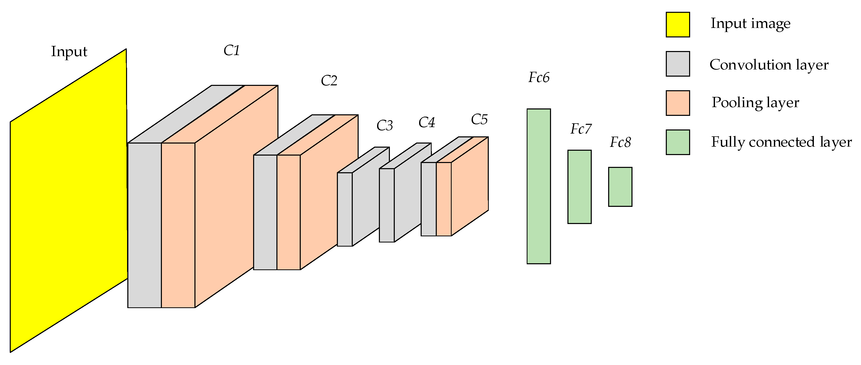
3.1. Modeling of the Alexnet Network

Deep features of fires need to be extracted by CNN. To identify wildfire, Alexnet [19] was used as a CNN architecture in this paper. Alexnet consists of five convolution layers, three pooling layers and three fully connected layers Fc6–Fc8. The convolution and pooling layers form C1–C5. The structure of Alexnet is shown in Figure 6.

Partial features of the image are learned through the convolution kernel of the convolution layer to generate the feature map. The convolution operation is used to extract the different features of the input. The formula for extracting image features from the convolution layer is shown in Equation (6).

$$X_j^l=f({\displaystyle {\sum }_{i\in M_j}{X}_i^l}\times k_{ij}^l+b_j^l)$$

(6)

where $X_j^l$ represents the jth feature map extracted from the lth convolution layer, $f(\cdot )$ represents the activation function, M_j represents the feature map, $k_{ij}^l$ represents the convolution kernel, and $b_j^l$ represents the offset.

Once the image features have been extracted by the convolution kernel, activation functions need to be introduced to allow the model to address non-linear issues. The ReLU activation function can address not only the non-linearity problem of the model, but also the gradient disappearance problem when the network layers are deep, and its expression is shown in Equation (7). Since Leaky ReLU does not always work better than ReLU [20], ReLU is chosen as the activation function in this paper, and the convolution layer is calculated as shown in Equation (8).

$$\mathrm{ReLU}(x)=\max (0,x)$$

(7)

$$X_j^l=\mathrm{ReLU}({\displaystyle {\sum }_{i\in M_j}{X}_i^l}\times k_{ij}^l+b_j^l)$$

(8)

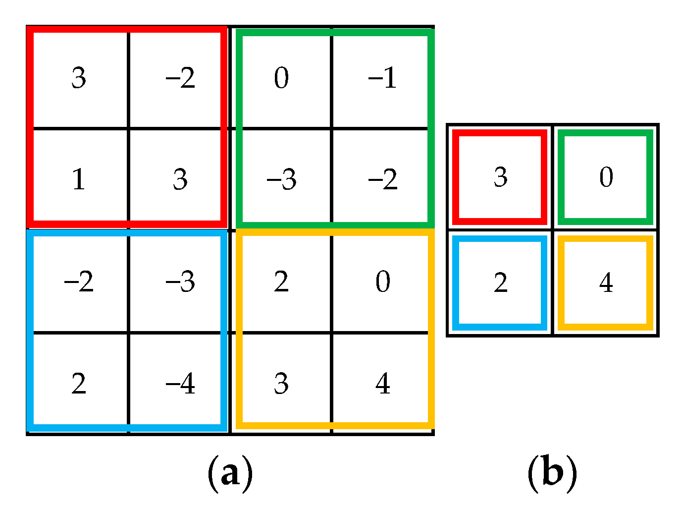
The feature maps obtained from the convolution operation are relatively large, and if they are fed directly into the fully connected layers, the performance of the network will be reduced, while the pooling layer can compress the features extracted from the convolution layer. In this paper, the maximum pooling layer is used to extract features from the convolution layer. Only the largest feature value within the region is retained by the maximum pooling layer, and all other features are ignored by the maximum pooling layer. This not only allows the features to be compressed, but also alleviates the sensitivity of the convolution layer to position, and the effect of noise is reduced. The effect of the maximum pooling layer is shown in Figure 7.

After convolution pooling layers C1–C5, the deep features of wildfire were extracted by CNN. In order to identify fires, deep features are fed into the fully connected layers. The fully connected layers are neural networks with multiple hidden layers that identify wildfire by updating the parameters with a back propagation algorithm.

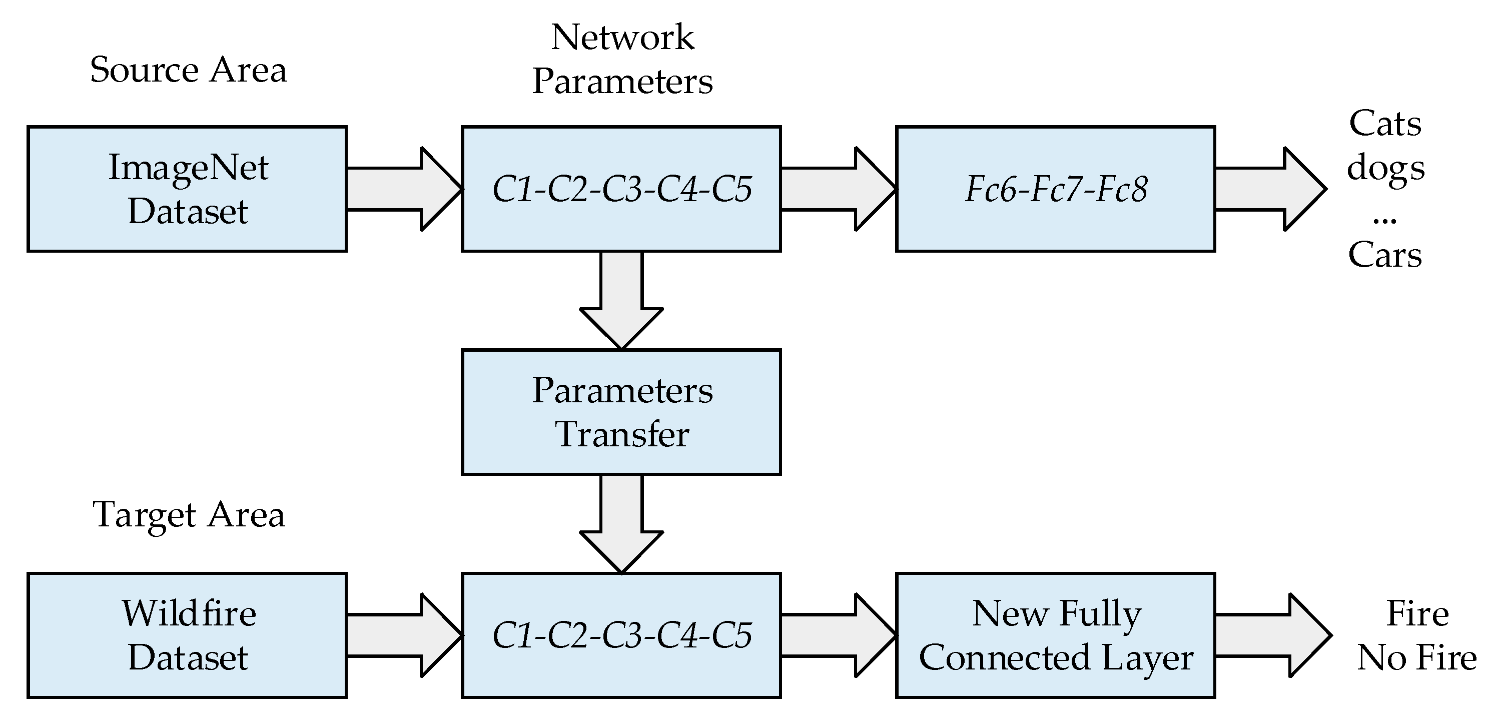
Due to the long training time of Alexnet and the tendency of the model to overfit, transfer learning is used in this paper to train the model. Transfer learning is a machine learning method that reduces the training time and overfitting of a model by transferring parameters from the source domain to the target domain. With transfer learning, the model no longer needs to be trained from a blank CNN. In this paper, the network parameters C1–C5 trained on the large dataset ImageNet are transferred to the target model, the model parameters are initialised, the fully connected layers Fc6_new–Fc8_new for the new task are designed to replace the fully connected layers Fc6–Fc8 in the original model, and finally the network parameters are fine-tuned using the wildfire image dataset. The transfer process in this paper is shown in Figure 8.

In this paper, the number of input neurons of the new fully connected layers is designed to be the number of dimensions of the wildfire features extracted by the convolution pooling layers C1–C5. Since the output of the fully connected layers has two states, fire and no fire, the number of output neurons of the new fully connected layers is designed to be two. The features extracted from the convolution pooling layers C1–C5 are used as inputs to the new fully connected layers. The features extracted by C1–C5 are first fed to the Dropout layer, which can randomly ignore some neurons in the model, and overfitting of the model can be well avoided. Next, the features are dimensionally reduced through Fc6_new. The features are then reduced to two dimensions through the ReLU activation function, Dropout layer, Fc7_new, ReLU activation function and Fc8_new, thus giving the model the ability to identify wildfire. Finally, the features are fed to the softmax layer to output the classification result, which is calculated as shown in Equation (9). The diagram of the new fully connected layers is shown in Figure 9.

$$S_q=\frac{e^q}{{\displaystyle \sum _{w=1}^2{e}^w}}$$

(9)

where q denotes the qth component in the output vector, S_q denotes the classification probability of the qth component, and w denotes the sequence number of the component.

The network settings for the new model are shown in

Table 2. Network settings for the new model.

Type	Input Size	Kernel Size	Kernel Num	Output Size	Stride	Padding
Conv1	227 × 227 × 3	11 × 11	64	56 × 56 × 64	4	2
Pool1	56 × 56 × 64	3 × 3	none	27 × 27 × 64	2	0
Conv2	27 × 27 × 64	5 × 5	192	27 × 27 × 192	1	2
Pool2	27 × 27 × 192	3 × 3	none	13 × 13 × 192	2	0
Conv3	13 × 13 × 192	3 × 3	384	13 × 13 × 384	1	1
Conv4	13 × 13 × 384	3 × 3	256	13 × 13 × 256	1	1
Conv5	13 × 13 × 256	3 × 3	256	13 × 13 × 256	1	1
Pool3	13 × 13 × 256	3 × 3	none	6 × 6 × 256	2	0
Fc6_new	9216	none	none	4096	none	none
Fc7_new	4096	none	none	4096	none	none
Fc8_new	4096	none	none	2	none	none

.

The Adam optimiser is employed in this paper so as to update the model parameters of the CNN. Adam is an adaptive learning rate method with the following equations.

$$m_t = {\beta }_1{m}_{t-1} + (1-{\beta }_1)g_t$$

(10)

$$v_t = {\beta }_2{v}_{t-1} + (1 - {\beta }_2)g_t^2$$

(11)

$${\theta }_{t+1} = {\theta }_t - \frac{\alpha }{\sqrt{{\hat{v}}_t+\epsilon }}\widehat{m_t}$$

(12)

where m_t and v_t are the vectors initialized to zero in the first and second moment estimates of the gradient, respectively, ${\theta }_t$ is the learnable parameter, $\epsilon$ is the smoothing term, $a$ is the adaptive learning rate, and $g_t$ is the gradient distribution.

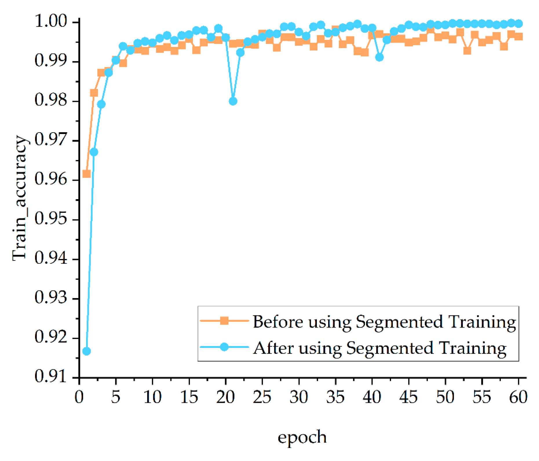
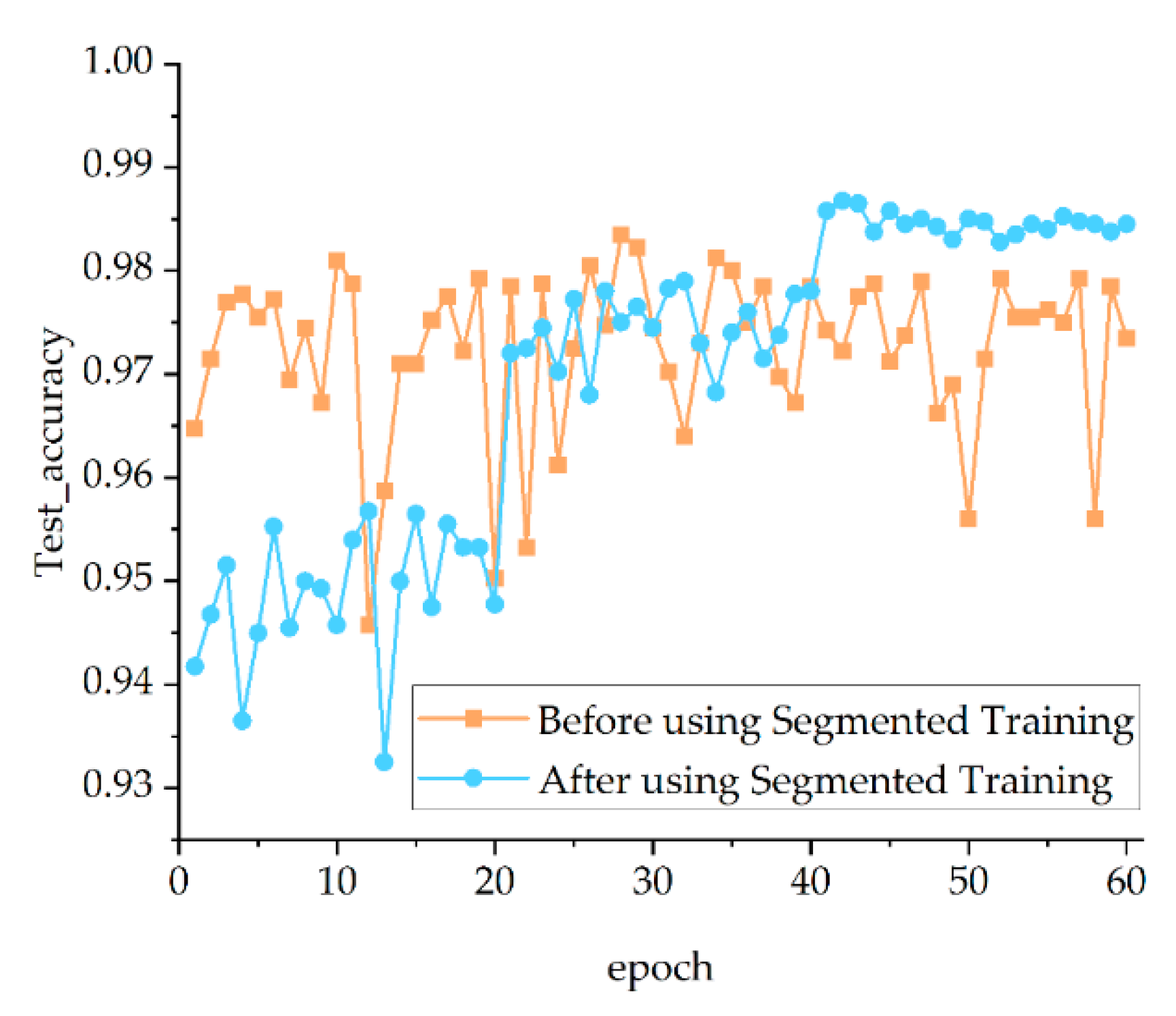
Based on transfer learning, segmented training is used in this paper to further reduce the overfitting of the model. Segmented training means that the image dataset is first set to a low resolution by the model and the model starts training using low resolution images. As the training progresses, the resolution of the dataset is gradually increased and the model parameters from the low resolution are transferred to the new model for training until the resolution reaches the specified size. When training with low resolution images, the overall structure of images is learned by the model, and this information can be refined as the resolution of images is extended.

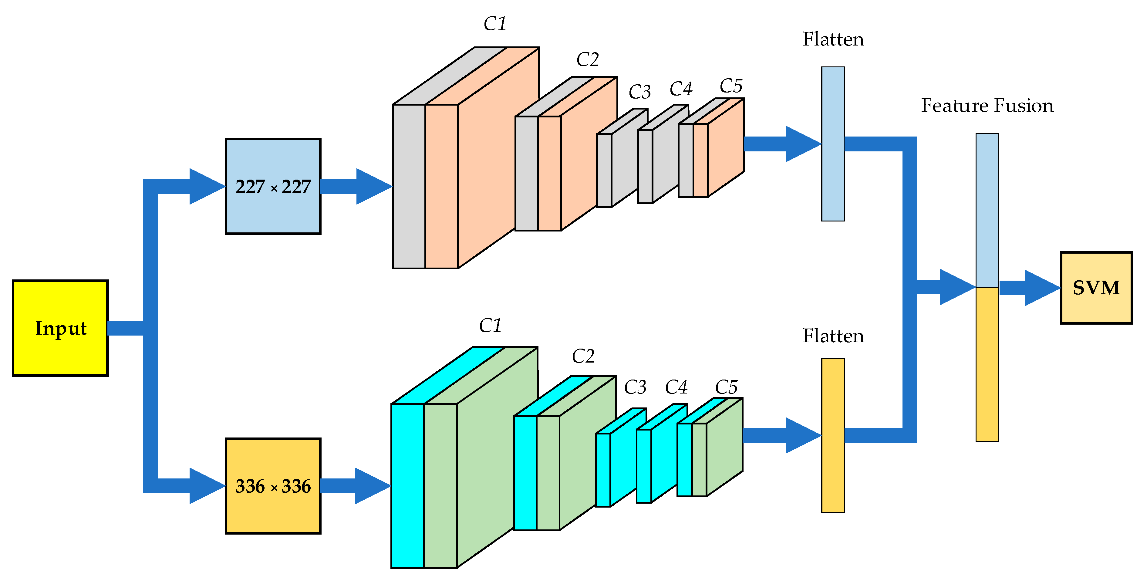
3.2. Development of a Two-Channel CNN

In order to achieve effective coverage of the model for fire scenes of different sizes and thus improve the accuracy of the model, a two-channel CNN based on different resolutions is proposed in this paper. The two-channel CNN has two convolution pooling layer channels, and the inputs of the two channels are wildfire datasets with different resolutions. The resolution of the dataset for the first channel is 227 × 227 and the resolution of the dataset for the second channel is 336 × 336. The convolution pooling layers C1–C5 of both channels are trained simultaneously and wildfire features are extracted independently, and the features are flattened after extraction and fused in a 1:1 ratio. Considering the unique advantages of SVM in small samples and non-linear classification problems, the fully connected layers in the original model are replaced using SVM. The structure of the two-channel CNN is shown in Figure 10.

SVM [21] is a machine learning algorithm that requires less training data and has high model accuracy. The features extracted and fused by the two-channel CNN are trained by SVM to find the optimal segmentation hyperplane of the model and to achieve fire classification. When given an image (x_i,y_i), $y_i\in \left\{-1,1\right\}$ of wildfire, SVM is optimised in the form shown in Equation (13).

$$\begin{array}{c}\underset{w^{i,j},b^{i,j},{\xi }_t^{i,j}}{\min }\frac{1}{2}{\parallel w^{i,j}\parallel }^2 + C{\displaystyle \sum _{t=1}}{\xi }_t^{i,j}\\ s.t {\left(w^{i,j}\right)}^T\varphi \left(x_t\right)+b^{i,j}\ge 1-{\xi }_t^{i,j}, if y_t = i;\\ {\left(w^{i,j}\right)}^T\varphi \left(x_t\right)+b^{i,j}\ge 1-{\xi }_t^{i,j}, if y_t = j;\\ {\xi }_t^{i,j}\ge 0,i<j\end{array}$$

(13)

where w is the normal vector perpendicular to the resulting hyperplane, $\varphi$ is the non-linear mapping, $\xi$ is the relaxation variable, and C is the penalty factor.

After introducing the Lagrange function L = (w,b,a) and implementing the dualisation, the decision function becomes:

$$f_{i,j}(t)=sign({\displaystyle \sum _{l=1}^{n_{sv}^{i,j}}{a}_l^{i,j}}{y}_l^{i,j}k(t,x_l^{i,j})+b^{i,j})$$

(14)

where t is the sample to be classified, n is the number of support vectors, x_i is the fused feature vector, y_i is the corresponding category, $sign(\cdot )$ is the symbolic function, ${\alpha }_i$ is the Lagrangian factor, $k(x,x_i)$ is the kernel function, and b is the classification threshold determined from the training set.

The SVM kernel function used in this paper is a Gaussian radial basis function. The advantages of few parameters and fast convergence are possessed by the Gaussian radial basis function, whose formula is shown in Equation (15).

$$k(t,x_l^{i,j})=\exp (-\frac{{\Vert t-x_i\Vert }^2}{2{\sigma }^2})$$

(15)

where $\sigma$ is the argument to the kernel function.

3.3. Construction of an Improved Two-Channel CNN

Due to the large number of features extracted by the two-channel CNN, feeding them directly to the SVM will result in a large delay time. To address this problem, an improved two-channel CNN is proposed in this paper, which compresses the flattened features from the two channels separately. After feature compression, the improved two-channel CNN performs feature fusion and finally classifies the dataset by SVM.

In this paper, since the features after flattening are high-dimensional sparse data, and linear models have better performance in dealing with these data while being widely used in classification problems [22], Lasso is chosen to compress the features in this paper.

Lasso is a compressed estimate in which some of the eigencoefficients in the model are made to be exactly zero by adding the L₁ parametrization to the model, that is, certain features are completely ignored by the model, thus presenting the most important features of the model and achieving the effect of subset shrinkage [23]. Calculation time can be reduced by reducing the number of dimensions of the original data [24].

Taking one of the two channels in the improved two-channel CNN as an example, the features extracted by the convolution pooling layers C1–C5 are flattened and used as inputs to Lasso, and the output is predicted using Equation (16).

$$\widehat{y}=w_1{x}_1+w_2{x}_2+\dots +w_i{x}_i+b$$

(16)

where x_i denotes the features after flattening, w_i denotes the parameters of the features in the model, b is the offset, and $\widehat{y}$ is the predicted output.

Lasso calculates the loss function $J(w,b)$ from the squared error of the true value y and the predicted value $\widehat{y}$, and adds a regular term to the loss function. Lasso’s loss function is shown in Equation (17).

$$J(w,b)=\frac{1}{2m}{\displaystyle \sum _{i=1}^m{(\widehat{y}-y)}^2+\lambda \cdot \Vert \mathrm{w}\Vert { }_1}$$

(17)

where m is the number of wildfire dataset, n is the number of features after flattening, $\lambda$ is the regularisation parameter, and ${\Vert w\Vert }_{ 1}={\displaystyle \sum _{p=1}^n\left|w_p\right|}$ is the L₁ parametrization.

The objective of Lasso is to achieve variables selection and model parameter estimation, and Lasso’s solution formula is shown in Equation (18).

$$\underset{w\in R^P}{\arg \min }\frac{1}{2m}{\displaystyle \sum _{i=1}^m{(\widehat{y}-y)}^2+\lambda \cdot \Vert \mathrm{w}\Vert { }_1}$$

(18)

4. Experimental Results

This experiment was performed under the Pytorch framework of Windows 10 system, Intel(R) Core (TM) i5-6300HQ 2.3 GHz; 16 GB DDR4 memory; the GPU uses the NVIDIA GTX 950 as the hardware accelerator for model training.

4.1. Simulation Analysis of PCA_Jittering Image Enhancement

PCA_Jittering is used in this paper to achieve image enhancement of the training set by drastically changing the values of the major colour families in the RGB image so that the overall hue of the image does not change. The enhanced images are added to the training set, thus increasing the number of images in the training set. Because of the inconsistent image sizes in the wildfire dataset, the images are first stretched and compressed to a uniform size of 227 × 227 and then the images are standardised. Next, the batch training method is used in this paper and the value of batch_size is set to 8.

The back propagation algorithm is employed by CNN so that the parameters can be updated. The learning rate has a large impact on the back propagation algorithm and the performance of the network is directly determined by the value of the learning rate. Therefore, different learning rates are set in this paper so as to test the effect of learning rate on network performance. The initial learning rate is first set to 0.1, and subsequently the learning rate for each trial is set to 0.01, 0.001, 0.0001, and 0.00001, respectively. The experimental results are shown in

Table 3. Effects of initial learning rates on model accuracy.

Initial Learning Rate	Training Set Accuracy (%)	Testing Set Accuracy (%)
0.1	49.84	50.00
0.01	49.48	50.00
0.001	49.58	50.00
0.0001	99.00	95.33
0.00001	99.64	95.60
0.000001	96.70	94.38

, where the model fails to converge when the initial learning rates are 0.1, 0.01 and 0.001; when the initial learning rate is 0.0001, the testing set accuracy of the model is 95.33%, which is 0.27% lower than the accuracy of the model when the initial learning rate is 0.00001. When the initial learning rate is 0.000001, the testing set accuracy of the model is 94.38%, which is 1.22% lower than the accuracy of the model when the initial learning rate is 0.00001. Therefore, the model has the highest testing set accuracy of 95.60% when the initial learning rate of the model is 0.00001. Therefore, the initial learning rate of the model is set to 0.00001.

To verify the effectiveness of PCA_Jittering, two sets of experiments without and with PCA_Jittering are set up in this paper for comparison. Before using PCA_Jittering, the model loss is 0.029. After using PCA_Jittering, the model loss is 0.0129, and the loss value is reduced by 0.0161. The comparison of loss values in the training set before and after using PCA_Jittering is shown in Figure 11.

Table 4. The comparison of model accuracy before and after using PCA_Jittering.

Models	Training Accuracy (%)	Test Accuracy (%)
Alexnet	99.13	95.30
PCA_Jittering + Alexnet	99.64	95.60

shows the comparison of the models’ accuracy in wildfire identification. Before using PCA_Jittering, the accuracy of the model is 99.13% for the training set and 95.30% for the testing set. After using PCA_Jittering, the accuracy of the model is 99.64% for the training set and 95.60% for the testing set. PCA_Jittering improves the model’s training set accuracy and testing set accuracy by 0.51% and 0.30%, respectively, but the training set accuracy is substantially higher than the testing set accuracy and the model has significant overfitting.

4.2. Simulation Analysis of Transfer Learning and Segmentation Training

Overfitting makes the model more accurate on the training set, but less accurate on the testing set. To reduce the overfitting of the model, transfer learning is used in this paper to train the model. Transfer learning transfers the parameters of Alexnet trained on the large dataset ImageNet to the target model, and the target model is trained using the wildfire image dataset. The value of batch_size is set to eight for this experiment. The Adam optimizer is used to update the model parameters of the CNN and the initial learning rate of Adam is set to 0.00001.

After 60 epochs of training, the accuracy of the model is 99.65% in the training set and 97.35% in the testing set. The accuracy of the testing set is improved by 1.75% compared to that before transfer learning, but the accuracy of the training set is higher than the accuracy of the testing set, and the model still has significant overfitting. The experimental results of transfer learning on the training set and testing set are shown in Figure 12. The results of trials with and without transfer learning are shown in

Table 5. Comparison of results of transfer learning trials.

Models	Testing Set Accuracy (%)
Before using Transfer Learning	95.60%
After using Transfer Learning	97.35%

.

To further reduce the overfitting of the model, the model is trained using a segmented training approach based on transfer learning. The transfer learning model is first created using a dataset with a resolution of 64 × 64. Next, the resolution of the dataset is increased to 128 × 128 and the parameters from the model with a dataset resolution of 64 × 64 are transferred to the new model for training. Finally, the resolution of the dataset is increased to 227 × 227 and the parameters from the model with a dataset resolution of 128 × 128 are transferred to the new model for training.

After using segmented training, there are two extremely substantial slopes in the accuracy curve of the model’s training set, which is due to the fact that the model requires an adaptation process to the change in resolution. After the adaptation process, the accuracy of the model is higher than that of the model before using segmented training, reaching 99.965%. The experimental results for the training set are shown in Figure 13.

Compared to the accuracy of the testing set before using segmented training, the accuracy of the model using segmented training improved by 1.095% to 98.45%, which further reduces the overfitting of the model and improves the accuracy of the model. The experimental results for the testing set are shown in Figure 14.

4.3. Simulation Analysis of the Two-Channel CNN

A two-channel CNN model is designed to achieve effective model coverage of fire scenes of different sizes. The two-channel CNN has two convolution pooling layer channels. The input resolutions of the two channels are set to 227 × 227 and 336 × 336, respectively, and the model is trained using transfer learning and segmented training. The two-channel CNN extracts fire features through respective convolution pooling layers C1–C5, and after the features are extracted, the features are flattened and then fused in a 1:1 ratio. Finally, the fully connected layers of the original model are replaced using SVM.

Since the classification performance of SVM is affected by the penalty factor C and the kernel function parameter $\sigma$, multiple sets of parameters are set in this paper to find the optimal parameters for the SVM. The penalty factor C of the SVM is set to 1, 2, 3, 4, 5, 6, 7, and 8, and the kernel function parameter $\sigma$ of the SVM is set to 0.00001, 0.0001, 0.001, 0.01, 0.1, 1, 10, and 100 by this paper. The highest classification accuracy of 98.525% is obtained when the penalty factor C is 5 and the parameter of the Gaussian radial basis kernel function $\sigma$ is 0.001. The results for multiple sets of parameters are shown in

Table 6. Test results for multiple sets of parameters.

$\mathit{\sigma }$/C	1	2	3	4	5	6	7	8
0.00001	93.47%	95.17%	96.12%	96.47%	96.67%	96.92%	96.97%	97.07%
0.0001	97.20%	97.70%	97.80%	97.97%	98.02%	98.15%	98.17%	98.25%
0.001	98.25%	98.40%	98.50%	98.50%	98.52%	98.50%	98.47%	98.47%
0.01	98.17%	98.15%	98.15%	98.15%	98.15%	98.15%	98.15%	98.15%
0.1	53.82%	54.15%	54.15%	54.15%	54.15%	54.15%	54.15%	54.15%
1	51.57%	51.90%	51.90%	51.90%	51.90%	51.90%	51.90%	51.90%
10	50.50%	50.57%	50.57%	50.57%	50.57%	50.57%	50.57%	50.57%
100	50.20%	50.20%	50.20%	50.20%	50.20%	50.20%	50.20%	50.20%

.

The testing set accuracy of the single-channel CNN trained using transfer learning and segmentation is 98.45%, while the testing set accuracy of the two-channel CNN reaches 98.52%. The two-channel CNN improves the accuracy of the model by 0.07%. The comparison of the testing set accuracy is shown in

Table 7. The comparison of the testing set accuracy.

Models	Testing Set Accuracy (%)
The single-channel CNN	98.45
The two-channel CNN	98.52

.

4.4. Simulation Analysis of the Improved Two-Channel CNN

Although the model accuracy of the two-channel CNN is high, the delay time of the model is large, and the model needs to be accelerated. Therefore, an improved two-channel CNN is designed, and Lasso_SVM is chosen to replace the SVM in the original model so as to achieve model compression.

When Lasso’s regularisation parameter $\lambda$ is too large, almost all of the model’s features are compressed to zero and the model loses its ability to identify fires. When Lasso’s regularisation parameter $\lambda$ is too small, the feature parameters of the model are barely compressed and although the model maintains the ability to identify fires, the delay time cannot be reduced. When Lasso’s regularisation parameter $\lambda$ is appropriate, an appropriate number of features can be compressed to zero and the delay time of the model can be greatly reduced with little or no reduction in model accuracy.

Since Lasso’s regularisation parameter $\lambda$ has a large impact on model performance, different regularisation parameters are set in this paper to test the impact of regularisation parameter $\lambda$ on the model performance. Lasso’s regularisation parameter $\lambda$ is first set to 0.1 and then to 0.01, 0.001, 0.0001 and 0.00001 for each trial. When the regularization parameter $\lambda$ is 0.1, the model accuracy is 0% and the model loses its ability to identify fires; the highest accuracy of 98.475% is achieved when the regularisation parameter $\lambda$ is 0.0001 and the model has a short average delay time of 0.051 s/frame. Therefore, the regularization parameter $\lambda$ for Lasso is set to 0.0001. The effects of different regularization parameter sizes on model performance are shown in

Table 8. Effects of different regularisation parameter sizes on model performance.

Size of the Regularization Parameter λ	Model Accuracy (%)	Average Delay Time (s/Frame)
0.1	0.00	0.000
0.01	96.32	0.046
0.001	98.20	0.048
0.0001	98.47	0.051
0.00001	98.45	0.082

.

The comparison between the model before improvement and the model after improvement is shown in

Table 9. Comparison of model performance before and after improvement.

Models	Average Delay Time (s/Frame)	Model Accuracy (%)
Two-channel CNN	0.110	98.52
Improved two-channel CNN	0.051	98.47

. The average delay time of the two-channel CNN is 0.11 s/frame, and the average delay time of the improved two-channel CNN is 0.051 s/frame. The delay time of the improved model is reduced by 53.64% compared to the model before the improvement. The model accuracy of the improved two-channel CNN is 98.47%, which is 0.05% lower than that before the improvement. The improved two-channel CNN reduces the model latency by 53.64% with 0.05% accuracy loss.

To better reflect the performance of the improved two-channel CNN, a confusion matrix is used to represent the model’s ability to identify fires. A confusion matrix is a specific matrix used in visualisation algorithms, where each column represents the predicted label and each row represents the true label. The confusion matrix of the improved two-channel CNN is shown in Figure 15, where only 61 out of 4000 wildfire image samples are incorrectly identified.

This paper shows some of the images where identification failed and identifies the key features that led to the failure. Figure 16 shows the identification of non-fire images as fire images. It can be seen that both images share the common feature of having sunlight interference in a conventional forest scene, so that sunlight has a greater impact on wildfire identification.

Figure 17 shows the identification of fire images as non-fire images. It can be seen that both images share the common feature that they are both fire tornadoes. Since fire tornadoes differ significantly from conventional wildfire, the wildfire identification model designed in this paper does not perform well in identifying them.

In this paper, the improved two-channel CNN is compared with two different identification algorithms to verify the performance of this model. The two different identification algorithms are both deep learning algorithms, including VGG16 [25] and Resnet50 [26]. The test results are shown in

Table 10. Comparison between different models.

Models	Average Delay Time (s/Frame)	Model Accuracy (%)
Improved two-channel CNN	0.051	98.47
VGG16	0.093	95.87
Resnet50	0.064	97.77

. Among these algorithms, the improved two-channel CNN achieves the highest accuracy of 98.47% and the lowest latency of 0.051 s/frame.

5. Discussion

Wildfires cause a great deal of damage each year. Compared to other objects with a fixed form, wildfires are more difficult to identify because of their irregular forms. The variety of shapes, sizes, textures and colours of wildfires makes fire evolution a complex process and makes fire identification more difficult. Therefore, the accurate identification of wildfires is of great importance.

In this paper, we propose a two-channel CNN for the problem of difficult wildfire identification, which achieves high accuracy, and improve the model to reduce the delay time of CNN for the problem of large delay. Therefore, the model proposed in this paper achieves high accuracy and low latency in wildfire identification, which will provide greater possibilities for wildfire identification applications.

The wildfire identification model proposed in this paper is compared with other models in the field. The model proposed in [27] achieved an accuracy of 97.6% in identifying wildfires due to the use of GAN to generate high-quality images and a two-stage model. The model led to a decrease in the false alarm rate, but the identification was more influenced by the first stage model and the delay time was high, reaching 0.7 s/frame, which could not achieve real-time identification of wildfires. The model proposed in [28] achieved an accuracy of 90.7% for wildfire identification. The model extracted suspected fire regions first and then implemented wildfire identification, avoiding ineffective feature learning and reducing the training time. Since there were fewer feature maps in the suspected fire regions, the latency was not large. However, this model was prone to misclassification as it only trained the suspected fire regions without focusing on the environmental features in the vicinity of fire. Unlike the models mentioned above, the wildfire identification model designed in this paper has both high accuracy and low latency, with an identification accuracy of 98.47% and a latency of 0.051 s/frame. However, the model still has some shortcomings, such as not having a large number of interfering images that would cause identification failure, and the fact that the backbone network is not dedicated to wildfire identification.

For further improvement, we plan to further improve the quality and quantity of wildfire images and add interfering images in the training set that tend to cause identification failure, as the training data directly determines identification performance. Another improvement will be to design the structure of the backbone networks and modify them to ensure that they are specifically designed for wildfire identification missions. In addition, we will look at wildfire location and spread prediction to minimise the damage caused by wildfires.

6. Conclusions

A new wildfire identification method is proposed in this paper to improve the accuracy and reduce the latency of wildfire identification. Based on this method, simulation analysis of the accuracy and delay time of the model is carried out. The following main conclusions can be drawn:

(1).

A dataset for the wildfire identification model is built and implementation details for achieving the extension of the training set are described. The results of the study provide an important reference value for the development and implementation of similar wildfire identification models.

(2).

The accuracy of the wildfire identification model is achieved by introducing transfer learning and segmentation training into the proposed wildfire identification model. The results of the study can provide an important reference value for similar identification models to improve accuracy.

(3).

The use of a two-channel CNN to identify wildfires and the introduction of Lasso are proposed to achieve high accuracy and low latency in the wildfire identification model. The larger the regularisation factor, the lower the latency of the model, but the lower the accuracy of the model at the same time.

(4).

The delay time and confusion matrix of the wildfire identification model verifies the accuracy and reliability of the model. The accuracy of the model is 98.47% and the delay time is 0.051 s/frame, which is better compared with other models. These results show that the model has relatively good realistic results for wildfire identification.

(5).

The influence of sunlight and fire tornadoes on the wildfire identification model is significant and may lead to misclassification of the model.