Geostatistical Analysis of Mangrove Ecosystem Health: Mapping and Modelling of Sampling Uncertainty Using Kriging

Abstract

This study assessed the health of the mangrove ecosystem and mapped the spatial variation in selected variables sampled across the Matang Mangrove Forest Reserve (MMFR) by using a geostatistical technique. A total of 556 samples were collected from 56 sampling points representing mangrove biotic and abiotic variables. All variables were used to generate the semivariogram model. The predicted variables over the entire MMFR have an overall prediction accuracy of 85.16% (AGB), 90.78% (crab abundance), 97.3% (soil C), 99.91% (soil N), 89.23% (number of phytoplankton species), 95.62% (number of diatom species), 99.36% (DO), and 87.33% (turbidity). Via linear weight combination, the prediction map shows that mangrove ecosystem health in Kuala Trong throughout the Sungai Kerang is excellent (5: MQI > 1.5). Some landward areas of Kuala Trong were predicted to have moderate health (3: −0.5 ≤ MQI ≤ 0.5), while Kuala Sepetang was predicted to have the bad ecosystem health (2: −1.5 ≤ MQI ≤ −0.5), with active timber harvesting operations and anthropogenic activities in the landward areas. The results of this method can be utilised to carry out the preferred restoration, through appropriate management and facilities distribution, for improving the ecosystem health of mangroves.

1. Introduction

Mangroves are characterised by a series of different environmental phenomena and ecosystem processes. The mangrove ecosystem consists of a few major components, including forest, soil and the marine system. Faridah-Hanum et al. [1] suggested that mangroves contribute significantly to commercial fisheries and other regulatory ecosystem services through sustainable biological integrity and resources of the adjacent marine ecosystem. In addition, mangroves are important for safeguarding ecological and biotic dynamics as well as hydrological and sedimentation regulatory functions.

The dynamics of the mangrove forest are changing worldwide due to the presence of natural and anthropogenic forces [2,3,4]. Consequently, the area extent and distribution of mangrove forests must be monitored as frequently as possible for the purpose of management and conservation [5,6,7,8,9,10,11,12]. Among the greatest limitations of mangrove management and conservation is the lack of proper inventory and regular monitoring. Remote sensing and geographic information systems (GIS) have, thus far, proved to be the most practical techniques and tools for monitoring mangrove conditions [5,13,14].

In recent decades, there has been much interest in the use of high-resolution remotely sensed imagery data with the integration of mathematical algorithms, artificial intelligence and big data analysis, which can be acquired periodically and over very large geographical areas, for accurate and precise mangrove forest ecosystem monitoring [5,13,14]. There are several completed studies related to mangrove mapping and monitoring using geospatial data and remotely sensed imagery data [15,16,17,18]. A few of them have also focused on mangrove ecosystem monitoring and forecasting, especially in the area of forest health [2,5,13,19,20,21,22]. The findings of these studies are valuable to the relevant authorities and organisations concerning the potential impacts of climate change on mangrove forests, and how they may be monitored using remote sensing data. However, field data collection is necessary and important to verify the accuracy of the information captured by remote sensors [23,24,25]. Very often, it is difficult to collect samples from a mangrove forest due to the rather difficult accessibility to the ecosystem [22,26,27,28]. Costs are always a limiting factor for obtaining a large number of samples from different forest locations, and this may affect the accuracy of data analyses. Fortunately, by using well-designed sampling strategies, a minimum number of samples can be utilised to obtain optimum and feasible spatial and temporal information [29]. Selected measured variables could be used to estimate the values of factors in locations not sampled and obtain a complete picture of conditions such as forest health, and pollution in all the locations that can be observed. This can be done by means of an optimal geostatistical technique called Kriging. Kriging is a technique typically used to describe and model spatial patterns, predict values of factors in unmeasured locations, and assess the uncertainty associated with a predicted value of a factor in the unmeasured locations [28,30]. White et al. [31] suggested that the Kriging technique is a low-cost method for valuable decision support analysis and modelling.

Kriging is a geostatistical technique which describes the values of factors near to the original sampling locations, which tend to be statistically more related to the measured value at that point than values measured in other locations [32,33]. The predicted values in this technique are obtained from the measure of relationships in samples using the weighted mean [28,32,34]. In addition, Mirzaei and Sakizadeh [35] as well as Gupta et al. [32] pointed out that the weight of Kriging is dependent on the overall spatial arrangement of the measured points and their respective values, in addition to the distances between the measured points and the prediction location. Thus, Al-Omran et al. [36] describe Kriging as a reliable linear unbiased estimation. To produce an accurate predicted distribution map, ordinary kriging (OK) is the suitable Kriging method to be used [32,37]. Gidey [38], in his study, stressed that OK was found to have fewer errors of estimation for 12 water quality variables compared with the inverse distance weighted (IDW) and spline methods through an examination of 39 sampling points across 34,100 ha of the catchment area. A study by Bhunia et al. [39] also found OK to have fewer errors in estimating the suitability of drinking water. They used 12 parameters to examine the quality of groundwater for over 90,000 ha of land attributed with 402 sampling points. As a result, the exponential, spherical and stable semivariogram model of OK was found to be the best fit for investigating groundwater quality. A study by Castillo et al. [40] used OK to quantify and compare the mangrove soil carbon (C) stock for 2749 ha of a bay area using 51 sampling points of mangroves, and 39 sampling points in other competing land uses (aquaculture pond, coconut plantation, and cleared mangrove land). In this study, the model of soil C stock overestimated the prediction at low values and underestimated the high values due to the 1:1 ratio of predicted vs. measured values, as the slope of the best-fit line of mangrove was 0.69 (stable model) and that of non-mangrove 0.73 (exponential model). However, the overall predicted certainty value of the mangrove soil C stock spatial distribution was 85%, which might be sufficient for site scale estimation purposes.

The performance of geostatistical analysis was generally measured using prediction errors and was affected by many factors, such as sample size, sample design and spatial distribution [21,41,42,43]. To describe the spatial continuity of the data, the variogram was calculated using a measure of variability between pairs of sample points at various distances. Chang et al. [44], in their study, suggested that estimation of only 19 sample points could be statistically unreliable, and a minimum sample size of 28 was proposed for subsequent geostatistical analysis. According to Li and Heap [28], and Webster and Oliver [34], in general, if there are less than 50 samples, the variograms generated do not usually have an obvious spatial structure. The predicted spatial performance will be more accurate with the large sample size and the variogram generated show a favourable spatial structure [28,34,45] compared to the small sample size generating a noisy variogram indicating less spatial structure [28,46]. To produce a reliable prediction of the variogram, Webster and Oliver [34] suggest that at least 100 samples of data are required; or at least 50 to 100 samples to obtain a stable variogram. Alternatively, Journel and Huijbregts [47] suggest that 30–50 pairs of samples with a lag distance less than half the dimensions of the sampled region were considered sufficient to obtain a stable variogram. The size of data has become debated by various researchers for less error. Kerry and Oliver [48] suggested that the use of the residual maximum likelihood method (REML) variogram will help to produce a more accurate prediction for samples with less than 100 data and the nugget has no variance.

The semivariogram and the cross-semivariogram with Kriging and CoKriging techniques utilise all available data to estimate the minimum sampling density as well as minimising uncertainty in subsequent estimations of variable values at a given site. The current study aimed to focus on assessing and estimating mangrove ecosystem health, through the use of geostatistical analysis. This would facilitate the continuation of the cost-effective monitoring process of mangrove ecosystem health, particularly in the Matang Mangrove Forest Reserve (MMFR).

2. Methodology

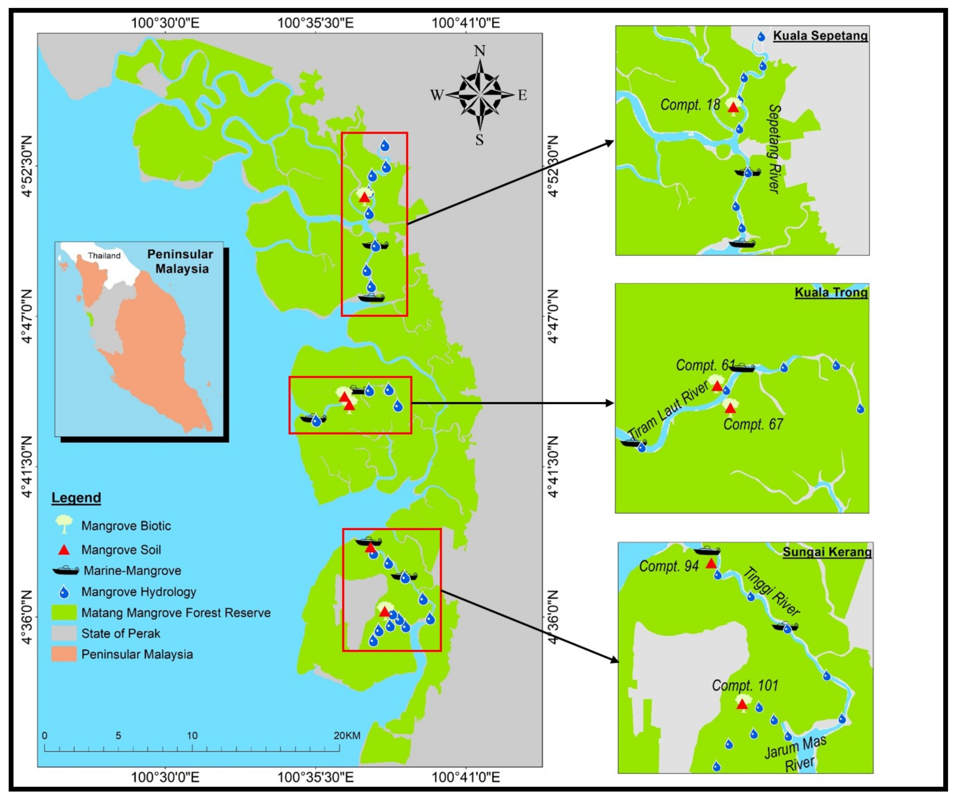
2.1. Description of Site

This study was conducted in the Matang Mangrove Forest Reserve (MMFR). The MMFR is located in the Northern region of Peninsular Malaysia; it lies from the latitudes 4°32′10.81″ N to 4°56′03.54″ N, and from longitudes 100°28′33.26″ E to 100°37′40.54″ E; stretches from Kuala Gula in the north to Bagan Panchor in the south. The MMFR is the largest mangrove forest in Peninsular Malaysia, with a total area of 40,288 ha [49]. This forest consists of 19 patches, which are segmented by numerous large and small rivers; they are joined with the coastal areas of the Malacca Straits in the West, with a total of 108 compartments. The Matang mangroves are divided into four management zones, namely (1) Kuala Sepetang North, (2) Kuala Sepetang South, (3) Kuala Trong, and (4) Sungai Kerang (Figure 1).

2.2. Variables

To identify the parameters that influence mangrove ecosystem health, we used different datasets from Faridah-Hanum et al. [1]. These data have been measured and sampled from 2015 to 2016. In their study, eight variables (aboveground biomass (AGB), abundance of crab, soil nitrogen (N), soil carbon (C), number of phytoplankton species, number of diatom species, dissolved oxygen (DO) and turbidity) were chosen from 43 variables via principal component analysis (PCA). Later, all 8 variables were integrated and analysed using ArcGIS software version 10.3 for geostatistical analysis. Consequently, we interpolated all the variables obtained from all the sampling points to represent the status of mangrove health in the MMFR. A linear weight combination was used to show the distribution map. For validation, we used the vegetation status derived from the vegetation indices analysis conducted by Rhyma et al. [13]. Figure 2 shows the workflow of the methodology performed in this study.

In this present study, a total of 56 sampling points (Figure 1) were selected for the purpose of estimating mangrove ecosystem health using geostatistical analysis. These sampling points were selected based on the classification of disturbance levels, namely least disturbed, moderately disturbed and highly disturbed from previous work [1,22].

All the variables were then converted into spatial data. In order to do this, attributes for all the variables were given coordinates, represented in points; they were saved in the vector format of shapefile (*.shp) so that the data could be analysed using the geostatistical tools of ArcGIS software version 10.3. During the sampling process, coordinates were taken by using the Global Positioning System (GPS) Garmin 72H with standardised units as in Kertau Rectified Skew Orthomorphic (RSO). Since the sampling points for four variables—AGB, crab abundance, soil C and soil N—were located under a dense canopy, we collected two coordinates; first, at the point where the boat reached the river bank, and the second at the point where we collected the samples within. From the first point, we used measuring tape and a compass to obtain the distance and direction to reach the second point. Both coordinates were checked for fore bearing and back bearing with distance conducted in AutoCAD software version 2018. This was to ensure good accuracy of the GPS reading. All the variables collected differ in terms of the number of samples and locations, as presented in

Table 1. Variables, number of samples and number of sampling points collected within the MMFR *.

Variables		Number of Samples (Number of Sampling Points)
		Kuala Sepetang	Kuala Trong	Sungai Kerang
Mangrove biotic integrity	Aboveground biomass (tonnes/ha)	193 (5)	33 (5)	144 (5)
	Crab abundance	68 (5)	191 (5)	352 (5)
Mangrove soil	Soil carbon (%)	12 (3)	12 (3)	24 (6)
	Soil nitrogen (%)	12 (3)	12 (3)	24 (6)
Marine mangrove	Number of phytoplankton species	123 (2)	121 (2)	81 (2)
	Number of diatom species	87 (2)	88 (2)	56 (2)
Mangrove hydrology	Dissolved oxygen (mg/L)	16 (8)	11 (5)	22 (11)
	Turbidity (NTU)	16 (8)	9 (5)	22 (11)

* Number in brackets shows the number of sampling points for each variable in the respective regions.

.

2.3. Geostatistical Analysis

For prediction with geostatistical analysis, the general formula used is as in Equation (1).

$$\widehat{z}\left(x_0\right)={\displaystyle \sum }_{i=1}^n{\lambda }_{i}z\left(x_i\right)$$

(1)

where $\widehat{z}$ is the predicted value of the primary variable at the point of interest x₀, λ_i is the weight assigned to the sampled point, and $n$ represents the number of sampled points used for the prediction [28].

In this study, a geostatistical analysis was performed using the Geostatistical Analyst extension available in ArcGIS software version 10.3 to generate prediction distribution maps. Prior to that, the distribution of the original sampling location needed to be checked if there were outliers. Gidey [38] and Bhunia et al. [39] recommended that this could be confirmed by checking the skewness adjacent to 0, and the kurtosis near 3. From our examination, AGB, crab abundance, soil C, soil N, and turbidity have a symmetric distribution of sampling points, while the number of phytoplankton species, number of diatom species and DO do not. Therefore, normalisation of log transformation was applied on soil C, the number of phytoplankton species and turbidity variables due to the asymmetric distribution.

Once all the variables were normalised, Kriging was performed. The ordinary Kriging (OK) method was chosen to simplify the original sampling density and ensure the accuracy of prediction, as suggested by Omran [37]. To estimate the health of the mangrove ecosystem, we chose the output surface type of prediction by default [50]. To examine the accuracy of the predicted distribution map, all the variables were tested with 11 semivariogram models viz. circular, spherical, tetraspherical, penstraspherical, exponential, gaussian, rational quadratic, hole effect, k-bessel, j-bessel and stable. This step is known as the cross-validation technique. The results then appeared as a prediction map and a graph presenting the cross-validation of the variables, which summarised and interpreted mangrove ecosystem health. Further, the results provide samples, the mean (ME), the root mean square error (RMSE), the mean standardised error (MSE), the RMS standardised error (RMSSE), and the average standard error (ASE). We then checked the ME, the RMSE and the RMSSE to choose the best-fit model. The prediction is considered good and precise if the ME is nearing 0, the RMS nearing 0, and the RMSSE nearing 1 [38,39,40].

The mean error (ME), the root mean square error (RMSE) and root mean square standardised error (RMSSE) were obtained using ArcGIS interpolation techniques [51]. The equation for the ME, the RMSE and the RMSSE is presented in Equations (2)–(4), respectively.

$$\mathrm{ME}=\frac{{{\displaystyle \sum }}_{i=1}^n(\widehat{Z}\left(s_i\right)-\left(z{s}_i\right))}{n}$$

(2)

$$\mathrm{RMSE}=\sqrt{\frac{{{\displaystyle \sum }}_{i=1}^n{(\widehat{Z}\left(s_i\right)-\left(z{s}_i\right))}^2}{n}}$$

(3)

$$\mathrm{RMSSE}=\frac{{{\displaystyle \sum }}_{i=1}^n(\widehat{Z}\left(s_i\right)-\left(z{s}_i\right))/\sigma \left(s_i\right)}{n}$$

(4)

The semivariogram depicts the spatial autocorrelation of the measured sample points characterise by the nugget effect, the sill and the range [52]. The nugget effect describes the small-scale variability of the data and measurement errors that appear spatially random at the scale of investigation and is the extrapolated y-axis intercept of the semivariogram [53,54,55,56]. The sill represents the maximum variability of measured points, and the range is the maximum distance up to which a variable is spatially autocorrelated [53,54]. The nugget-to-sill ratio therefore represents the degree of spatial dependency which the smaller ratios indicate greater proportions of spatially dependent variation [53,54]. This ratio is an important feature of semivariogram [54]. This method was suggested by Behrens et al. [53], and Engström and Esbensen [54], and was a useful method to assess the overall observable variability represented by the sill.

2.4. Reclassification and Standardisation

Since the resulting map for all the variables estimated through Kriging was in the raster format, we needed to reclassify and standardise the map for ease of analysis [57,58,59]. All the variables were reclassified into 5 classes following the mangrove quality sub-index (MQIS_i); where i is the type of variable [1], viz. 1 (worst; MQIS_i < −1.5), 2 (bad; −1.5 ≤ MQIS_i ≤ −0.5), 3 (moderate; −0.5 ≤ MQIS_i ≤ 0.5), 4 (good; 0.5 ≤ MQIS_i ≤ 1.5), and 5 (excellent; MQIS_i > 1.5). Thus, the Natural Breaks (Jenks) reclassification method was used to classify all the variables into five classes of MQIS_i relative basis [60].

2.5. Linear Weight Combination Model

In order to determine the ecosystem health of the entire MMFR, we applied the linear weight combination (Equation (5)) to all the variables. Prior to that, the weightage of 12% was prorated for 7 variables, viz. crab abundance, soil C, soil N, number of phytoplankton sp., number of diatom sp., DO, and turbidity, assuming all the variables have equal influences on mangrove ecosystem health. We gave 16% weightage to AGB, which is the highest among all the variables. This is the reason: the vegetation status used by Faridah-Hanum et al. [1] to calculate AGB was the main indicator in determining the condition of the mangrove. Vegetation and vegetation health is the level of primary producers within ecosystems [61]. A previous study by Wang et al. [62] and Mouat [63] suggested ecosystem vigour as part of the parameters to determine ecosystem health which was convenient to use the vegetation index of remote sensing to apply on the large scale. Thus, we used the vegetation indices from Rhyma et al. [13] to validate the mangrove ecosystem health distribution map generated in this present study. Different variables may have different influences in determining mangrove ecosystem health. In addition, different management regimes of mangroves [49,64] may also influence the ecosystem’s health determination. This limitation was not discussed in our current work; however, future works will encompass the weightage of variables based on ranking order while considering the different management regimes for mangrove ecosystem health. Thus, the weightage was calculated by using the arithmetic operation of raster data (multiplication) and the operation is expressed in Equation (6). Thus, the range of combined MQIS_i was interpreted as 1 (worst; MQI < −1.5), 2 (bad; −1.5 ≤ MQI ≤ −0.5), 3 (moderate; −0.5 ≤ MQI ≤ 0.5), 4 (good; 0.5 ≤ MQI ≤ 1.5), and 5 (excellent; MQI > 1.5).

$$S={\displaystyle \sum }_i^{n}WiXi$$

(5)

where $WiXi$ is the ith factor weight, and the ith factor is the criterion score.

(16 × AGB) + (12 × crab abundance) + (12 × soil C) + (12 × soil N) +
(12 × no. of phytoplankton) + (12 × no. of diatom) + (12 × DO) + (12 × turbidity)

(6)

3. Results and Discussion

3.1. Best-Fit Model of Geostatistical Analysis

Table 2. Descriptive statistics of mangrove quality variables.

Variables	Minimum	Maximum	Mean	Median	SD	Skewness	Kurtosis
AGB (tonne/ha)	7.83	61.32	30.047	24.24	16.322	0.237	2.23
Crab abundance	3	91	40.733	38	26.196	0.234 *	2.26
Soil C (%)	6.527	20.908	10.711	9.0787	4.5865	1.080 (0.660)	3.01
Soil N (%)	0.113	0.648	0.34942	0.3215	0.17625	0.230 *	1.90
No. of phytoplankton sp.	57	120	94.167	100.5	23.439	−0.591 (−0.834)	2.03
No. of diatom sp.	51	84	69.333	73.5	12.956	−0.461 *	−0.46
DO (mg/L)	2.215	5.655	4.0135	4.25	1.0155	−0.334 *	1.87
Turbidity (NTU)	8.48	116.03	44.026	33.346	27.995	0.654 (0.409 *)	2.76

* The distribution is approximately symmetric, indicating near normal distribution. Values in brackets are after normalisation.

shows the mangrove quality variables of mangrove ecosystem health. Variables with skewness falling between −1 and −0.5 or between 0.5 and 1 (soil C, no. of phytoplankton species and DO) are normalised for further geostatistical analysis.

Prediction performances were assessed by cross-validation, which examined the accuracy of the estimated distribution map. Additionally, the spatial autocorrelation of the measured sample points was examined based on the ratio between the nugget and sill. The nugget effect can be attributed to measurement errors or spatial sources of variation at distances smaller than the sampling interval or both [52]. Bhunia et al. [39] suggested that the ratio values of <0.25, 0.25–0.75 and > 0.75 show strong, moderate and weak spatial autocorrelation, respectively. Although three variables of our study are characterised by moderate (soil C and turbidity) and weak (number of phytoplankton spp.) autocorrelation, which indicates that the locations of sampling points are farther apart, our future work will encompass the scales of spatial variation in data collection. However, in this study, we proceed to estimate mangrove ecosystem health with the existing original data. The methodology and steps of geostatistical analysis undertaken in this study will be useful for our future work in estimating mangrove ecosystem health with good accuracy by understanding the spatial variation in sample points [39].

Table 3. Best-fit model of semivariogram for OK interpolation.

Variables	Model	Nugget/Sill	Prediction Errors
			ME	RMSE	RMSSE
AGB (tonne/ha)	Hole Effect	1.108	−0.3397	14.8418	0.9953
Crab abundance	Spherical	0	−0.1055	9.2213	0.9050
Soil C (%)	Circular	0.327	−0.0283	2.7024	0.9651
Soil N (%)	Exponential	0.169	−0.0005	0.0993	0.9762
No. of phytoplankton sp.	Gaussian	0.086	−0.0165	10.7670	1.3591
No. of diatom sp.	Hole Effect	0.032	−0.1975	4.3751	0.9919
DO (mg/L)	Stable	1.348	−0.0001	0.6430	0.9348
Turbidity (NTU)	Rational Quadratic	0	1.1194	12.6746	0.7975

summarises the semivariogram model of mangrove ecosystem health variables using hole effect, spherical, circular, exponential, Gaussian, stable, and rational quadratic models. All models were chosen based on the overall prediction accuracy obtained through examination of the ME that is nearing 0, the RMSSE nearing 1, and the smallest RMSE from all the 11 models tested with semivariogram. Later, these models were used to predict and map the spatial distribution of all the variables of the entire MMFR.

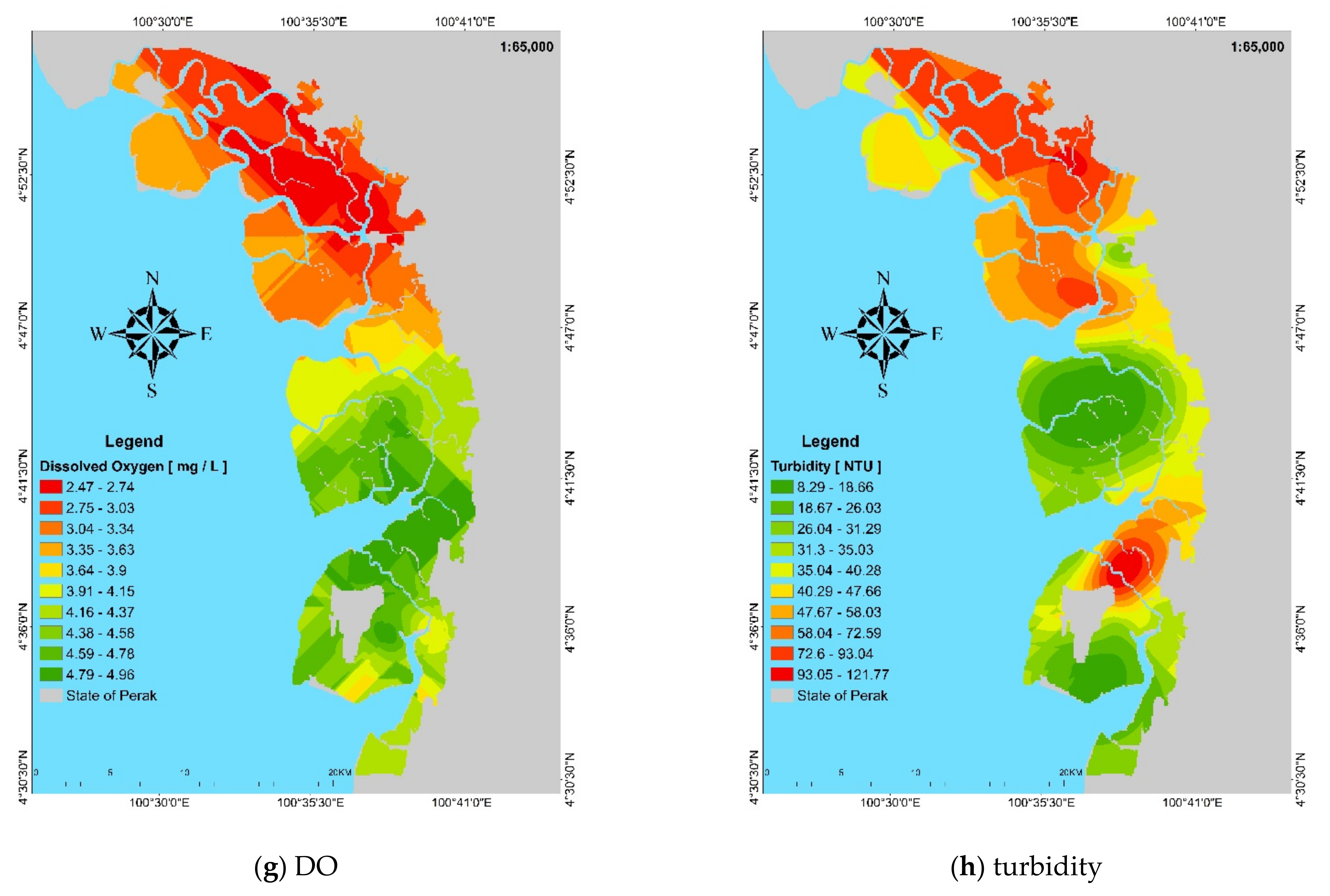
3.2. Geospatial Distribution Map

The geospatial distribution of mangrove ecosystem health was spatially autocorrelated as a result of the interpolation using eight selected variables. Figure 3 a–h show the predicted values for all the variables. To reflect this spatial prediction autocorrelation of the selected variables over the entire MMFR, recent images subsequent to the completion of data collection in Rhyma et al. [13] were compared and observed from a geospatial distribution map produced in this study. This procedure was suggested by Palmer et al. [65], who opined that guiding images can be useful information to verify a healthy ecosystem.

The excellent quality of AGB (MQIS_i > 1:5) is recorded in some parts of Kuala Sepetang (North East of the landward region) and Sungai Kerang (South region) with 34.07–39.67 tonnes/ha, while the worst quality of AGB (MQIS_i < −1.5) is recorded in the middle of the MMFR covering Kuala Trong in the seaward region, and the Northern part (seaward region) of Kuala Sepetang with 17.35–29.89 tonnes/ha. In our on-site observations of the ground truth, there were high tree compositions within many transects in the Kuala Sepetang and Sungai Kerang areas. This was the positive result of the tree harvesting rotation system carried out in the MMFR. Most areas of Kuala Sepetang, especially in the landward region, underwent timber harvesting in the year 2006 [48,63]. According to our data collected in the year 2016, most of the areas had been replanted and regenerated with new trees aged approximately 10 years. The southern part of Sungai Kerang is designated as Virgin Jungle Reserve (VJR), which means no timber harvesting is permitted within that area. This is the reason the southern part of Sungai Kerang has a high AGB value. These situations are consistent with a study conducted by Imani et al. [66], the findings of which reveal that the forest structure has greater effects on the aboveground biomass.

According to Askar et al. [67], and Baghi and Oldeland [68], the NDVI is the right analysis to estimate AGB and is often used in interpreting ecosystem health. On the other hand, Escadafal [69] suggested that the SAVI can be a complementary analysis to the NDVI where the areas studied are characterised by sparse vegetation cover that results in a bright soil background and creates a soil noise signal. Observations of Rhyma et al. [13] show that Sungai Kerang has low NDVI and SAVI values in the seaward region, and this is in line with a spatial prediction autocorrelation derived from the OK method using the Hole Effect semivariogram model, as shown in Figure 3a. High AGB observed is in the landward region of Kuala Sepetang and southern part of Sungai Kerang, which also have high NDVI (0.31—Kuala Sepetang; 0.64—Sungai Kerang) and SAVI values (0.54—Kuala Sepetang; 1.11—Sungai Kerang).

Vegetation distribution exerts a significant influence on crab abundance. Lindquist et al. [70] described crabs prefer seeds, propagules, fruits, seedlings and leaf litter as their sources of food. Cannicci et al. [71] suggested that the spatial prediction autocorrelation of mangrove crabs is commonly associated with tree zonation and abiotic factors such as ground temperature and soil granulometry. Our predicted results indicate an excellent quality of crab abundance (MQIS_i > 1:5) in some parts of Sungai Kerang, with 59–81 crabs observed; the worst quality of crab abundance (MQIS_i < −1.5) mostly occurs in the seaward regions of Kuala Trong stretching towards Kuala Sepetang, with 3–23 crabs observed as Figure 3b. By observing the values in the NDVI and SAVI maps [13], VJR and land with matured mangrove trees (mostly aged more than 20 years) are identified as areas of excellent crab abundance. Within this physical environment, there are rich food sources for the crabs. In addition, there is no disturbance from tree thinning activities go; this is a primary reason Sungai Kerang has excellent crab abundance compared with the other regions. Kuala Sepetang was reported by Perak State Forestry Department as a production forest; thus, there are lots of disturbances from human activities related to timber harvesting operations, and this factor coupled with the upstream anthropogenic activities may have reduced the abundance of crabs [5].

Crab activities contribute to the recycling of nutrients [72,73,74,75]. Qiu et al. [76] describe crab burrowing activities that can promote retention and accumulation of soil C and soil N. Our spatial prediction autocorrelation of soil C as Figure 3c and soil N as Figure 3d are comparable with the spatial prediction autocorrelation of crab abundance distribution, and our study findings are consistent with those of Qiu et al. [76]. Both soil C and soil N are important in the growth and productivity of mangrove species [77]. Compton et al. [78], in their study, suggested that vegetation has no effects on soil nutrients. Faridah-Hanum et al. [1] reported soil C and soil N show a positive relationship with the degree of disturbance in the MMFR; both nutrients increase from the least disturbed sites to the most disturbed sites. The least disturbed sites in their study are characterised by high dense vegetation, and the most disturbed sites are characterised by low dense vegetation as reported in the work of Rhyma et al. [22]. As such, our trends of the spatial prediction autocorrelation of vegetation with soil C and soil N are non-comparable.

For the marine-mangrove variables, spatial prediction autocorrelation shows the seaward region of Kuala Trong throughout Sungai Kerang in the Southern part has an excellent number of phytoplankton species (MQIS_i > −1.5), with an average of 106–120 species. On the other hand, almost all of Kuala Sepetang region is predicted to have the lowest number of phytoplankton sp. with approximately 57–67 species (MQIS_i < −1.5) as Figure 3f. In a study by Faridah-Hanum et al. [1], phytoplankton species are found to be highly distributed in the least disturbed areas. According to the study by Rhyma et al. [13], Kuala Trong has the highest NDVI value (0.65) compared with Sungai Kerang and Kuala Sepetang. The distribution of phytoplankton is subject to environmental conditions of the coastal ecosystem. Nursuhayati et al. [79] and Revilla et al. [80] describe nutrients, turbidity, and salinity influence the number and abundance of phytoplankton species, while Mackey and Currie [81] stress disturbances in the coastal ecosystem affect species diversity and species richness of phytoplankton communities. This might be the reason Kuala Sepetang has the lowest number of phytoplankton sp. due to active timber harvesting operations as well as anthropogenic activities in the upstream region.

Antonelli et al. [82] and Desrosiers et al. [83] explained diatom as a bio-indicator of coastal ecosystems due to their sensitivity to nutrient loadings. In our spatial prediction autocorrelation, an excellent number of diatoms species (MQIS_i > −1.5) are distributed in small parts of Kuala Trong and Sungai Kerang in the seaward region, with 80–88 species as Figure 3f. Our spatial prediction autocorrelation using the OK semivariogram model of the hole effect shows there is an excellent number of diatom species in the middle region of Kuala Sepetang, with the highest number in the seaward region. This prediction contradicts the finding of Faridah-Hanum et al. [1] which describes diatoms are highly distributed in areas with a high level of total dissolved solids, and lowly distributed in areas with high turbidity. There are ongoing timber harvesting operations in Kuala Sepetang, and the area has higher turbidity resulting from erosion materials as well as the upstream anthropogenic activities; this combination of factors might have contributed to the worst number of mangrove-marine variables—the number of phytoplankton sp. and number of diatoms spp. as Figure 3e,f. Farther distances between the locations of sampling points (as mentioned in Section 3.1) may have influenced our spatial prediction autocorrelation.

The availability of aquatic organisms is influenced by conditions of water quality [84,85]. The DO as presented in Figure 3g is predicted to have a pattern similar to that of phytoplankton and diatom, except in the middle part of Kuala Sepetang. However, the spatial prediction autocorrelation of turbidity is slightly different for DO in the upper part of Sungai Kerang (right at the bottom of Kuala Trong), which is predicted to have high turbidity as Figure 3h. Using the Rational Quadratic semivariogram model, the original data were used in predicting turbidity for the entire MMFR; the overall prediction accuracy is low compared with other variables—ME: 1.1194; RMSE: 12.6746; RMSSE: 0.7975 [38,39,40]. This might be the reason for the different trend of turbidity as compared with DO [86].

3.3. Mangrove Ecosystem Health Distribution

In this study, mangrove ecosystem health is assessed using the MQI. The MQI was developed by Faridah-Hanum et al. [1] to determine a baseline of mangrove ecosystem health which took into consideration the mangrove forest, contributing components of a mangrove forest, soil, surrounding marine ecosystem, and hydrology variables. They found three of five types of health classes for three regions of the MMFR are MQI 2 (bad) for Kuala Sepetang, MQI 5 (excellent) for Kuala Trong and MQI 4 (good) for Sungai Kerang. However, their findings were based on selected and accessible sampling locations. With the geostatistical analysis, their findings could be utilised to predict health classes for unsampling locations with distribution areas. As a validation method, the NDVI was used by Faridah-Hanum and colleagues [1].

Vegetation indices have been developed over the last four decades [87]. Over forty vegetation indices have been developed for qualitatively and quantitatively evaluating vegetation covers using spectral measurements of canopy cover [88]. In this study, vegetation indices studies by Rhyma et al. [13] were used to validate and quantify the areas of health distribution prior to their capability to indicate the vigour of vegetation [88]. This method has been successfully applied in previous studies such as Razali et al. [20], Bannari et al. [87], Chellamani et al. [88] and Flores-Cárdenas [89].

Figure 4 shows the combined results of all the variables through weighted overlay after they are standardised into five health classes. Approximately 307.9 ha of the MMFR are predicted to have excellent health (MQI > −1.5), distributed in small parts of Sungai Kerang; 15935.68 ha are predicted to have good health (0.5 ≤ MQI ≤ 1.5), concentrated in Kuala Trong and Sungai Kerang; 5224.34 ha are predicted to have moderate health (−0.5 ≤ MQI ≤ 0.5), distributed in small parts of Kuala Trong and Kuala Sepetang in the middle of the MMFR. Bad (17795.63 ha) and worst (715.55 ha) ecosystem health (MQI < −1.5) occur mainly in areas along the Kuala Sepetang river, which is active with timber harvesting operations and has a high concentration of anthropogenic activities. When the present study is viewed together with the results of previous studies undertaken by Faridah-Hanum et al. [1] and Rhyma et al. [13], all the variables are relevant in evaluating the mangrove health (divided into 3 regions: Kuala Sepetang, Kuala Trong and Sungai Kerang), and they are similar to the trend of the MQI with the NDVI and the SAVI (

Table 4. Vegetation indices and the MQI of the Matang Mangrove Forest Reserve (sources: Faridah-Hanum et al. [1] and Rhyma et al. [13]).

Region	Vegetation Indices [13]		MQI [1]
	NDVI	SAVI
Kuala Sepetang	−0.916667–0.314991	−1.55556–0.545049	MQI 2 (bad)
Kuala Trong	−0.689846–0.652204	−1.15279–1.12794	MQI 5 (excellent)
Sungai Kerang	−0.732505–0.638626	−1.22977–1.10828	MQI 4 (good)

). The results of this study indicate the geostatistical analysis of OK can lead to desired management and facilities distribution for improving the ecosystem health of the MMFR, which can be attained through continual monitoring.

3.4. Limitation of Study

In this study, we faced two main limitations. The first is the model validation, and the second is the performance evaluation of eight (8) variables used with the MQI. Since the study area is managed by different management regimes, each variable’s influence on mangrove ecosystem health determination may vary. Different management regimes practised in this study area characterised the vegetation with different ages due to timber harvesting at 30 years. Before that, thinning is conducted at the ages of 15 and 20, aiming to produce straight timber for charcoal. These uneven forest stand age and density may vary the ecosystem in the respective area. Thus, the ecosystem health obtained from the linear weight combinations may differ slightly from the actual ground conditions. This is because each variable may affect different management regimes differently. All variables can be ranked as the most important to see their performance in evaluating mangrove ecosystem health. Multi-criteria analysis is an alternative to rank all variables [90,91] before mangrove ecosystem health modelled with linear weight combination analysis. In this current work, we are assuming all variables influence mangrove ecosystem health at a similar rate as tested by Faridah-Hanum et al. (2019). These eight (8) variables have been evaluated with principal component analysis (PCA) from 43 variables. In addition, validation with the NDVI in this study to examine vegetation conditions at different management regimes is reflective of the MQI identified in the study area. Lausch et al. [61], Wang et al. [62], and Mouat [63] also explained that the NDVI could be a helpful method to evaluate the health of the ecosystems. In our ongoing study, we aim to differentiate the validation by different stand ages and density while ranking the important variables with multi-criteria analysis.

4. Conclusions

This study was conducted to evaluate the health of the mangrove ecosystem for the entire MMFR with respect to spatial variation. Variables chosen for this evaluation are acceptable according to the study by Faridah-Hanum et al. [1]. The OK geostatistical analysis has successfully estimated the values of the mangrove ecological variables, with the best-fit model of hole effect for AGB and number of diatom sp., spherical for crab abundance, circular for soil C, exponential for soil N, Gaussian for the number of phytoplankton sp., stable for DO, and rational quadratic for turbidity, in terms of a good ME, RMSE and RMSSE. The best-fit model of semivariogram shows the accuracy of interpolation. The prediction geospatial distribution map produced, and accuracy assessment conducted with vegetation indices from Rhyma et al. [13] show that the ecosystem health of the MMFR is: excellent in small parts of Sungai Kerang; good in the Kuala Trong and Sungai Kerang regions; moderate in some areas of Kuala Trong; and bad in Kuala Sepetang region.

The outcomes of this study may provide valuable insights into mangrove ecosystem health and factors contributing to excellent biological growth. The information can be utilised to formulate appropriate management plans, particularly for conserving the MMFR to the highest level of health. The application of geospatial modelling could be a useful tool for managers in making decisions associated with mangrove management such as intensity of rehabilitation and extent of resource protection. Modelling applied in this study can also be used for monitoring long-term changes in mangrove quality, and hence overall health in the years to come.

References

1. Faridah-Hanum, I.; Yusoff, F.M.; Fitrianto, A.; Ainuddin, N.A.; Gandaseca, S.; Zaiton, S.; Nurhidayu, S.; Roslan, M.K.; Hakeem, K.R.; Shamsuddin, I.; et al. Development of a comprehensive mangrove quality index (MQI) in Matang mangrove: Assessing mangrove ecosystem health. Ecol. Indic. 2019, 102, 103–117. [Google Scholar] [CrossRef]
2. Thomas, N.; Lucas, R.; Bunting, P.; Hardy, A.; Rosenqvist, A.; Simard, M. Distribution and drivers of global mangrove forest change, 1996–2010. PLoS ONE 2017, 12, e0179302. [Google Scholar] [CrossRef] [PubMed] [Green Version]
3. Richards, D.R.; Friess, D.A. Rates and drivers of mangrove deforestation in Southeast Asia, 2000–2012. Proc. Natl. Acad. Sci. USA 2016, 113, 344–349. [Google Scholar] [CrossRef] [PubMed] [Green Version]
4. Asbridge, E.; Lucas, R.; Accad, A.; Dowling, R. Mangrove response to environmental changes predicted under varying climates: Case studies from Australia. Curr. For. Rep. 2015, 1, 178–194. [Google Scholar] [CrossRef] [Green Version]
5. Ibharim, N.A.; Mustapha, M.A.; Lihan, T.; Mazlan, A.G. Mapping mangrove changes in the Matang mangrove forest using multi temporal satellite imageries. Ocean Coast. Manag. 2015, 114, 64–76. [Google Scholar] [CrossRef]
6. Misra, A.; Murali, M.R.; Vethamony, P. Assessment of the land use/land cover (LU/LC) and mangrove changes along the Mandovi–Zuari estuarine complex of Goa, India. Arab. J. Geosci. 2015, 8, 267–279. [Google Scholar] [CrossRef]
7. Nguyen, H.H. The relation of coastal mangrove changes and adjacent land-use: A review in Southeast Asia and Kien Giang, Vietnam. Ocean Coast. Manag. 2014, 90, 1–10. [Google Scholar] [CrossRef]
8. Nguyen, H.; Mcalpine, C.; Pullar, D.; Johansen, K.; Duke, N.C. Ocean and coastal management the relationship of spatial e temporal changes in fringe mangrove extent and adjacent land-use: Case study of Kien Giang coast, Vietnam. Ocean Coast. Manag. 2013, 76, 12–22. [Google Scholar] [CrossRef]
9. Kirui, K.B.; Kairo, J.G.; Bosire, J.; Viergever, K.M.; Rudra, S.; Huxham, M.; Briers, R.A. Mapping of mangrove forest land cover change along the Kenya coastline using Landsat imagery. Ocean Coast. Manag. 2013, 83, 19–24. [Google Scholar] [CrossRef]
10. Abdullah, S.A.; Nakagoshi, N. Forest fragmentation and its correlation to human land use change in the state of Selangor, peninsular Malaysia. For. Ecol. Manag. 2007, 241, 39–48. [Google Scholar] [CrossRef]
11. Giri, C.; Pengra, B.; Zhu, Z.; Singh, A.; Tieszen, L.L. Monitoring mangrove forest dynamics of the Sundarbans in Bangladesh and India using multi-temporal satellite data from 1973 to 2000. Estuar. Coast. Shelf Sci. 2007, 73, 91–100. [Google Scholar] [CrossRef]
12. Thu, P.M.; Populus, J. Status and changes of mangrove forest in Mekong delta: Case study in Tra Vinh, Vietnam. Estuar. Coast. Shelf Sci. 2007, 71, 98–109. [Google Scholar] [CrossRef]
13. Rhyma, P.P.; Norizah, K.; Hamdan, O.; Faridah-Hanum, I.; Zulfa, A.W. Integration of normalised different vegetation index and soil-adjusted vegetation index for mangrove vegetation delineation. Remote Sens. Appl. Soc. Environ. 2020, 17, 100280. [Google Scholar] [CrossRef]
14. Hamdan, O.; Khairunnisa, M.R.; Ammar, A.A.; Mohd Hasmadi, I.; Khali Aiz, H. Mangrove carbon stock assessment by optical satellite imagery. J. Trop. For. Sci. 2013, 25, 554–565. [Google Scholar]
15. Taureau, F.; Robin, M.; Proisy, C.; Fromard, F.; Imbert, D.; Debaine, F. Mapping the mangrove forest canopy using spectral unmixing of very high spatial resolution satellite images. Remote Sens. 2019, 11, 367. [Google Scholar] [CrossRef] [Green Version]
16. Thomas, N.; Bunting, P.; Lucas, R.; Hardy, A.; Rosenqvist, A.; Fatoyinbo, T. Mapping mangrove extent and change: A globally applicable approach. Remote Sens. 2018, 10, 1466. [Google Scholar] [CrossRef] [Green Version]
17. Son, N.T.; Chen, C.F.; Chen, C.R. Mapping mangrove density from rapideye data in central America. Open Geosci. 2017, 9, 211–220. [Google Scholar] [CrossRef] [Green Version]
18. Conti, L.A.; de Araujo, C.A.S.; Cunha-Lignon, M. Spatial database modeling for mangrove forests mapping; example of two estuarine systems in Brazil. Model. Earth Syst. Environ. 2016, 2, 73. [Google Scholar] [CrossRef]
19. Ghosh, M.K.; Kumar, L.; Langat, P.K. Geospatial modelling of the inundation levels in the Sundarbans mangrove forest due to the impact of sea level rise and identification of affected species and regions. Geomat. Nat. Hazards Risk 2019, 10, 1028–1046. [Google Scholar] [CrossRef]
20. Razali, S.M.; Nuruddin, A.A.; Lion, M. Mangrove vegetation health assessment based on remote sensing indices for Tanjung Piai, Malay Peninsular. J. Landsc. Ecol. 2019, 12, 26–40. [Google Scholar] [CrossRef] [Green Version]
21. Hamdan, O.; Muhamad Afizzul, M.; Samsudin, M. GIS and Remote Sensing for Mangroves Mapping and Monitoring. In Geographic Information System and Science; Rocha, J., Abrantes, P., Eds.; IntechOpen: London, UK, 2019; p. 16. [Google Scholar]
22. Rhyma, P.P.; Norizah, K.; Ismail Adnan, A.M.; Faridah-Hanum, I.; Ibrahim, S. Canopy density classification of Matang mangrove forest reserve using machine learning approach in remote sensing for transect establishment. Malays. For. 2015, 78, 75–86. [Google Scholar]
23. Li, X.; Cheng, X.; Yang, R.; Qiu, Y.; Zhang, J.; Cai, E.; Zhao, L. Validation of remote sensing retrieval products using data from a wireless sensor-based online monitoring in Antartica. Sensors 2016, 16, 1938. [Google Scholar] [CrossRef] [Green Version]
24. Wang, S.; Lin, X.; Ge, Y.; Jin, R.; Ma, M.; Liu, Q.; Wen, J.; Liu, S. Validation of regional-scale remote sensing products in China: From site to network. Remote Sens. 2016, 8, 980. [Google Scholar] [CrossRef] [Green Version]
25. Rhodes, C.J.; Henrys, P.; Siriwardena, G.M.; Whitingham, M.J.; Norton, L.R. The relative value of field survey and remote sensing for biodiversity assessment. Methods Ecol. Evol. 2015, 6, 772–781. [Google Scholar] [CrossRef]
26. Scales, I.R.; Friess, D.A. Pattern or mangrove forest disturbance and biomass removal due to small-scale harvesting in south-western Madagascar. Wetl. Ecol. Manag. 2019, 27, 609–625. [Google Scholar] [CrossRef] [Green Version]
27. Feka, N.Z.; Morrison, I. Managing mangroves for coastal ecosystems change: A decade and beyond of conservation experiences and lessons for and from west-central Africa. J. Ecol. Nat. Environ. 2017, 9, 99–123. [Google Scholar]
28. Li, J.; Heap, A.D. Spatial interpolation methods applied in the environmental sciences: A review. Environ. Model. Softw. 2014, 53, 173–189. [Google Scholar] [CrossRef]
29. Schweiger, A.H.; Iri, S.D.H.; Steinbauer, M.J.; Dengler, J.; Beierkuhnlein, C. Optimizing sampling approaches along ecological Gradients. Methods Ecol. Evol. 2016, 7, 463–471. [Google Scholar] [CrossRef]
30. McLeod, L.; Bharadwaj, L.; Epp, T.; Waldner, C.L. Use of principal components analysis and Kriging to predict groundwater-sourced rural drinking water quality in Saskatchewan. Int. J. Environ. Res. Public Health 2017, 14, 1065. [Google Scholar] [CrossRef] [Green Version]
31. White, J.T.; Hemmings, B.; Fienen, M.N.; Knowling, M.J. Towards improved environmental modelling outcomes: Enabling low-cost access to high-dimensional, geostatistical-based decision-support analyses. Environ. Model. Softw. 2021, 139, 105022. [Google Scholar] [CrossRef]
32. Gupta, A.; Kamble, T.; Machiwal, D. Comparison of ordinary and Bayesian kriging techniques in depicting rainfall in arid and semi-arid regions of north-west India. Environ. Earth Sci. 2017, 76, 512. [Google Scholar] [CrossRef]
33. Tveito, O.E.; Wegehenkel, M.; van der Wel, F.; Dobesch, H. COST Action 719: The Use of Geographic Information Systems in Climatology and Meteorology; EUR-OP: Luxembourg, 2008. [Google Scholar]
34. Webster, R.; Oliver, M. Geostatistics for Environmental Scientists; John Wiley & Sons, Ltd.: Chichester, UK, 2001. [Google Scholar]
35. Mirzaei, R.; Sakizadeh, M. Comparison of interpolation methods for the estimation of groundwater contamination in Andimeshk-Shush Plain, southwest of Iran. Environ. Sci. Pollut. Res. 2016, 23, 2758–2769. [Google Scholar] [CrossRef] [PubMed]
36. Al-Omran, A.M.; Aly, A.A.; Al-Wabel, M.I.; Al-Shayaa, M.S.; Sallam, A.S.; Nadeem, M.E. Geostatistical methods in evaluating spatial variability of groundwater quality in Al-Kharj Region, Saudi Arabia. Appl. Water Sci. 2017, 7, 4013–4023. [Google Scholar] [CrossRef] [Green Version]
37. Omran, E.E. A proposed model to assess and map irrigation water well suitability using geospatial analysis. Water 2012, 4, 545–567. [Google Scholar] [CrossRef] [Green Version]
38. Gidey, A. 2018. Geospatial distribution modelling and determining suitability of groundwater quality for irrigation purpose using geospatial methods and water quality index (WQI) in northern Ethiopia. Appl. Water Sci. 2018, 8, 82. [Google Scholar] [CrossRef] [Green Version]
39. Bhunia, G.S.; Keshavarzi, A.; Shit, P.V.; Omran, E.E.; Bagherzadeh, A. Evaluation of groundwater quality and its suitability for drinking and irrigation using GIS and geostatistics techniques in semiarid region of Neyshabur, Iran. Appl. Water Sci. 2018, 8, 168. [Google Scholar] [CrossRef] [Green Version]
40. Castillo, J.A.A.; Apan, A.A.; Maraceni, T.N.; Salmo, S.G., III. Soil C quantities of mangrove forests, their competing land uses, and their spatial distribution in the coast of Honda Bay Philippines. Geoderma 2017, 293, 82–90. [Google Scholar] [CrossRef]
41. Oliver, M.A.; Webster, R. A tutorial guide to geostatistics: Computing and modelling variograms and kriging. Catena 2014, 113, 56–69. [Google Scholar] [CrossRef]
42. Li, J.; Heap, A. A review of comparative studies of spatial interpolation methods in environmental sciences: Performance and impact factors. Ecol. Inform. 2011, 6, 228–241. [Google Scholar] [CrossRef]
43. Bennett, N.D.; Croke, B.F.W.; Guariso, G.; Guillaume, J.H.A.; Hamilton, S.H.; Jakeman, A.J.; Marsili-Libelli, S.; Newham, L.T.H.; Norton, J.P.; Perrin, C.; et al. Characterising performance of environmental models. Environ. Model. Softw. 2013, 40, 1–20. [Google Scholar] [CrossRef]
44. Chang, Y.H.; Scrimshaw, M.D.; Emmerson, R.H.C.; Lester, J.N. Geostatistical analysis of sampling uncertainty at the Tollesbury Managed Retreat site in Blackwater Estuary, Essex, UK: Kriging and cokriging approach to minimise sampling density. Sci. Total Environ. 1998, 221, 43–57. [Google Scholar] [CrossRef]
45. Brus, D.J.; de Gruijter, J.J. Estimation of non-ergodic variograms and their sampling variance by design-based sampling strategies. Math. Geol. 1994, 26, 437–454. [Google Scholar] [CrossRef]
46. Burrough, P.A.; McDonnell, R.A. Principles of Geographical Information Systems; Oxford University Press: Oxford, UK, 1998. [Google Scholar]
47. Journel, A.G.; Huijbregts, C.J. Mining Geostatistics; Academic Press: London, UK, 1978. [Google Scholar]
48. Kerry, R.; Oliver, M.A. Comparing sampling needs for variograms of soil properties computed by the method of moments and residual maximum likelihood. Geoderma 2007, 140, 383–396. [Google Scholar] [CrossRef]
49. Roslan, A.; Nik Mohd Shah, N.M. A Working Plan for the Matang Mangrove Forest Reserve, Perak: The First 10-Year Period (2010–2019) of the Third Rotation (6th Revision); State Forestry Department of Perak: Ipoh, Malaysia, 2014; p. 229. [Google Scholar]
50. ESRI. 2019a. An Overview of ArcMap extension: ArcGIS Geostatistical Analyst. Available online: https://desktop.arcgis.com/en/arcmap/latest/extensions/main/about-arcgis-for-desktop-extensions.htm (accessed on 7 January 2019).
51. Esri. 2020. Available online: https://pro.arcgis.com/en/pro-app/2.8/tool-reference/geostatistical-analyst/cross-validation.htm (accessed on 18 June 2020).
52. ESRI. 2019. Available online: https://pro.arcgis.com/en/pro-app/help/analysis/geostatistical-analyst/understanding-a-semivariogram-the-range-sill-and-nugget.htm (accessed on 11 February 2020).
53. Behrens, T.; Viscarra Rossel, R.A.; Kerry, R.; MacMillan, R.; Schmidt, K.; Lee, J.; Scholten, T.; Zhu, A.-X. The relevant range of scales for multi-scale contextual spatial modelling. Sci. Rep. 2019, 9, 14800. [Google Scholar] [CrossRef] [Green Version]
54. Engström, K.; Esbensen, K.H. Variographic assessment of total process measurement system performance for a complete ore-to-shipping value chain. Minerals 2018, 8, 310. [Google Scholar] [CrossRef] [Green Version]
55. Viscarra Rossel, R.A.; Mcbratney, A.B. Soil chemical analytical accuracy and costs: Implications from precision agriculture. Aust. J. Exp. Agric. 1998, 38, 765–775. [Google Scholar] [CrossRef]
56. Fortin, M.-J. Spatial Statistics in Landscape Ecology; Springer: New York, NY, USA, 1999; pp. 253–279. [Google Scholar]
57. Rhyma, P.P.; Norizah, K. Kriging analysis–optimizing values in unknown areas using known data point. In Proceeding of the International Conference on Sustainable Forest Development in View of Climate Change (SFDCC), Hotel Bangi-Putrajaya, Malaysia, 8–11 August 2016; Nurhidayu, S., Ainuddin, A.N., Nazre, M., Seca, G., Mohd Zaki, H., Lee, S.H., Eds.; Universiti Putra Malaysia: Selangor, Malaysia, 2016. [Google Scholar]
58. Mishra, A.K.; Deep, S.; Choudhry, A. Identification of suitable sites for organic farming using AHP & GIS. Egypt. J. Remote Sens. Space Sci. 2015, 18, 181–193. [Google Scholar]
59. Norizah, K.; Mohd Hasmadi, I.; Kamaruzaman, J. Quantification of least cost path analysis for best forest road planning. Malays. For. 2014, 77, 99–108. [Google Scholar]
60. Bernal, N.A.; DeAngelis, D.L.; Schofield, P.J.; Sealey, K.S. Predicting spatial and temporal distribution of Indo-Pacific lionfish (Pterois volitans) in Biscayne Bay through habitat suitability modeling. Biol. Invasions 2015, 17, 1603–1614. [Google Scholar] [CrossRef]
61. Lausch, A.; Bastin, O.; Klotz, S.; Leitão, P.; Jung, A.; Rocchini, D.; Schaepman, M.E.; Skidmore, A.K.; Tischendorf, L.; Knapp, S. Understanding and assessing vegetation health by in situ species and remote-sensing approaches. Methods Ecol. Evol. 2018, 9, 1799–1809. [Google Scholar] [CrossRef]
62. Wang, Z.; Yang, Z.; Shi, H.; Han, F.; Liu, Q.; Qi, J.; Lu, Y. Ecosystem health assessment of world natural heritage sites based on remote sensing and field sampling verification: Bayanbulak as case study. Sustainability 2020, 12, 2610. [Google Scholar] [CrossRef] [Green Version]
63. Mouat, D.A. Remote Sensing and Ecosystem Health: An Evaluation of Time-Series AVHRR NDVI Data. In Evaluating and Monitoring the Health of Large-Scale Ecosystems; NATO ASI Series; Rapport, D.J., Gaudet, C.L., Calow, P., Eds.; Springer: Berlin/Heidelberg, Germany, 1995; Volume 28. [Google Scholar]
64. Azahar, M.; Nik Mohd Shah, N.M. A Working Plan for the Matang Mangrove Forest Reserve, Perak: Fifth Revision of the 10-Year Period (2000–2009) of the Second Rotation; State Forestry Department of Perak: Ipoh, Malaysia, 2003; p. 319. [Google Scholar]
65. Palmer, M.A.; Bernhardt, E.S.; Allan, J.D.; Lake, P.S.; Alexander, G.; Brooks, S.; Carr, J.; Clayton, S.; Dahm, C.N.; Follstad Shah, J.; et al. Standards for ecologically successful river restoration. J. Appl. Ecol. 2005, 42, 208–217. [Google Scholar] [CrossRef]
66. Imani, G.; Boyemba, F.; Lewis, S.; Nabahungu, N.L.; Calders, K.; Zapfack, L.; Riera, B.; Balegamire, C.; Cuni-Sanchez, A. Height-diameter allometry and above ground biomass in tropical montane forests: Insights from the Albertine Rift in Africa. PLoS ONE 2017, 12, e0179653. [Google Scholar] [CrossRef] [PubMed] [Green Version]
67. Askar; Nuthammachot, N.N.; Phairuang, W.; Wicaksono, P.; Sayektiningsih, T. Estimating aboveground biomass on private forest using Sentinel-2 imagery. J. Sens. 2018, 2018, 6745625. [Google Scholar]
68. Baghi, N.G.; Oldeland, J. Do soil-adjusted or standard vegetation indices better predict above ground biomass of semi-arid, saline rangelands in North-East Iran? Int. J. Remote Sens. 2019, 40, 8223–8235. [Google Scholar] [CrossRef]
69. Escadafal, R. Remote sensing of drylands: When soils come into the picture. Ciência Trópico 2017, 41, 33–50. [Google Scholar]
70. Lindquist, E.S.; Krauss, K.W.; Green, P.T.; O’Dowd, D.J.; Sherman, P.M.; Smith, T.J. Land crabs as key drivers in tropical coastal forest recruitment. Biol. Rev. 2009, 84, 203–223. [Google Scholar] [CrossRef]
71. Cannici, S.; Fusi, M.; Cimo, F.; Dahdouh-Guebas, F.; Fratini, S. Interference competition as a key determinant for spatial distribution of mangrove crabs. BMC Ecol. 2018, 18, 8. [Google Scholar]
72. Otero, X.L.; Araújo, J.M.C., Jr.; Barcellos, D.; Queiroz, H.M.; Romero, D.J.; Nóbrega, G.N.; Neto, M.S.; Ferreira, T.O. Crab bioturbation and seasonality control nitrous oxide emissions in semiarid mangrove forests (Ceará, Brazil). Appl. Sci. 2020, 10, 2215. [Google Scholar] [CrossRef] [Green Version]
73. Wang, J.Q.; Zhang, X.D.; Jiang, L.F.; Bertness, M.D.; Fang, C.M.; Chen, J.K.; Hara, T.; Li, B. Bioturbation of burrowing crabs promotes sediment turnover and carbon and nitrogen movements in an Estuarine Salt Marsh. Ecosystems 2010, 13, 586–599. [Google Scholar] [CrossRef]
74. Mchenga, I.S.S.; Tsuchiya, M. Crab engineering effects on soil organic matter and nutrients flow in subtropical mangroves forest. J. Global Biosci. 2013, 2, 10–16. [Google Scholar]
75. Sherman, P.M. Influence of land crabs Geocarcinus quadratus (Gecarcinidae) on distributions of organic carbon and roots in a Costa Rican rain forest. Rev. Biol. Trop. 2006, 54, 149–161. [Google Scholar] [CrossRef] [Green Version]
76. Qiu, D.; Cui, B.; Yan, J.; Ma, X.; Ning, Z.; Wang, F.; Sui, H.; Bai, J. Effect of burrowing crabs on retention and accumulation of soil carbon and nitrogen in an intertidal salt marsh. J. Sea Res. 2019, 154, 101808. [Google Scholar] [CrossRef]
77. McLeod, E.; Chmura, G.L.; Bouillon, S.; Salm, R.; Björk, M.; Duarte, C.M.; Lovelock, C.E.; Schlesinger, W.H.; Silliman, B.R. A blueprint for blue carbon: Toward an improved understanding of the role of vegetated coastal habitats in sequestering CO2. Front. Ecol. Environ. 2011, 9, 552–560. [Google Scholar] [CrossRef] [Green Version]
78. Compton, J.E.; Boone, R.D.; Motzkin, G.; Foster, D.R. Soil carbon and nitrogen in a pine-oak sand plain in central Massachusetts: Role of vegetation and land-use history. Oceologia 1998, 116, 536–542. [Google Scholar] [CrossRef]
79. Nursuhayati, A.S.; Yusoff, F.M.; Sharrif, M. Fisheries and aquatic science. J. Fish. Aquat. Sci. 2013, 4, 480–493. [Google Scholar]
80. Revilla, M.; Franco, J.; Bald, J.; Borja, Á.; Laza, A.; Seoane, S.; Valencia, V. Assessment of the phytoplankton ecological status in the Basque coast (northern Spain) according to the European water framework directive. J. Sea Res. 2009, 61, 60–67. [Google Scholar] [CrossRef]
81. Mackey, R.L.; Currie, D.J. The diversity-disturbance relationship: Is it generally strong and peaked? Ecology 2001, 82, 3479–3492. [Google Scholar]
82. Antonelli, M.; Wetzel, C.E.; Ector, L.; Teuling, A.J.; Pfister, L. On the potential for terrestrial diatom communities and diatom indices to identify anthropic disturbance in soils. Ecol. Ind. 2017, 75, 73–81. [Google Scholar] [CrossRef]
83. Desrosiers, C.; Leflaive, J.; Eulin, A.; Ten-Hage, L. Bioindicators in marine waters: Benthic diatoms as a tool to assess water quality from eutrophic to oligotrophic coastal ecosystems. Ecol. Ind. 2013, 32, 25–34. [Google Scholar] [CrossRef]
84. Oelsner, G.P.; Stets, E.G. Recent trends in nutrient and sediment loading to coastal areas of the conterminous U.S.: Insights and global context. Sci. Total Environ. 2019, 654, 1225–1240. [Google Scholar] [CrossRef]
85. Hanrahan, G. Key Concepts in Environmental Chemistry; Elsevier: Amsterdam, The Netherlands, 2012; p. 384. [Google Scholar]
86. Johnstons, K.; ver Hoeft, J.M.; Krivoruchko, K.; Lucas, N. Using ArcGIS Geostatistical Analyst (Vol. 380); Redlands: Esri, CA, USA, 2001. [Google Scholar]
87. Bannari, A.; Morin, D.; Bonn, F.; Huete, A.R. A review of vegetation indices. Remote Sens. Rev. 1995, 13, 95–120. [Google Scholar] [CrossRef]
88. Chellamani, P.; Singh, C.P.; Panigrahy, S. Assessment of the health status of Indian mangrove ecosystems using multi temporal remote sensing data. Trop. Ecol. 2014, 55, 245–253. [Google Scholar]
89. Flores-Cárdenas, F.; Millán-Aguilar, O.; Díaz-Lara, L.; Rodríguez-Arredondo, L.; Hurtado-Oliva, M.A.; Manzano-Sarabia, M. Trends in the normalized difference vegetation index for mangrove areas in Northwestern Mexico. J. Coast. Res. 2018, 34, 877–882. [Google Scholar] [CrossRef]
90. Sheppard, S.R.; Meitner, M. Using multi-criteria analysis and visualisation for sustainable forest management planning with stakeholder groups. For. Ecol. Manag. 2005, 207, 171–187. [Google Scholar] [CrossRef]
91. Wolfslehner, B.; Vacik, H.; Lexer, M.J. Application of the analytic network process in multi-criteria analysis of sustainable forest management. For. Ecol. Manag. 2005, 207, 157–170. [Google Scholar] [CrossRef]
Figure 1. Map of study area in the MMFR showing original sampling point.
Forests 13 01185 g001
Figure 2. Workflow of methodology undertaken in this study.
Forests 13 01185 g002
Figure 3. Spatial interpolation of (a) AGB, (b) crab abundance, (c) soil C, (d) soil N, (e) no. of phytoplankton species, (f) no. of diatom species, (g) DO, and (h) turbidity.
Forests 13 01185 g003aForests 13 01185 g003bForests 13 01185 g003c
Figure 4. Mangrove ecosystem health classification based on LWC.
Forests 13 01185 g004