Article

Gap-Scale Disturbance Patterns and Processes in a Montane Pinus palustris Woodland

Department of Geography, University of Alabama, Tuscaloosa, AL 35487, USA
*
Author to whom correspondence should be addressed.
Forests 2022, 13(8), 1169; https://doi.org/10.3390/f13081169
Submission received: 22 June 2022 / Revised: 19 July 2022 / Accepted: 21 July 2022 / Published: 23 July 2022
(This article belongs to the Section Forest Ecology and Management)

Abstract

:
Gap-scale disturbances drive successional and structural development patterns in most forest ecosystems. Although fire-maintained Pinus palustris woodlands are less light limited than closed canopy forests, gap-scale disturbance processes may still influence successional and developmental pathways. We quantified biophysical characteristics of 50 canopy gaps in a montane Pinus palustris woodland to analyze gap-scale disturbance patterns and processes. We found most gaps (64%) were caused by the death of a single tree. Snag-formed gaps were most common (38%) followed by snapped stems (32%). We hypothesized that insect-induced mortality, perhaps in combination with drought periods, resulted in the high frequency of snag- and snapped stem-formed gaps. We did not find significant differences in gap size or shape based on gap formation or closure mechanisms. Most gaps (74%) were projected to close by lateral crown expansion of gap perimeter trees. We hypothesized most gaps projected to close via subcanopy recruitment would be captured by a P. palustris stem. The majority of gaps were small and gap frequency declined with increased gap size. We found gaps were significantly clustered through the woodland at distances of 8–36 m from gap edge to gap edge but were randomly distributed beyond 36 m.

1. Introduction

All forests are subject to disturbance events which influence stand development patterns and successional pathways. The frequency, magnitude, and spatial extent of these disturbances range from infrequent, catastrophic, stand-wide events to frequent, gap-scale occurrences [1,2]. Localized canopy disturbance events that result from the mortality of small groups of trees, single canopy trees, or even just large branches from canopy dominant stems are the most common natural canopy disturbances in closed canopy forests [3,4]. These gap-scale disturbances initiate structural changes associated with older stands by increasing large woody debris inputs, releasing understory trees from overstory competition resulting in complex vertical stratification of tree crowns, promoting multi-aged structures, and allowing for branch extension and larger tree crowns, among other processes [1,5,6]. Gap-scale disturbance events may also influence species composition patterns via gap-phase succession [7,8,9,10]. At the stand-level, gap-scale disturbances may result in a patchwork mosaic of microsites that support different tree species, tree ages, tree sizes, or stem densities [3,4,11]. By altering fine-scale biophysical conditions, gap-scale canopy disturbances modify heterogeneity and biodiversity in forested ecosystems [12,13].
Fire-maintained Pinus palustris stands throughout the southeastern USA generally exist in savanna or woodland structures. In contrast to closed canopy stands, savanna and woodland ecosystems are not as light limited [14,15]. Nonetheless, research has established that canopy gap disturbances are important in the regulation of ecosystem processes, structural development, and succession in P. palustris savannas and woodlands [14,16,17]. Canopy gap-induced increased insolation in the understory has been shown to improve growth, establishment, and recruitment of P. palustris seedlings and saplings [18,19,20]. Small-sized P. palustris stems are often spatially clustered within canopy gaps [21,22] and ultimately, gap-scale disturbance processes may result in complex stand structures and multiple age classes in these ecosystems [16,23,24].
Frequent, low-intensity surface fires help maintain P. palustris dominance and woodland or savanna structures [25,26]. Fires also enhance ground flora cover and diversity [27,28,29,30]. Pinus palustris needles are an important fuel source as the relatively monospecific canopy results in a continuous fuel bed of fine fuels with a high resin content [31]. Overstory tree density has been linked to the abundance and spatial distribution of Pinus needle litter [32]; thus, fuel loading and fuel bed continuity may be influenced by canopy gap disturbances that modify local overstory tree density patterns [33,34]. These modifications may influence fine-scale fire behavior and subsequently fire effects.
Prior studies have examined gap-scale disturbance processes in P. palustris ecosystems of the USA Coastal Plain (e.g., [14,16,22,23]). However, no studies have quantified canopy gap patterns and processes in montane P. palustris woodlands. Pinus palustris ecosystems on the Coastal Plain and montane stands of the Appalachian Highlands are distinct and differ in stand structure and species composition [35,36,37]. Pinus palustris stands on the relatively flat to gently rolling Coastal Plain typically exist as savannas with relatively low tree density and basal area values. In contrast, montane P. palustris stands of the topographically complex Appalachian Highlands more frequently occur as woodlands with higher tree density and greater basal area [19,38,39]. As a result, Coastal Plain P. palustris savannas are less light limited than woodlands and thus canopy disturbance processes may be comparatively more important in these woodland ecosystems. The overarching goal of our research was to quantify gap-scale disturbance patterns and processes in a montane P. palustris woodland. Our specific objectives were to: (1) examine canopy gap formation mechanisms and quantify gap characteristics, (2) document gap closure mechanisms and canopy recruit patterns, (3) examine the impacts of canopy gaps on species composition and stand structure, and (4) quantify the frequency, size, and spatial distribution of canopy gaps through a montane P. palustris woodland.

2. Materials and Methods

2.1. Study Site

This study was conducted in the Reed Brake Research Natural Area on the Oakmulgee Ranger District of Talladega National Forest, Alabama, USA. A management priority on the district is the restoration and maintenance of Pinus palustris woodland ecosystems [40]. In 1975, the Reed Brake Research Natural Area was established on the Oakmulgee Ranger District because it represented typical forest conditions of the Fall Line Hills [41]. The natural area is 242 ha and contains fire-maintained P. palustris woodlands that were established in the 1930s prior to federal land acquisition. Elevation ranges from 90–155 m above mean sea level and the topography is complex and characterized by steep slopes and narrow ridges. The Fall Line Hills are a transition zone between the Appalachian Highland physiographic provinces and the Coastal Plain [42]. The region supports species characteristic of both Coastal Plain and Appalachian Highland forest communities [43,44,45]. The study site occurs within what Harper [46] classified as the central Pinus palustris region. In this region, P. palustris-dominated woodlands occur on fire-maintained ridgetops, upper slopes, and south-to-west facing middle slope positions. On more mesic sites, Quercus and other hardwood species co-occur with Pinus taeda [2,35,43].
The climate of the study area is classified as humid mesothermal, with long, hot summers and short, mild winters [47]. The average yearly precipitation is 1376 mm, with the highest mean precipitation in February (138 mm) and the lowest mean precipitation in October (86 mm). The average yearly temperature is 17.1 °C, and the mean temperature for January and July is 6.5 °C and 26.9 °C, respectively (30-year normal, [48]). The soil parent materials consist of undifferentiated marine sediments of the Cretaceous age Tuscaloosa Group. Soils of the study site are mainly the Maubila–Smithdale complex [49]. The Maubila soil series is moderately well drained with a ca. 5 cm deep flaggy loam A horizon and clay Bt and C horizons. The Smithdale series is well drained with Ap and E horizons of sandy loam to 33 cm deep and a Bt1 horizon of sandy clay loam and a Bt2 horizon of sandy loam [49].

2.2. Field Methods

To quantify non-gap forest composition and structure, we sampled twenty 0.05-ha circular reference plots in June 2021. Reference plots were installed and inventoried in the same Forest Service-delineated compartment in the Reed Brake Research Natural Area to ensure similar biophysical site conditions, disturbance, and management history. Reference plots were interspersed with canopy gap plots and care was taken to be sure no part of the reference plot was within or bordering a canopy gap. Here, P. palustris is dominant on upper slopes, and on south to west facing mid-slopes, while lower slopes are more often dominated by hardwood species [36,44]. Therefore, canopy gaps and reference plots were only sampled on upper slopes and at south to west facing mid-slope positions. On each reference plot, all trees (live woody stems > 10 cm diameter at breast height (dbh, 1.37 m above the root collar)) were identified by species and dbh and crown class were recorded. Crown class categories (dominant, co-dominant, intermediate, overtopped) were determined by examining the direction and amount of light intercepted by the tree crown [1]. Saplings (live woody stems ≥ 1 m height, ≤10 cm dbh) were tallied by species. Seedlings (live woody stems < 1 m in height) were tallied by species in a 10 m2 nested subplot located in the center of the 0.05 ha reference plot. Percent ground cover was estimated for rocks, gravel, bare ground, coarse woody debris (CWD, deadwood with a diameter ≥ 10 cm), fine woody debris (FWD, dead wood with a diameter < 10 cm), Pinus litter, hardwood litter, grass, and forb cover to the nearest 1% [50,51]. Litter depth was recorded to the nearest 0.01 cm at nine locations in the plot, one at plot center, and one at 6.31 m from plot center and 12.62 m from plot center in each cardinal direction. For each plot, the slope gradient, slope aspect, microscale curvature (linear, concave, convex), and topographic position (ridge, shoulder, backslope) were recorded.
Canopy gaps (n = 50) were located while walking transects through P. palustris dominated stands. Transects were subjectively established on ridgetops and upper-slope positions and to avoid old skid trails. To be sampled, canopy gaps had to meet two criteria: (1) a discernable void in the canopy caused by the removal of a canopy tree and (2) the presence of a gapmaker (i.e., the dead tree or trees that caused the canopy gap to form). Each canopy gap along the transects that met these criteria was sampled. Canopy gap voids that did not contain visible gapmakers were not sampled since we could not ascertain if they were created by the death of canopy trees or were open portions of the woodland canopy unassociated with tree mortality (i.e., microsites long devoid of tree cover). Likewise, if a canopy gap had more than one gapmaker of the same species but in different decay classes, the canopy void was not sampled. Gapmakers of the same species with different decay classes may have resulted from different canopy disturbance events, which would confound the effects of each discrete disturbance [52].
For each canopy opening, we sampled the observed and expanded gap areas. The observed gap was defined as the area directly under the canopy void (i.e., unrestricted from above), and the expanded gap was defined as the entire area extending to the bases of the canopy gap perimeter trees [6,53]. Canopy gap length was measured as the greatest distance (i.e., longest axis) of the observed and expanded gaps. The width was the longest distance of the observed and expanded gaps perpendicular to the length. Observed and expanded gap length and width were measured using a hypsometer and transponder. The coordinates for each canopy gap center (i.e., the intersection of gap length and width axes) were recorded using a Trimble Juno T/5 GPS unit. The microscale curvature, topographic position, slope aspect, and slope gradient were also measured for each canopy gap with a clinometer and sighting compass. The number of gap perimeter trees was recorded to determine how many canopy trees had the potential to close the canopy gap through lateral branch growth. The border of each canopy gap plot was defined by the perimeter trees, which were denoted by observing the canopy and determining which tree crowns constituted the boundaries of the gap. The dbh of all trees (woody stems > 10 cm dbh) within the canopy gap were recorded, including perimeter trees. Based on location, each tree was as classified as within the perimeter, expanded, or observed gap. The crown class and species were also recorded for each tree consistent with the methods used on the reference plots. The formation mechanism of each canopy gap was recorded as a snag (standing dead tree with mostly intact crown), snap (broken bole), or uproot (uplifted root network). In the case of canopy gaps with multiple gapmakers, all formation mechanisms were recorded. The dbh (for snags), or the diameter 1.37 m from the root collar (for downed logs), species, and decay class of each gapmaker were recorded. The decay class was assigned based on Ulyshen et al. [54], which was developed specifically for P. palustris. This system includes seven decay classes for downed CWD and five for standing dead wood. The decay classes were used to facilitate the determination of canopy gap formation age. To calculate the average height of the canopy surrounding the canopy gap, the height of four perimeter canopy trees, one in approximately each cardinal direction, was measured using a hypsometer and transponder.
In each canopy gap, saplings were tallied by species and recorded as being either within the expanded or observed gap. Seedlings were tallied by species in a nested 10 m2 circular plot placed at canopy gap center. Percent ground cover was estimated following the same methods as reference plots. Litter depth measurements were taken in nine locations through the canopy gaps to the nearest 0.01 cm. One measurement was taken at plot center and four measurements were taken equidistant along the length and width from the center. To document changes in forest composition and structure, we recorded the projected closure mechanism for each gap as either lateral capture or understory capture [55,56,57,58]. If we projected the canopy void would close by branch elongation of perimeter trees, then the gap was classed as lateral capture. If we projected the canopy void would close partly by the recruitment of a sub-canopy stem, then the gap was classed as understory capture. When this was observed, we documented the species of the probable gap successor. Probable gap successors are individuals deemed likely to fill the canopy void and can often be identified in the field [56,59,60,61,62]. Documenting replacement tree species is important to aid our understanding of future stand composition and our mechanistic understanding of gap-phase succession and development patterns [55].
To help determine canopy gap age, an increment borer was used to remove a core sample from three gap perimeter trees, or trees growing within the canopy gap, that were deemed likely to have experienced an increase in radial growth coincident with canopy gap formation. Trees were cored 50 cm above the ground. Once the core sample was collected, it was placed in a paper straw and returned to the laboratory to air dry.

2.3. Analytical Methods

Once dried, all tree cores were mounted with cells vertically aligned and sanded with progressively finer abrasives to reveal the cellular structure of the wood [63]. Annual rings on each sample were dated to the calendar year of formation with the aid of a stereozoom macroscope. For samples that did not contain pith but showed substantial ring curvature, pith estimators were used [64]. The raw-ring widths of the most recent 30 years (1990 to 2021) were then measured to the nearest 0.001 mm using a Velmex measuring stage (Velmex, Incorporated, Bloomfield, NY, USA 2009) interfaced with Measure J2X software (VoorTech Consulting, Holderness, NH, USA 2008). The program COFECHA (Version 6.06, (Richard L. Holmes, Tuscon, AZ, USA) was used to test tree-ring dating accuracy using segmented time-series (50-year segments with a 25-year overlap) correlation analysis. Segments below a pre-determined threshold (r = 0.32, p > 0.01) were flagged by the program, manually inspected for errors, and adjusted if needed. We adapted the running median method to identify periods of increased radial growth [56,65,66]. Radial growth of each year was compared to the median growth of the preceding 10 years. If growth was ≥25% of the preceding 10-year median, then we recorded that year as having exhibited a release event. If at least two of the three samples for a canopy gap showed a release in the same year (±1 year), that year was considered to be the canopy gap formation year. Line graphs of ring widths were made for each canopy gap to visually assess growth trends and elucidate anomalous growth increases. Gap formation year estimates were also compared against gapmaker decay classes for corroboration.
To quantify gap shape patterns, length to width ratios (L:W) were calculated for expanded gaps. We calculated diameter to height ratios (D:H) with expanded gap width as the diameter and the mean height of the four perimeter canopy trees. Gap characteristics (e.g., gap area, L:W ratio) were compared by gap formation mechanism and gap closure mechanism. The relationship between gap characteristics and response variables (e.g expanded gap area and sapling density) were quantified. All statistical tests (ANOVAs with Scheffe post hoc tests, t-tests, Pearson correlations) were conducted with SPSS Statistics (IBM Corp., released 2013, Armonk, NY, USA).
To understand differences between canopy gap plots and reference (non-gap) plots, the density (number of stems), relative density, dominance (basal area, measured in m2 per hectare), relative dominance, and relative importance (mean relative density and relative dominance) were calculated for all tree species. For the saplings and seedlings in canopy gaps and reference plots, density and relative density were calculated. We calculated Shannon diversity (H’) of trees and saplings in canopy gaps and reference plots.

2.4. LiDAR Analysis

To detect canopy gaps at the forest scale, we calculated a canopy height model derived from LiDAR data. LiDAR data are collected using laser pulses and their reflected return signals to generate a point cloud [67]. The discrete point cloud dataset can be used to create digital terrain models (DTM) and digital surface models (DSM). A 1 m spatial resolution canopy height model (CHM) was created by subtracting the DTM from the DSM with the raster calculator function in ArcGIS Pro. Low elevation areas were excluded (<100 m). The LiDAR data were collected in 2019 in support of the National Ecological Observatory Network (NEON) using an Optech Gemini LiDAR system mounted to a fixed-wing aircraft [68]. The NEON LiDAR Point Cloud is downloaded in American Society for Photogrammetry and Remote Sensing LASer format (LAZ), georeferenced to a UTM map projection and ITRF00 datum horizontally and NAVD88 vertically [69]. These data were downloaded from the publicly available NEON database [69]. The DSM and DTM were mosaicked individually and were downloaded in 1 km2 tiles. NEON collects LiDAR during the growing season, allowing for detection of canopy gaps [69]. The majority (84%) of the canopy gap plots occurred within a single 1 km2 tile which was selected for canopy gap detection. To ensure there were no edge effects from anthropogenic features, a 10 m buffer was established around abandoned logging roads within the study area. No canopy gap plots were inventoried within these buffer zones. The modified CHM with lower elevations and road buffer removed were analyzed with the “ForestGapR” package in R version 4.2.0 [70]. We used the package to detect canopy openings based on user-defined parameters. We selected a 5 m height threshold [71] and an area range of 25–300 m2. The parameters used were based on calculated observed gap area in situ.
To determine the size, frequency, and spatial distribution of canopy gaps, we created a gap size-frequency distribution and quantified the spatial patterns of gaps with a modified point pattern analysis approach. Specifically, Wiegand et al. [72] adapted point pattern analysis for objects with finite size and real shape (e.g., detected canopy gaps). For gaps detected from the above LiDAR analyses, we used the grid-based software Programita [73] to analyze the spatial pattern of gaps with the non-cumulative O-ring statistic, an adaptation of the well-known Ripley’s K statistic. The O-ring statistic is the conditional intensity of points (or in this case objects) a r distance from an arbitrary point [73]. To prepare the data, a binary categorical raster of 1 × 1 m resolution with pixels categorized as gap vs. non-gap was created. For a given pixel classified as a gap, if one of the eight neighboring pixels was also classified as a gap, the software grouped the pixels into one unique gap. These grouped pixels (i.e., gaps) were spatially randomized via re-orientation and re-positioning with 99 simulations under the assumption of complete spatial randomness (CSR) to create a confidence envelope by which to compare the observed spatial pattern of detected gaps. If the observed O(r) was above or below the confidence envelope, the pattern was considered significantly clustered or dispersed, respectively.

3. Results

3.1. Canopy Gap and Gapmaker Characteristics

Snag-formed gaps were most common and represented 38% of all documented canopy gaps. Snapped stems accounted for 32% of canopy gaps and a combination of snags and snaps formed 24% of documented gaps. Only one canopy gap was formed by tree uprooting alone and just two of the 50 canopy gaps were formed by a combination of snapped and uprooted stems. No significant difference occurred between the expanded area of gaps formed by single standing gapmakers (snags), single downed gapmakers (snaps and uproots), or multiple gapmakers (p = 0.893; Figure 1). We recorded a total of 96 gapmakers, 95 of which were P. palustris stems. The lone remaining gapmaker was a Quercus falcata snag. Mean expanded gap area was 187 m2 ± 116 (SD) m2 with maximum and minimum expanded gap areas of 479 m2 and 48 m2, respectively. The mean observed gap area was 75 m2 ± 62 m2 with a maximum gap area of 255 m2 a minimum area of just 3 m2.
The majority (64%) of canopy gaps were caused by the death of a single tree. Of the 50 canopy gaps sampled, 20% were formed by the death of two trees and 16% by the death of three or more trees. The highest number of gapmaker trees for a canopy gap was nine, and this was documented twice in our study. The mean basal area lost in canopy gaps formed by single gapmakers was 0.12 m2/ha ± 0.04, with a minimum of 0.07 m2/ha, and a maximum of 0.24 m2/ha. For multiple (2–9 trees) gapmaker canopy gaps, the mean basal area lost was 0.34 m2/ha ± 0.25, with a minimum of 0.09 m2/ha, and a maximum of 0.87 m2/ha. The dbh of gapmakers in single tree canopy gaps was significantly greater than the average dbh of multi-tree canopy gaps (p = 0.007). Gapmakers did not have a significantly greater mean dbh than other trees within the canopy gap plots (p = 0.667). No significant difference was found between the expanded gap area of single tree canopy gaps and multiple tree canopy gaps (p = 0.943). No relationships were found between expanded gap area and the number of trees in a gap (r = –0.003, p = 0.981), expanded gap area and the number of saplings in a gap (r = –0.093, p = 0.522), or expanded gap area and the total number of stems (trees and saplings combined) in a gap (r = –0.092, p = 0.527; Figure 2).
Out of the 50 canopy gaps sampled, 41 were confidently dated to a formation year. The most common canopy gap formation year was 2005, with 22% of sampled canopy gaps forming that year. The next most common canopy gap formation years were 2016 and 2011, each with 10% of sampled canopy gaps forming in those years.
The mean L:W for expanded canopy gaps was 1.59:1, with a minimum of 1.00:1, and a maximum of 3.43:1. Canopy gaps were determined to be primarily elliptical in shape based on L:W ratios. For observed canopy gaps, the mean L:W ratio was 2.08:1, with a minimum of 1.00:1 and a maximum of 15.72:1. Mean expanded gap L:W ratios did not significantly differ between canopy gap formation mechanisms (p = 0.433). The mean D:H for expanded canopy gaps was 2.3:1, with a minimum of 1.07:1, and a maximum of 5.8:1. The mean D:H for observed canopy gaps was 5.01:1, with a minimum of 1.67:1, and a maximum of 50:1.
Litter depths in reference plots were found to be significantly greater than litter depths in canopy gap plots (p < 0.001). The average litter depth in reference plots was 1.54 cm ± 0.68, with a minimum of 0.10 cm and a maximum of 4.10 cm. Mean litter depth in canopy gap plots was 0.99 cm ± 0.76, with a minimum of 0.00 cm, a maximum of 6.00 cm. Pinus litter had the highest mean estimated cover in both canopy gap plots and reference plots (mean estimated cover of 63% in canopy gaps and 80% in reference plots). Following Pinus litter, forbs had an estimated cover of 19% in canopy gap plots and 13% in reference plots, followed by grass with 8% and 2% estimated cover in canopy gap and reference plots, respectively.

3.2. Forest Composition

Pinus palustris was the dominant tree species across canopy gap plots comprising 96% of basal area (Table 1). The next most dominant species, Q. falcata and Q. marilandica, did not represent more than 1% of basal area. Pinus palustris was also the dominant tree species in reference plots with a basal area of 98%. For the reference plots, P. taeda was the second most dominant with just under 1% of the basal area, and the third most dominant tree species was Quercus stellata also with under 1% of the basal area contribution. Of the nine species in the canopy gap plots, two were not found in reference plots, Nyssa sylvatica, and Quercus alba. Likewise, two species, Quercus laevis and Pinus virginiana, were unique to reference plots. Hardwood species comprised only 3% of the basal area of canopy gap plots and only 1% of reference plot basal area. In contrast, Pinus species comprised 97% of basal area in canopy gap plots and 99% of basal area of reference plots. Quercus species comprised 2% of basal area in canopy gap plots and under 1% of basal area in reference plots.
Canopy gap plots contained 32 species in the sapling size class, and reference plots contained 16 species in this size class. The sapling species with the highest relative density in the canopy gap plots was Vaccinium arboreum, which represented 60% of all saplings in gaps. Liquidambar styraciflua was the sapling species with the second highest relative density followed by Oxydendrum arboretum (Table 2). Sapling relative density for reference plots was similar, with V. arboreum having the highest relative density (58% of all sapling-sized stems). The sapling species with the second highest relative density was O. arboreum followed by Nyssa sylvatica. Pinus palustris represented just 1% of all canopy gap saplings and 4% of all reference plot saplings.
Seedling density was similar for canopy gap and reference plots (Table 3). Seedling species richness for canopy gap plots was 20 and for reference plots was 17. For both canopy gap and reference plots, V. arboreum was the most common seedling species, with 3183 stems/ha in canopy gap plots and 2550 stems/ha in reference plots. The second most common seedling species for gap and refence plots was Pinus palustris, with 1098 stems/ha in canopy gap plots and 1095 stems/ha in reference plots.
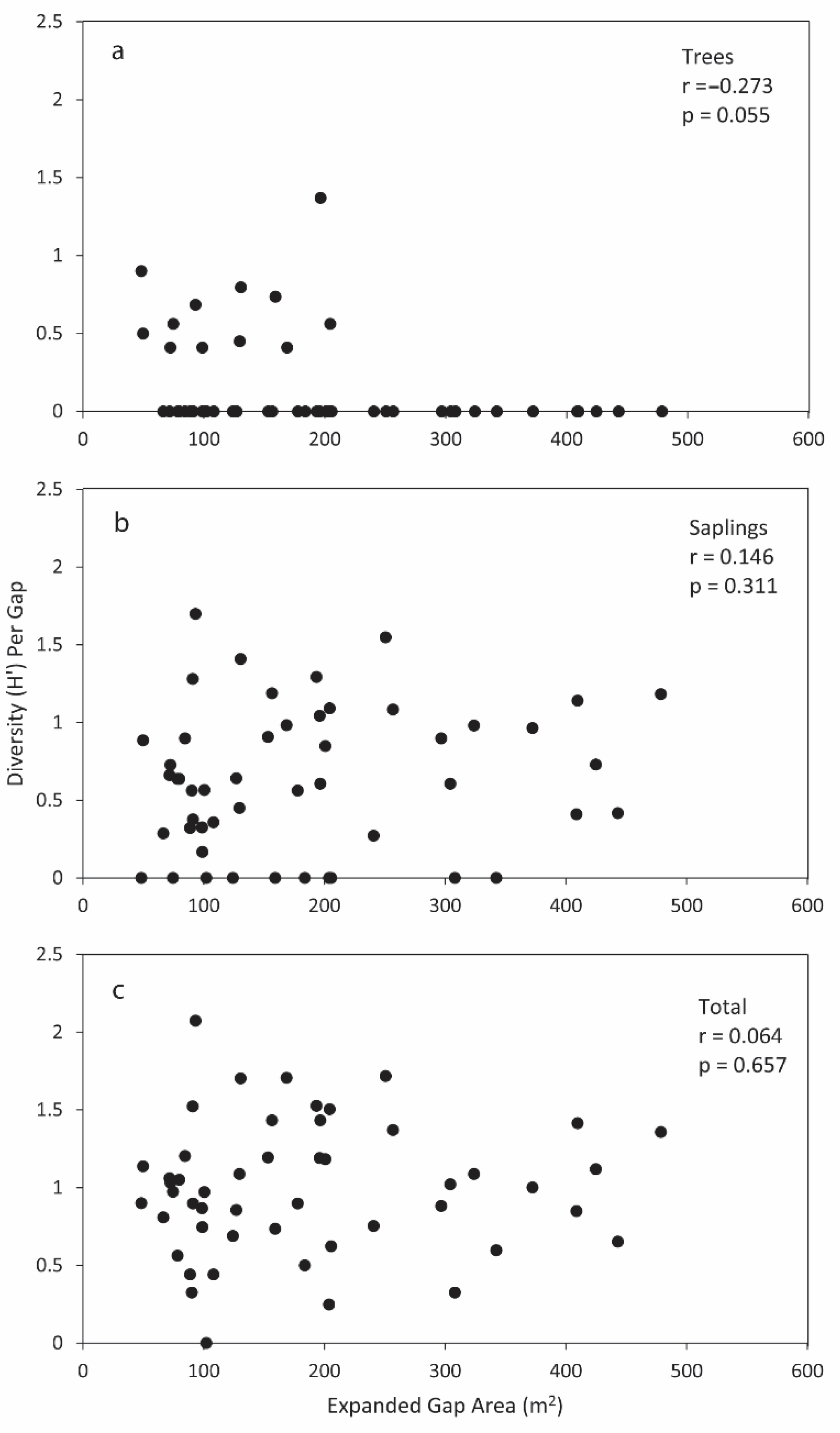
Shannon diversity of the tree layer for canopy gap plots 0.39 and for reference plots was 0.31. No significant relationship existed between expanded gap area and tree-layer Shannon diversity (r = −0.273, p = 0.055; Figure 3). Sapling-layer Shannon diversity was 1.50 in canopy gap plots and 1.38 in reference plots. No significant relationship occurred between expanded gap area and sapling-layer Shannon diversity (r = 0.146, p = 0.311). Likewise, we found no significant relationship between expanded gap area and Shannon diversity of the tree and sapling layers combined (r = 0.064, p = 0.657). Shannon diversity of the seedling layer in canopy gap plots was 1.26 and was 1.37 in reference plots.

3.3. Gap Closure Mechanisms

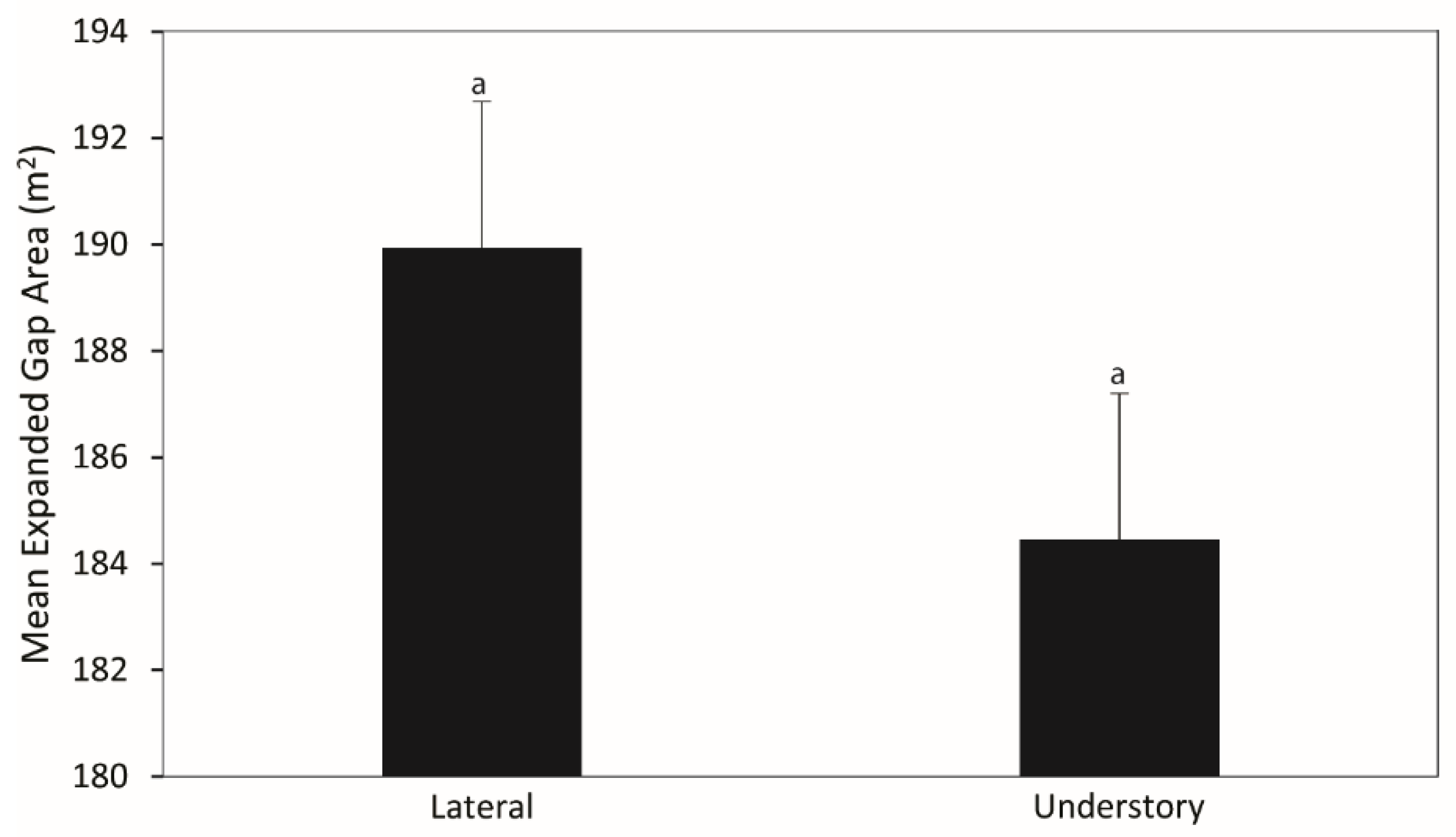
We projected that 74% of the sampled canopy gaps would close through lateral crown expansion and 26% would close through understory capture. Out of the 13 canopy gaps predicted to close through understory capture, eight were projected to be captured by Pinus palustris. We also projected that one canopy gap would be captured by a Liquidambar styraciflua, one by a Pinus taeda, and one by a Quercus stellata. For two canopy gaps projected to close by understory capture, we could not with confidence identify the species of the ascension tree as these gaps had many sub-canopy stems of similar height. Expanded gap area did not significantly differ by canopy gap closure mechanism (p = 0.300; Figure 4). Likewise, we found no significant difference between mean basal area lost by projected gap closure mechanism (p = 0.882). Similarly, a mean expanded gap L:W and D:H ratios did not significantly differ by a canopy gap closure mechanism (p = 0.800 and p = 0.106, respectively).

3.4. Gap Fraction and Spatial Distribution

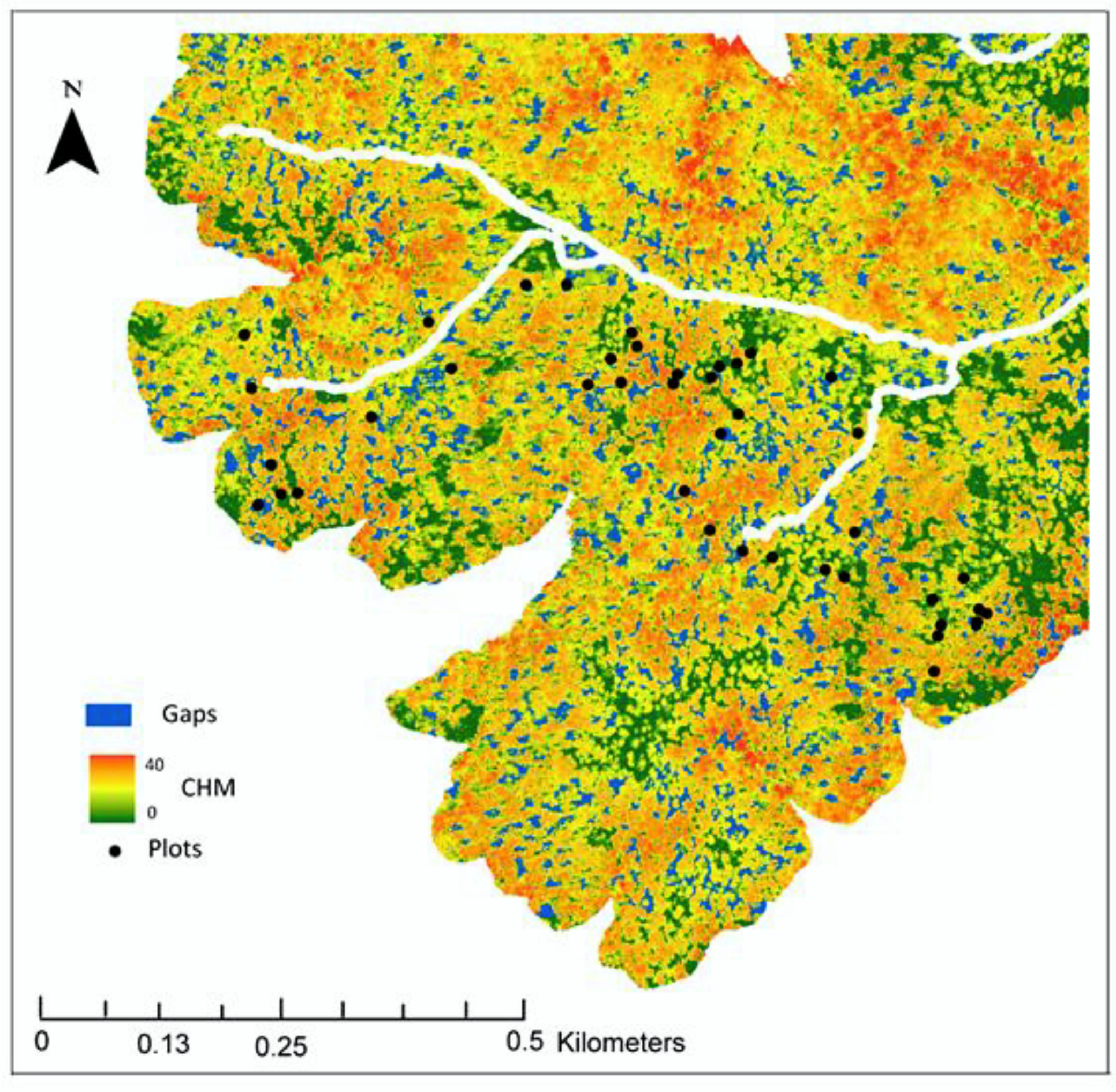
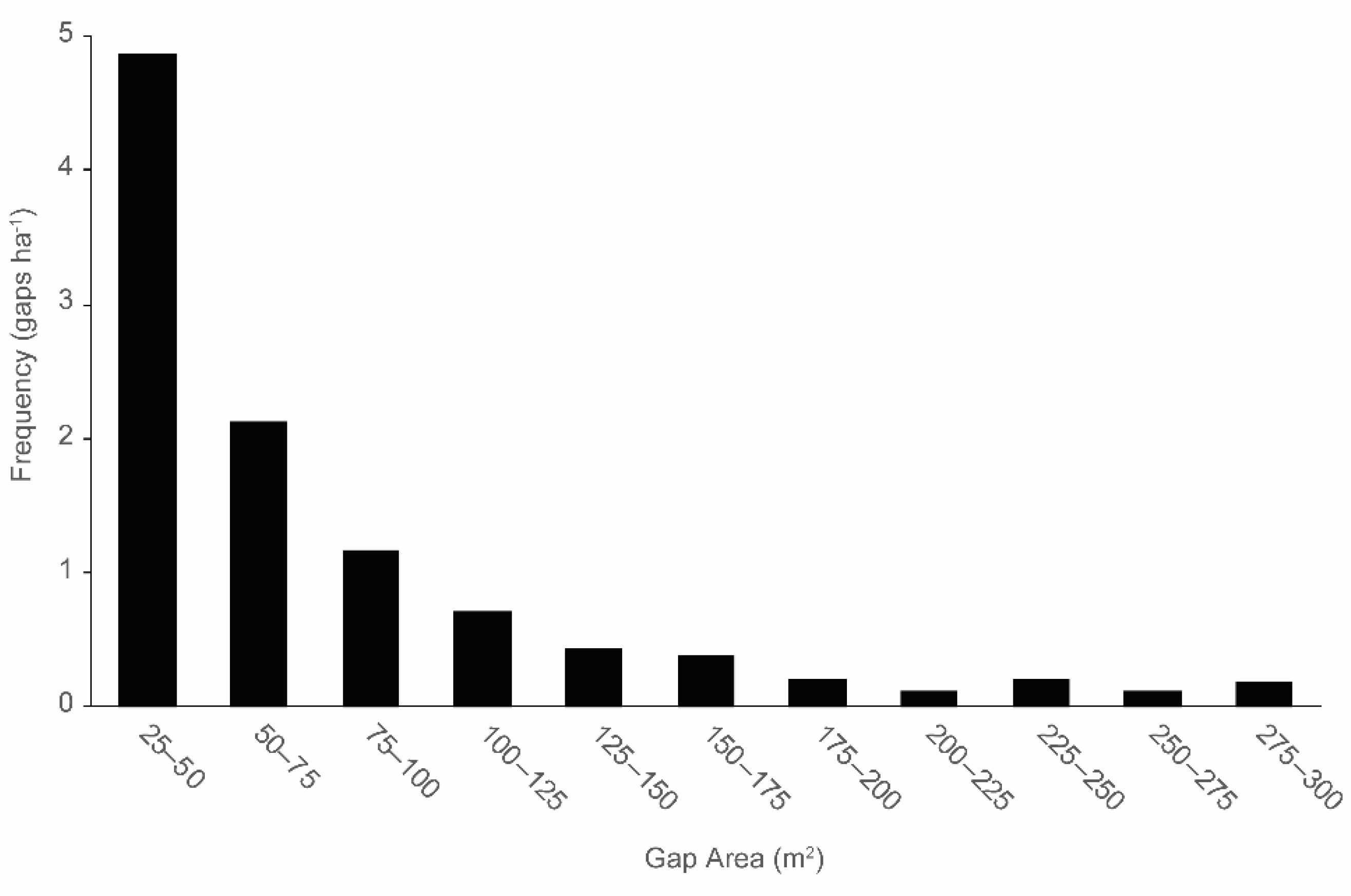
From the canopy height model, we detected a total of 742 observed canopy gaps (11 canopy gaps/ha; Figure 5). The average observed canopy gap area was 76 m2 ± 60, with a minimum area of 25 m2, and a maximum area of 298 m2 (Figure 6). The canopy gap size-frequency distribution exhibited a reverse J-shape, with a high frequency of small-area canopy gaps and relatively few large-area canopy gaps (Figure 6). We detected 2.12 gaps/ha in the 50–75 m2 size bin, 1.17 canopy gaps/ha in the 75–100 m2 area bin, and 0.71 canopy gaps/ha in the 100–125 m2 area bin. Detected canopy gaps exhibited significant spatial dispersion at short distances and significant spatial clustering at greater distances (Figure 7). Specifically, canopy gaps were less likely to be observed at distances of 1–8 m from an adjacent gap (significant dispersion). Canopy gaps were more likely to be observed at distances of 12–36 m from an adjacent gap (significant clustering). At distances > 36 m, detected canopy gaps exhibited random spatial distribution.

4. Discussion

4.1. Canopy Gap and Gapmaker Characteristics

The majority of canopy gaps in this P. palustris woodland were formed by single standing dead trees. In contrast, single-tree gaps caused by uprooted or snapped stems were least common. Compared to the co-occurring Pinus taeda, P. palustris is more susceptible to stem snapping and uprooting when exposed to strong winds [74,75]. Pinus palustris snags have been well studied, and they may result from mortality by lightning, insects, or fire and may be important for wildlife habitat and fire ignition [21,31,54,76,77,78]. In our non-gap reference plots, we found snag density was 5/ha and all but one snag, a Q. falcata, was a P. palustris stem. Landers and Boyer [76] found a snag density of 7/ha and Varner et al. [19] reported snag density of 9–11/ha for complex stage P. palustris stands. When canopy gap areas are included, snag density for this montane, P. palustris woodland approximated the snag density reported in other P. palustris stands, including those stands in late stages of stand development.
We posit that many of the snag-formed canopy gaps we documented were caused by Dendroctonus frontalis Zimm. activity. In fact, out of 50 plots, 20 showed beetle activity on gapmakers, and 13 of those 20 canopy gaps were formed fully or partially by snags. We found canopy gaps created by gapmakers with evidence of beetle activity formed in 2004, 2005, 2010, 2011, 2012, 2014, 2016, 2018, and 2019. We suspect that insect-induced mortality is an important gap formation mechanism in P. palustris woodlands. Attached trees that succumb would become snags that may eventually snap during strong wind events. In contrast, we suspect that strong winds, especially those associated with intense precipitation, may result in relatively more uprooting of living stems [45].
Unexpectedly, multi-tree canopy gaps had marginally smaller mean observed and expanded gap areas than single tree canopy gaps. Although the differences were not significant, the finding was surprising. We suggest this might be related to the size of the trees removed during gap formation. Gapmakers in single tree canopy gaps were significantly larger than gapmakers in multi-tree canopy gaps. Tree diameter is related to crown volume and thus some of the single tree-formed gaps were caused by mortality of relatively large trees that represented accordingly large canopy areas. In contrast, gapmakers in some multi-tree gaps were relatively small and therefore constituted a smaller portion of the forest canopy. Runkle [79] found gapmakers to be larger than surrounding trees; however, other gap-scale disturbance studies have not found this pattern [56,57].
Canopy gap ages ranged from over 20 years to 1 year in our study. Out of 50 canopy gaps sampled, seven gaps had unknown ages, as there was no agreement on the formation year between multiple samples taken for those events. Based on the age distribution we documented, we suspect that canopy gaps in this woodland ecosystem may remain open for ca. 20–25 years, but we note that some gaps would close in shorter periods. The average age of canopy gaps was 10 years (gaps formed in 2011), and the most common age was 16 years (gaps formed in 2005). If canopy gaps are being formed at the approximate rate that canopy gaps are closing, then gap fraction is considered to be in dynamic equilibrium [80]. In such instances, we would expect a high number of young gaps and the number of canopy openings should decrease with increased gap age [6]. The canopy gap age distribution we observed in this Pinus woodland indicated that gap fraction was not in equilibrium. This is not unusual or unexpected as superimposed over the natural background mortality rate are exogenous disturbance events that may cause the gap age distribution to become irregular [57].
Canopy openings without gapmakers were found while walking transects through the woodland but were not sampled because they did not meet our established canopy gap criteria. This could be an indication of gap-scale disturbance where the gapmaker(s) had decomposed completely, but more likely indicated intermediate-severity disturbance events where canopy openings would have been larger than that of canopy gaps [2]. Intermediate-severity disturbances would impact larger areas than canopy gaps and would therefore take longer periods to close the canopy voids so that the gap remained after the gapmakers had decomposed. We suspect that some of the canopy openings we observed without visible gapmakers were the result of these broader-scale disturbance events.
As suspected, reference plots (i.e., closed canopy locations) had significantly more litter than canopy gaps plots. Overstory density in P. palustris stands has been shown to be a strong predictor of Pinus needle litter [32]. We suspect that open canopy conditions caused by the loss of one or more Pinus canopy trees reduced Pinus litter cover and increased herb cover within canopy gaps [14]. The spatial variability in Pinus litter and herb cover may influence fire behavior such that reference plots, with higher fuel loads, would have different fire effects than canopy gap microenvironments [31,81].
L:W ratios can be used to quantify canopy gap shapes and may provide information on micro-scale variations that occur within individual gap types [56]. We found no significant difference between L:W and a gap formation mechanism. Snag-formed gaps have been shown to be more circular in shape than those caused by uprooted stems which may be more elliptical [56]; however, not all studies have documented relationships between L:W and gap formation mechanism [57]. Canopy closure mechanisms could also be influenced by L:W, as gap L:W may influence insolation in the sub-canopy [82,83]. The shape of the gaps may also influence gap closure as narrow gaps would be more likely to fill by lateral branch extension; however, we noted no relationships between gap closure mechanism and L:W. Similarly, we found no significant relationship between D:H and canopy closure mechanism.

4.2. Forest Composition

Shannon diversity was significantly greater in canopy gap plots than in reference plots for both seedling and sapling sized stems. Higher species diversity within canopy gap plots was not surprising and was likely a function of the increased resources associated with those microenvironments [14,16,22,53]. Hardwood saplings were more abundant than P. palustris or other Pinus species saplings in both canopy gap and reference plots. Pecot et al. [20] found that hardwood advance reproduction in P. palustris canopy gaps had the advantage of established root systems that allowed for faster vertical growth rates. However, with recurring surface fires, hardwood individuals should disproportionately be maintained in the seedling and sapling size categories as stems should continually be top killed [26,84]. Shoot mortality can vary depending, in part, on species and stem size (which can impact bark thickness and bud height) and fire behavior (which can influence the temperatures to which stems are exposed). Shannon diversity of trees, saplings, and total trees and saplings were not significantly correlated with expanded canopy gap area. This indicated that larger canopy gaps do not have higher Shannon diversity values than smaller canopy gaps, but regardless, canopy gap environments do support greater woody plant diversity than non-gap microenvironments.

4.3. Gap Closure Mechanisms

The majority of canopy gaps were projected to close through lateral crown extension. Pinus palustris was the species most likely to capture canopy gaps through lateral extension, or from subcanopy height growth. Few canopy gaps were predicted to be captured by a species other than P. palustris, despite relatively high species richness in the regeneration layer. The other species projected to capture canopy gaps from below were Liquidambar styraciflua, Quercus stellata, and P. taeda. Notably, the gaps projected to be captured by a Quercus or a P. taeda contained canopy gap perimeter trees of the same species. The canopy of the woodland was almost purely P. palustris, so these microsites that contained canopy trees of other species may have had some underlying conditions that favored those species over P. palustris. Nonetheless, most all canopy gaps were projected to be closed via P. palustris. Thus, under the current disturbance regime, we suggest that P. palustris will remain the dominant species throughout the fire-maintained woodland. Recurring low intensity fires disproportionately kill shoots of fire-sensitive species thereby reducing competition for P. palustris recruitment via gap-scale processes [21,30,85].
We suspected that smaller canopy gaps would be more likely to close through lateral crown extension and larger canopy gaps would be more likely to close through understory capture [57,86]. However, the canopy gap closure mechanism was not impacted by expanded gap area or basal area lost via gap formation. In fact, both the largest and smallest canopy gaps were predicted to close through understory capture. This indicated that factors other than expanded canopy gap area and basal area removed by gap formation influence the gap closure mechanism. Lertzman [87] found that gap closure mechanisms were reliant on the presence of advance reproduction in the canopy gap environment and noted that species most abundant in the understory were most likely to fill the canopy void.

4.4. Gap Fraction and Spatial Distribution

Our use of LiDAR to calculate gap fraction removed potential bias that may result from sampling only canopy gaps found along established transects in the field [52]. Observed canopy gap areas for the sampled gaps and the LiDAR detected gaps were similar (mean area of the observed canopy gaps in the field was 75 m2 and mean area of LiDAR-detected gaps was 76 m2). In general, the canopy gaps documented in this montane P. palustris woodland were smaller than typical sizes observed in P. palustris stands on the Coastal Plain [22]. Our analysis did reveal some canopy openings larger than 300 m2 (the threshold set in our analysis). These large openings indicated the presence of intermediate-severity disturbance events through the P. palustris woodland [2]. The gap-size frequency distribution exhibited a reverse-J or negative exponential shape. Although we set a maximum gap area threshold of 300 m2, we speculated that the frequency of large openings would be less than that of small gaps, as has been reported in many canopy gap-based studies in a variety of forest types and among a variety of disturbance agents (e.g., [88,89,90]).
The forest-scale spatial distribution of detected canopy gaps exhibited a significantly dispersed pattern (i.e., distance between gaps greater than expected under CSR) at short distances and a significantly clustered pattern (i.e., distance between gaps less than expected under CSR) at distances up to 36 m. The significant dispersion at distances <8 m was likely attributed to P. palutris individuals that occurred between single-tree gaps. We expect the crown diameter of canopy P. palutris to approximate the distances at which significant dispersion of canopy gaps occurred [91]. At distances of 8–36 m, canopy gaps were clustered in space. The significant clustering of canopy gaps at intermediate distances could be attributed to Dendroctonus frontalis activity, localized drought stress, patchy high severity fire, or other exogenous canopy disturbance in which trees in small neighborhoods experienced the same discreet disturbance. Our findings correspond to spatial patterns reported in other canopy gap studies that found both clustered and dispersed patterns of canopy gaps depending on distance. Canopy gaps that result from insects, pests, pathogens or endogenous disturbance have been found to be evenly dispersed or randomly distributed [92,93,94], which we documented at distances >36 m. Clustered patterns have been associated with exogenous disturbance such as wind, or other gap-enlarging agents, but these patterns manifested at greater distances than what we documented in this study [94,95]. We suspect we may have found significant clustering of canopy gaps at greater distances if large openings (those > 300 m2) were included in our spatial analyses.

5. Conclusions

Although gap-scale disturbances are the most common disturbance events in forest ecosystems, few studies have analyzed gap-scale disturbance patterns and processes in Pinus palustris woodlands. Most canopy gaps (64%) we documented were caused by the death of a single tree, but multi-tree gaps were not uncommon. Snag-formed gaps were most frequent (38%) followed by snapped stem-formed gaps (32%). We speculated that many canopy gaps were caused by insects. Furthermore, we suspected that gap formation may be higher during periods of water stress, but additional research is required. Contrary to our expectations, we did not find significant differences in gap size or shape patterns based on gap formation or closure mechanisms. Most gaps (74%) were projected to close by lateral crown expansion of gap perimeter trees. Through this process, canopy trees, which were almost exclusively P. palustris, would increase crown area. We hypothesized that most gaps projected to close via subcanopy recruitment would be captured by a P. palustris stem, but we did note a canopy gap projected to close by a P. taeda, one projected to close by a Q. stellata, and one projected to close by a L. styraciflua individual. Pinus litter was the most common ground cover in both canopy gap and non-gap environments, but litter depth was significantly greater in non-gap plots. The majority of gaps were small and gap frequency declined with increased gap size. We found gaps were significantly clustered at distances of 8–36 m from gap edge to gap edge, but were randomly distributed beyond 36 m. With frequent prescribed fire, we hypothesized that gap-scale disturbance processes would maintain P. palustris dominance in this woodland and that, through these processes, stand structure would transition to a lower density of larger canopy trees at wider spacings. As stand structure changes over time, gap-scale disturbance patterns and processes may change accordingly.

Author Contributions

Conceptualization, H.L.M. and J.L.H.; methodology, H.L.M., J.D.G., and J.L.H.; formal analysis, H.L.M. and J.D.G.; writing—original draft preparation, H.L.M.; writing—review and editing, J.D.G. and J.L.H.; All authors have read and agreed to the published version of the manuscript.

Funding

This research received no external funding.

Institutional Review Board Statement

Not applicable.

Informed Consent Statement

Not applicable.

Data Availability Statement

Data are available from the corresponding author upon reasonable request.

Acknowledgments

We thank the USDA Forest Service, Talladega National Forest, Oakmulgee Ranger District for logistical support and David Phillips and Samantha Luitjens for assistance with field data collection and Brady Allen and John Kiep laboratory assistance.

Conflicts of Interest

The authors declare no conflict of interest.

References

  1. Oliver, C.D.; Larson, B.C. Forest Stand Dynamics; John Wiley and Sons: Hoboken, NJ, USA, 1996. [Google Scholar]
  2. Hart, J.L.; Kleinman, J.S. What are intermediate-severity forest disturbances and why are they important? Forests 2018, 9, 579. [Google Scholar] [CrossRef] [Green Version]
  3. Runkle, J.R. Disturbance regimes in temperate forests. In The Ecology of Natural Disturbance and Patch Dynamics; Pickett, S.T.A., White, P.S., Eds.; Academic Press: San Diego, CA, USA, 1985; pp. 17–33. [Google Scholar]
  4. Yamamoto, S.I. Forest gap dynamics and tree regeneration. J. For. Res. 2000, 5, 223–229. [Google Scholar] [CrossRef]
  5. Frelich, L.E. Forest Dynamics and Disturbance Regimes: Studies from Temperate Evergreen-Deciduous Forests; Cambridge University Press: Cambridge, UK, 2002. [Google Scholar]
  6. Hart, J.L. Gap-scale disturbances in central hardwood forests with implications for management. In Natural Disturbances and Historic Range of Variation; Greenberg, C.H., Collins, B.S., Eds.; Springer: New York, NY, USA, 2016; pp. 33–47. [Google Scholar]
  7. Brokaw, N.V. Gap-phase regeneration in a tropical forest. Ecology 1985, 66, 682–687. [Google Scholar] [CrossRef]
  8. Abe, S.; Masaki, T.; Nakashizuka, T. Factors influencing sapling composition in canopy gaps of a temperate deciduous forest. J. Veg. Sci. 1995, 120, 21–32. [Google Scholar] [CrossRef]
  9. Brokaw, N.; Busing, R.T. Niche versus chance and tree diversity in forest gaps. Trends. Ecol. Evol. 2000, 15, 183–188. [Google Scholar] [CrossRef]
  10. Hart, J.L.; Kupfer, J.A. Sapling richness and composition in canopy gaps of a southern Appalachian mixed Quercus forest. J. Torrey. Bot. Soc. 2011, 138, 207–219. [Google Scholar] [CrossRef]
  11. Canham, C.D.; Marks, P.L. The response of woody plants to disturbance patterns of establishment and growth. In The Ecology of Natural Disturbance and Patch Dynamics; Pickett, S.T.A., White, P.S., Eds.; Academic Press: San Diego, CA, USA, 1985; pp. 197–216. [Google Scholar]
  12. Putz, F.E. Treefall pits and mounds, buried seeds, and the importance of soil disturbance to pioneer trees on Barro Colorado Island, Panama. Ecology 1983, 64, 1069–1074. [Google Scholar] [CrossRef]
  13. Denslow, J.S. Tropical rainforest gaps and tree species diversity. Annu. Rev. Ecol. Evol. Syst. 1987, 18, 431–451. [Google Scholar] [CrossRef]
  14. McGuire, J.P.; Mitchell, R.J.; Moser, E.B.; Pecot, S.D.; Gjerstad, D.H.; Hedman, C.W. Gaps in a gappy forest: Plant resources, longleaf pine regeneration, and understory response to tree removal in longleaf pine savannas. Can. J. For. Res. 2001, 31, 765–778. [Google Scholar] [CrossRef]
  15. Dey, D.C.; Kabrick, J.M. Restoration of midwestern oak woodlands and savannas. In Restoration of Boreal and Temperate Forests, 2nd ed.; Stanturf, J.A., Ed.; CRC Press: Boca Raton, FL, USA, 2015; pp. 401–428. [Google Scholar]
  16. Palik, B.J.; Mitchell, R.J.; Houseal, G.; Pederson, N. Effects of canopy structure on resource availability and seedling responses in a longleaf pine ecosystem. Can. J. For. Res. 1997, 27, 1458–1464. [Google Scholar] [CrossRef]
  17. Battaglia, M.A.; Mitchell, R.J.; Mou, P.P.; Pecot, S.D. Light transmittance estimates in a longleaf pine woodland. For. Sci. 2003, 49, 752–762. [Google Scholar]
  18. Gagnon, J.L.; Jokela, E.J.; Moser, W.K.; Huber, D.A. Dynamics of artificial regeneration in gaps within a longleaf pine flatwoods ecosystem. For. Ecol. Manag. 2003, 172, 133–144. [Google Scholar] [CrossRef]
  19. Varner, J.M., III; Kush, J.S.; Meldahl, R.S. Structural characteristics of frequently-burned old-growth longleaf pine stands in the mountains of Alabama. Castanea 2003, 68, 211–221. [Google Scholar]
  20. Pecot, S.D.; Mitchell, R.J.; Palik, B.J.; Moser, E.B.; Hiers, J.K. Competitive responses of seedlings and understory plants in longleaf pine woodlands: Separating canopy influences above and below ground. Can. J. For. Res. 2007, 37, 634–648. [Google Scholar] [CrossRef]
  21. Platt, W.J.; Evans, G.W.; Rathbun, S.L. The population dynamics of a long-lived conifer (Pinus palustris). Am. Nat. 1988, 131, 491–525. [Google Scholar] [CrossRef]
  22. Brockway, D.G.; Outcalt, K.W. Gap-phase regeneration in longleaf pine wiregrass ecosystems. For. Ecol. Manag. 1998, 106, 125–139. [Google Scholar] [CrossRef]
  23. Gagnon, J.L.; Jokela, E.J.; Moser, W.K.; Huber, D.A. Characteristics of gaps and natural regeneration in mature longleaf pine flatwoods ecosystems. For. Ecol. Manag. 2004, 187, 373–380. [Google Scholar] [CrossRef]
  24. Jack, S.B.; Pecot, S.D. Regeneration Dynamics, Competition, and Seedling Response. In Ecological Restoration and Management of Longleaf Pine Forests; Kirkman, L.K., Jack, S.B., Eds.; CRC Press, Taylor and Francis Group: Boca Raton, FL, USA, 2018; pp. 311–338. [Google Scholar]
  25. Wahlenberg, W.G. Longleaf Pine: Its Use, Ecology, Regeneration, Protection, Growth, and Management; United States Department of Agriculture, Forest Service: Washington, DC, USA, 1946. [Google Scholar]
  26. Boyer, W.D. Natural Regeneration of Longleaf Pine; United States Department of Agriculture, Forest Service, Technical Publication SA-TP3: Washington, DC, USA, 1979. [Google Scholar]
  27. Glitzenstein, J.S.; Streng, D.R.; Wade, D.D. Fire frequency effects on longleaf pine (Pinus palustris P. Miller) vegetation in South Carolina and northeast Florida, USA. Nat. Area. J. 2003, 23, 22–37. [Google Scholar]
  28. Brockway, D.G. Restoration of Longleaf Pine Ecosystems; United States Department of Agriculture, Forest Service, Southern Research Station: Asheville, NC, USA, 2005; Volume 83. [Google Scholar]
  29. Kleinman, J.S.; Hart, J.L. Vascular flora of longleaf pine woodlands after wind disturbance and salvage harvesting in the Alabama Fall Line Hills. Castanea 2018, 83, 183–195. [Google Scholar] [CrossRef]
  30. Jin, S.; Moule, B.; Yu, D.; Wang, G.G. Fire survival of longleaf pine (Pinus palustris) grass stage seedlings: The role of seedling size, root collar position, and resprouting. Forests 2019, 10, 1070. [Google Scholar] [CrossRef] [Green Version]
  31. Mitchell, R.J.; Hiers, J.K.; O’Brien, J.; Starr, G. Ecological forestry in the Southeast: Understanding the ecology of fuels. J. For. 2009, 107, 391–397. [Google Scholar]
  32. Dell, J.E.; Richards, L.A.; O’Brien, J.J.; Loudermilk, E.L.; Hudak, A.T.; Pokswinski, S.M.; Dyer, L.A. Overstory-derived surface fuels mediate plant species diversity in frequently burned longleaf pine forests. Ecosphere 2017, 8, e01964. [Google Scholar] [CrossRef]
  33. Mitchell, R.J.; Hiers, J.K.; O’Brien, J.J.; Jack, S.B.; Engstrom, R.T. Silviculture that sustains: The nexus between silviculture, frequent prescribed fire, and conservation of biodiversity in longleaf pine forests of the southeastern United States. Can. J. For. Res. 2006, 36, 2724–2736. [Google Scholar] [CrossRef] [Green Version]
  34. Mugnani, M.P.; Robertson, K.M.; Miller, D.L.; Platt, W.J. Longleaf pine patch dynamics influence ground-layer vegetation in old-growth pine savanna. Forests 2019, 10, 389. [Google Scholar] [CrossRef] [Green Version]
  35. Beckett, S.; Golden, M.S. Forest vegetation and vascular flora of reed brake research natural area, Alabama. Castanea 1982, 47, 368–392. [Google Scholar]
  36. Hammond, D.H.; Varner, J.M.; Kush, J.S.; Fan, Z. Contrasting sapling bark allocation of five southeastern USA hardwood tree species in a fire prone ecosystem. Ecosphere 2015, 6, 1–13. [Google Scholar] [CrossRef] [Green Version]
  37. Klaus, N.A.; Rush, S.A.; Weitzel, S.L.; Holdrege, M.C. Changes in tree canopy, groundcover, and avian community following restoration of a Montane longleaf pine woodland. Am. Midl. Nat. 2020, 184, 163–176. [Google Scholar] [CrossRef]
  38. Hammond, D.H.; Varner, J.M.; Fan, Z.; Kush, J.S. Long-term stand dynamics of old-growth mountain longleaf pine (Pinus palustris) woodlands. For. Ecol. Manag. 2016, 364, 154–164. [Google Scholar] [CrossRef]
  39. Kressuk, J.M.; Goode, J.D.; Bhuta, A.A.; Hart, J.L.; Kleinman, J.S.; Phillips, D.L.; Willson, K.G. Composition and structure of a montane longleaf pine stand on the Alabama piedmont. Southeast. Nat. 2020, 19, 436–446. [Google Scholar] [CrossRef]
  40. US Department of Agriculture, Forest Service. Longleaf Ecosystem-Restoration Project: Final Environmental Impact Statement, National Forests in Alabama; Talladega National Forest, Oakmulgee District, USDA Forest Service: Brent, AL, USA, 2005; p. 15. [Google Scholar]
  41. Boyer, W.D.; Bledsoe, B.W. Establishment Report: Reed Brake Research Natural Area, National Forests in Alabama, Bibb County, Alabama; United States Department of Agriculture, Forest Service, Southern Forest Experiment Station: Asheville, NC, USA, 1975. [Google Scholar]
  42. Shankman, D.; Hart, J.L. The Fall Line: A Physiographic-Forest Vegetation Boundary. Geogr. Rev. 2007, 97, 502–519. [Google Scholar] [CrossRef]
  43. Cox, L.E.; Hart, J.L. Two centuries of forest compositional and structural changes in the Alabama Fall Line Hills. Am. Midl. Nat. 2015, 174, 218–237. [Google Scholar] [CrossRef]
  44. Kleinman, J.S.; Hart, J.L. Response by vertical strata to catastrophic wind in restored Pinus palustris stands. J. Torrey Bot. Soc. 2017, 144, 423–438. [Google Scholar] [CrossRef]
  45. Kleinman, J.S.; Ford, S.A.; Hart, J.L. Catastrophic wind and salvage harvesting effects on woodland plants. For. Ecol. Manag. 2017, 403, 112–125. [Google Scholar] [CrossRef]
  46. Harper, R.M. Forests of Alabama; Geological Survey of Alabama, Monograph 10; Wetumpka Printing Company: Wetumpka, AL, USA, 1943. [Google Scholar]
  47. Thornthwaite, C.W. An approach toward a rational classification of climate. Geogr. Rev. 1948, 38, 55–94. [Google Scholar] [CrossRef]
  48. PRISM Climate Group. Northwest Alliance for Computational Science and Engineering. Available online: http://www.prism.oregonstate.edu/ (accessed on 1 February 2022).
  49. USDA NRCS (United States Department of Agriculture, Natural Resources Conservation Service). Web Soil Survey. Available online: https://websoilsurvey.nrcs.usda.gov/ (accessed on 1 March 2022).
  50. Anderson, E.W. A guide for estimating cover. Rangelands 1986, 8, 236–238. [Google Scholar]
  51. Kleinman, J.S.; Goode, J.D.; Hart, J.L.; Dey, D.C. Prescribed fire effects on Pinus palustris woodland development after catastrophic wind disturbance and salvage logging. For. Ecol. Manag. 2020, 468, 118173. [Google Scholar] [CrossRef]
  52. Runkle, J.R. Guidelines and Sample Protocol for Sampling Forest Gaps; United States Department of Agriculture, Forest Service, Pacific Northwest Research Station: Asheville, NC, USA, 1992; Volume 283. [Google Scholar]
  53. Runkle, J.R. Patterns of disturbance in some old-growth mesic forests of eastern North America. Ecology 1982, 63, 1533–1546. [Google Scholar] [CrossRef] [Green Version]
  54. Ulyshen, M.D.; Horn, S.; Pokswinski, S.; McHugh, J.V.; Hiers, J.K. A comparison of coarse woody debris volume and variety between old-growth and secondary longleaf pine forests in the southeastern United States. For. Ecol. Manag. 2018, 429, 124–132. [Google Scholar] [CrossRef]
  55. Taylor, S.O.; Lorimer, C.G. Loss of oak dominance in dry-mesic deciduous forests predicted by gap capture methods. J. Plant. Ecol. 2003, 167, 71–88. [Google Scholar] [CrossRef]
  56. Hart, J.L.; Grissino-Mayer, H.D. Gap-scale disturbance processes in secondary hardwood stands on the Cumberland Plateau, Tennessee, USA. J. Plant. Ecol. 2009, 201, 131–146. [Google Scholar] [CrossRef]
  57. Richards, J.D.; Hart, J.L. Canopy gap dynamics and development patterns in secondary Quercus stands on the Cumberland Plateau, Alabama, USA. For. Ecol. Manag. 2011, 262, 2229–2239. [Google Scholar] [CrossRef]
  58. Weber, T.A.; Hart, J.L.; Schweitzer, C.J.; Dey, D.C. Influence of gap-scale disturbance on developmental and successional pathways in Quercus-Pinus stands. For. Ecol. Manag. 2014, 331, 60–70. [Google Scholar] [CrossRef]
  59. Barden, L.S. Tree replacement in small canopy gaps of a Tsuga canadensis forest in the southern Appalachians, Tennessee. Oecologia 1979, 44, 141–142. [Google Scholar] [CrossRef]
  60. Barden, L.S. Tree replacement in a cove hardwood forest of the southern Appalachians. Oikos 1980, 35, 16–19. [Google Scholar] [CrossRef]
  61. White, P.S.; MacKenzie, M.D.; Busing, R.T. Natural disturbance and gap-phase dynamics in southern Appalachian spruce-fir forests. Can. J. For. Res. 1985, 15, 233–240. [Google Scholar] [CrossRef]
  62. Yamamoto, S.; Nishimura, N. Canopy gap formation and replacement pattern of major tree species among developmental stages of beech (Fagus crenata) stands, Japan. J. Plant. Ecol. 1999, 140, 167–176. [Google Scholar] [CrossRef]
  63. Stokes, M.A.; Smiley, T.L. An Introduction to Tree-Ring Dating; University of Arizona Press: Tucson, AZ, USA, 1996. [Google Scholar]
  64. Villalba, R.; Veblen, T.T. Improving estimates of total tree ages based on increment core samples. Ecoscience 1997, 4, 534–542. [Google Scholar] [CrossRef]
  65. Rubino, D.L.; McCarthyz, B.C. Comparative analysis of dendroecological methods used to assess disturbance events. Dendrochronologia 2004, 21, 97–115. [Google Scholar] [CrossRef]
  66. Hart, J.L.; van de Gevel, S.L.; Grissino-Mayer, H.D. Forest dynamics in a natural area of the southern Ridge and Valley, Tennessee. Nat. Areas J. 2008, 28, 275–289. [Google Scholar] [CrossRef] [Green Version]
  67. Beland, M.; Parker, G.; Sparrow, B.; Harding, D.; Chasmer, L.; Phinn, S.; Antonarakis, A.; Strahler, A. On promoting the use of lidar systems in forest ecosystem research. For. Ecol. Manag. 2019, 450, 117484. [Google Scholar] [CrossRef]
  68. NEON (National Ecological Observatory Network). Elevation-LiDAR, Release-2022 (DP3.30024.001). Available online: https://data.neonscience.org/data-products/DP3.30024.001 (accessed on 15 November 2021).
  69. NEON. Data Product. Available online: https://data.neonscience.org/data-products/explore (accessed on 15 November 2021).
  70. Silva, C.A.; Valbuena, R.; Pinagé, E.R.; Mohan, M.; de Almeida, D.R.; Broadbent, E.; Jaafar, W.S.W.M.; Papa, D.A.; Cardil, A.; Klauberg, C. ForestGapR: An r Package for forest gap analysis from canopy height models. Methods. Ecol. Evol. 2019, 10, 1347–1356. [Google Scholar] [CrossRef] [Green Version]
  71. Koukoulas, S.; Blackburn, G.A. Quantifying the spatial properties of forest canopy gaps using LiDAR imagery and GIS. Int. J. Remote. Sens. 2004, 25, 3049–3072. [Google Scholar] [CrossRef]
  72. Wiegand, T.; Kissling, W.D.; Cipriotti, P.A.; Aguiar, M.R. Extending point pattern analysis for objects of finite size and irregular shape. J. Ecol. 2006, 94, 825–837. [Google Scholar] [CrossRef]
  73. Wiegand, T.; Moloney, K.A. Handbook of Spatial Point Pattern Analysis in Ecology; Chapman and Hall/CRC Press: Boca Raton, FL, USA, 2014. [Google Scholar]
  74. Rutledge, B.T.; Cannon, J.B.; McIntyre, R.K.; Holland, A.M.; Jack, S.B. Tree, stand, and landscape factors contributing to hurricane damage in a Coastal Plain forest: Post-hurricane assessment in a longleaf pine landscape. For. Ecol. Manag. 2021, 481, 118724. [Google Scholar] [CrossRef]
  75. Johnsen, K.H.; Butnor, J.R.; Kush, J.S.; Schmidtling, R.C.; Nelson, C.D. Hurricane Katrina winds damaged longleaf pine less than loblolly pine. South. J. Appl. For. 2009, 33, 178–181. [Google Scholar] [CrossRef] [Green Version]
  76. Landers, J.L.; Boyer, W.D. An Old-Growth Definition for Upland Longleaf and South Florida Slash Pine forests, Woodlands, and Savannas; United States Department of Agriculture, Forest Service, Southern Research Station: Asheville, NC, USA, 1999; Volume 29. [Google Scholar]
  77. Blanc, L.A.; Walters, J.R. Cavity-nesting community webs as predictive tools: Where do we go from here? J. Ornithol. 2007, 148, 417–423. [Google Scholar] [CrossRef]
  78. Outcalt, K.W. Lightning, fire and longleaf pine: Using natural disturbance to guide management. For. Ecol. Manag. 2008, 255, 3351–3359. [Google Scholar] [CrossRef] [Green Version]
  79. Runkle, J.R. Changes in southern Appalachian canopy tree gaps sampled thrice. Ecology 1998, 79, 1768–1780. [Google Scholar] [CrossRef]
  80. Himes, J.M.; Rentch, J.S. Canopy gap dynamics in a second-growth Appalachian hardwood forest in West Virginia. Castanea 2013, 78, 171–184. [Google Scholar] [CrossRef]
  81. Emery, R.K.; Kleinman, J.S.; Goode, J.D.; Hart, J.L. Effects of catastrophic wind disturbance, salvage logging, and prescribed fire on fuel loading and composition in a Pinus palustris woodland. For. Ecol. Manag. 2020, 478, 118515. [Google Scholar] [CrossRef]
  82. Canham, C.D. Suppression and release during canopy recruitment in Fagus grandifolia. Bull. Torrey Bot. Club. 1990, 117, 1–7. [Google Scholar] [CrossRef]
  83. De Lima, R.A.F.; Prado, P.I.; Martini, A.M.Z.; Fonseca, L.J.; Gandolfi, S.; Rodrigues, R.R. Improving methods in gap ecology: Revisiting size and shape distributions using a model selection approach. J. Veg. Sci. 2013, 24, 484–495. [Google Scholar] [CrossRef]
  84. Bigelow, S.W.; Whelan, A.W. Longleaf pine proximity effects on air temperatures and hardwood top-kill from prescribed fire. Fire. Ecol. 2019, 15, 1–14. [Google Scholar] [CrossRef]
  85. Outcalt, K.W.; Brockway, D.G. Structure and composition changes following restoration treatments of longleaf pine forests on the Gulf Coastal Plain of Alabama. For. Ecol. Manag. 2010, 259, 1615–1623. [Google Scholar] [CrossRef]
  86. Pedersen, B.S.; Howard, J.L. The influence of canopy gaps on overstory tree and forest growth rates in a mature mixed-age, mixed-species forest. For. Ecol. Manag. 2004, 196, 351–366. [Google Scholar] [CrossRef]
  87. Lertzman, K.P. Patterns of gap-phase replacement in a subalpine, old-growth forest. Ecology 1992, 73, 657–669. [Google Scholar] [CrossRef]
  88. Hobi, M.L.; Ginzler, C.; Commarmot, B.; Bugmann, H. Gap pattern of the largest primeval beech forest of Europe revealed by remote sensing. Ecosphere 2015, 6, 1–15. [Google Scholar] [CrossRef] [Green Version]
  89. Feldmann, E.; Drößler, L.; Hauck, M.; Kucbel, S.; Pichler, V.; Leuschner, C. Canopy gap dynamics and tree understory release in a virgin beech forest, Slovakian Carpathians. For. Ecol. Manag. 2018, 415, 38–46. [Google Scholar] [CrossRef]
  90. Goodbody, T.R.; Tompalski, P.; Coops, N.C.; White, J.C.; Wulder, M.A.; Sanelli, M. Uncovering spatial and ecological variability in gap size frequency distributions in the Canadian boreal forest. Sci. Rep. 2020, 10, 1–12. [Google Scholar] [CrossRef] [Green Version]
  91. Phillips, D.L.; Goode, J.D.; Hart, J.L. Spatial patterns of stand structure and canopy disturbance in a fire-maintained Pinus palustris woodland. Appl. Veg. Sci. 2022, 25, e12657. [Google Scholar] [CrossRef]
  92. Woods, K.D. Intermediate disturbance in a late-successional hemlock-northern hardwood forest. J. Ecol. 2004, 92, 464–476. [Google Scholar] [CrossRef]
  93. Worrall, J.J.; Lee, T.D.; Harrington, T.C. Forest dynamics and agents that initiate and expand canopy gaps in PiceaAbies forests of Crawford Notch, New Hampshire, USA. J. Ecol. 2005, 93, 178–190. [Google Scholar] [CrossRef]
  94. Curzon, M.T.; Keeton, W.S. Spatial characteristics of canopy disturbances in riparian old-growth hemlock–northern hardwood forests, Adirondack Mountains, New York, USA. Can. J. For. Res. 2010, 40, 13–25. [Google Scholar] [CrossRef]
  95. Koukoulas, S.; Blackburn, G.A. Spatial relationships between tree species and gap characteristics in broad-leaved deciduous woodland. J. Veg. Sci. 2005, 16, 587–596. [Google Scholar] [CrossRef]
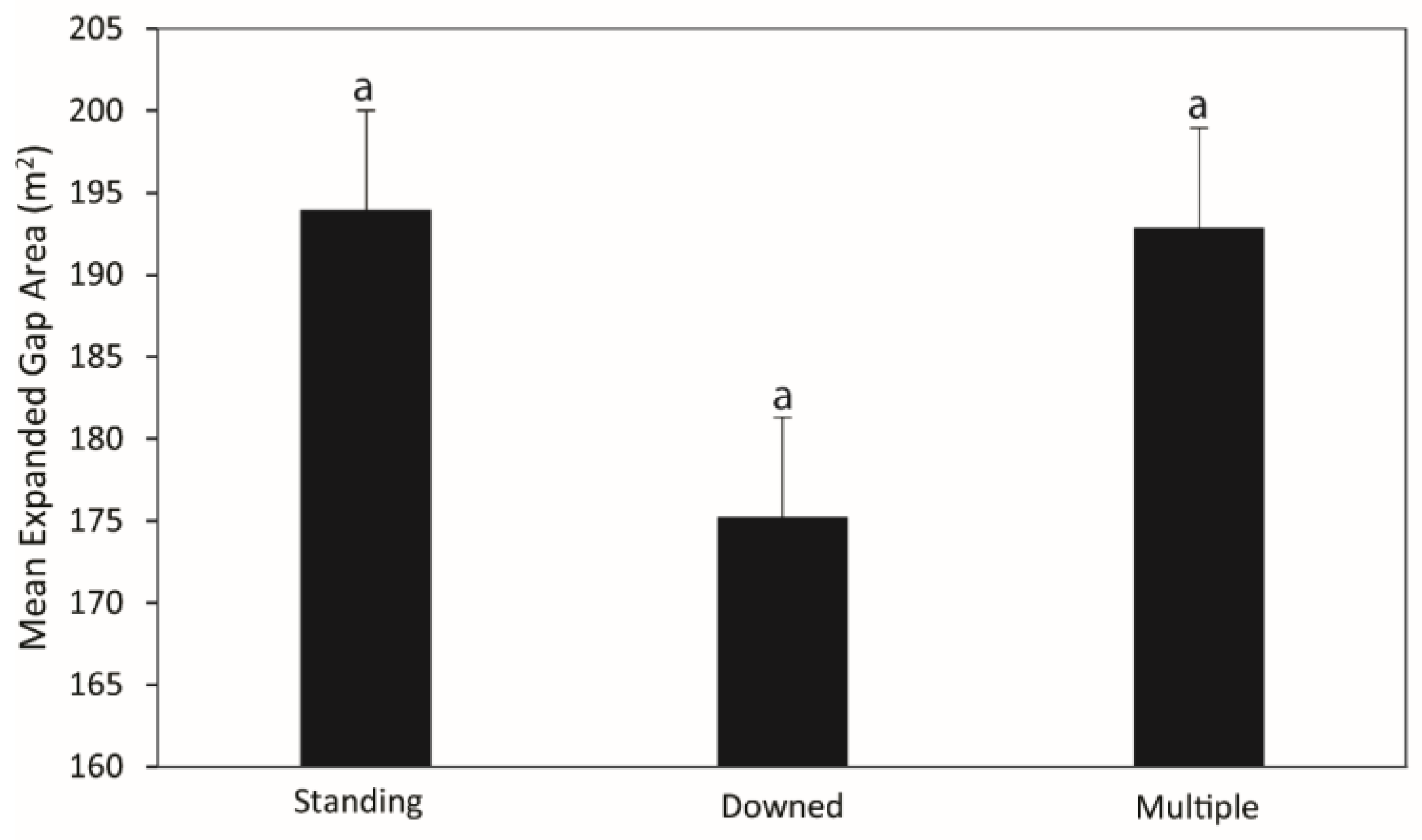
Figure 1. Mean expanded gap area for canopy gaps formed by single standing trees (snags), single downed (snapped and uprooted) trees, and multi-tree gaps in a montane Pinus palustris woodland. Different letters indicate a significant (p < 0.05) difference between categories.
Forests 13 01169 g001
Figure 2. Pearson correlation between expanded gap area and the number of stems for (a) trees (live stems ≥ 10 cm dbh), (b) saplings (live woody stems ≥ 1 m height, <10 cm dbh), and (c) total stems (trees and saplings) in a montane Pinus palustris woodland. Note that the y-axis varies.
Forests 13 01169 g002
Figure 3. Pearson correlation between expanded gap area and Shannon diversity for (a) trees (live stems ≥ 10 cm dbh), (b) saplings (live woody stems ≥ 1 m height, <10 cm dbh), and (c) total stems (trees and saplings) in a montane Pinus palustris woodland.
Forests 13 01169 g003
Figure 4. Mean expanded gap area for canopy gaps projected to close via lateral branch elongation and via understory recruitment in a montane Pinus palustris woodland. Different letters indicate a significant (p < 0.05) difference between categories.
Forests 13 01169 g004
Figure 5. Map of a Pinus palutris dominated stand situated in Reed Brake Research Natural Area, Oakmulgee Ranger District, Talladega National Forest, Alabama, USA. The canopy height model displayed was derived from LiDAR data, with detected canopy gaps in blue. Black dots represent canopy gap sampling plots. Note that our maximum gap size threshold was 300 m2. The white area within the canopy height model is the 10 m buffer around abandoned skid trails.
Forests 13 01169 g005
Figure 6. Gap size-frequency distribution of canopy gaps identified from a LiDAR-derived canopy height model. Canopy gap size bins are 25 m2 size classes. Note our maximum gap size threshold was 300 m2.
Forests 13 01169 g006
Figure 7. Univariate O-ring function O(r) of canopy gaps in a montane Pinus palutris woodland. Point-pattern analysis was adapted for objects with finite size and real shape (i.e., canopy gaps). Shaded areas represent a 95% confidence envelope simulated 99 times under the assumption of complete spatial randomness (CSR). The red line is observed values. Values above the gray shaded area indicate significant (p < 0.05) clustering (i.e., gaps were closer in space than expected when compared to gap locations simulated under the assumption of CSR), and values below the shaded area represent significant dispersion of gaps. Goodness-of-fit (GOF) is reported in the top left.
Forests 13 01169 g007
Table 1. Density, relative density, dominance, relative dominance, and relative importance (average of relative density and relative dominance) for trees (stems ≥ 10 cm dbh) for canopy gap and reference (non-gap) plots in a montane Pinus palustris woodland.
Canopy GapsReference Plots
SpeciesDensity/haRel. den.Dom. (m2/ha)Rel. dom.Rel. imp.Density/haRel. den.Dom. (m2/ha)Rel. dom.Rel. imp.
Pinus palustris Mill. 32.8093.033.6596.0394.53387.0094.6231.9098.1796.39
Quercus falcata Michx. 0.431.210.051.411.311.000.240.010.030.14
Quercus marilandica Münchh. 0.531.520.030.731.123.000.730.090.290.51
Pinus taeda L. 0.431.210.030.740.985.001.220.210.630.93
Quercus stellata Wangenh. 0.431.210.020.420.814.000.980.120.370.67
Carya tomentosa (Lam.) Nutt.0.210.610.000.110.361.000.240.020.080.16
Nyssa sylvatica Marshall.0.210.610.000.050.33 - - - - -
Oxydendrum arboreum (L.) DC. 0.110.300.010.270.292.000.490.020.060.27
Quercus alba L.0.110.300.010.240.27 - - - - -
Quercus laevis Walter - - - - - 4.000.980.030.080.53
Pinus Virginiana Mill. - - - - - 2.000.490.100.300.40
Total 35.251003.8010010040910032.50100100
Table 2. Density and relative density for saplings (stems ≥ 1 m tall, <10 cm dbh) in canopy gap and reference (non-gap) plots in a montane Pinus palustris woodland.
Canopy GapsReference Plots
SpeciesDensity/haRel. den.Density/haRel. den.
Vaccinium arboreum Marshall11959.8182358
Liquidambar styraciflua L. 188.84624.37
Oxydendrum arboreum (L.) DC. 168.330521.49
Symplocos tinctoria (L.) L’Hér.167.92332.33
Rhus copallinum L. 146.9181.27
Diospyros virginiana L. 52.69 - -
Acer rubrum L. 21.24402.82
Pinus palustris Mill. 21.02503.52
Quercus marilandica Münchh. 10.7 - -
Ditrysinia fruticosa (W. Bartram) Govaerts & Frodin10.54 - -
Nyssa sylvatica Marshall.10.48674.72
Vaccinium stamineum L. 10.2730.21
Cornus florida L. 10.2210.07
Quercus falcata Michx. 10.2210.07
Carya tomentosa (Lam.) Nutt.00.16 - -
Quercus laevis Walter00.1680.56
Quercus alba L.00.11 - -
Quercus nigra L.00.11 - -
Quercus margaretta (Ashe) Small00.11 - -
Amelanchier arborea (Michx. f.) Fernald00.05 - -
Callicarpa americana L. 00.0520.14
Magnolia virginiana L. 00.05 - -
Quercus coccinea Münchh.00.05 - -
Pinus taeda L. - - 40.28
Quercus hemisphaerica W. Bartram ex Willd. - - 10.07
Quercus stellata Wangenh. - - 10.07
Total1981001419100
Table 3. Density and relative density for seedlings (woody stems < 1 m tall) in canopy gap and reference (non-gap) plots in a montane Pinus palustris woodland.
Canopy GapsReference Plots
SpeciesDensity/haRel. den.Density/haRel. den.
Vaccinium arboreum Marshall318361.84255049.8
Pinus palustris Mill. 109821.33109521.39
Pinus taeda L. 4097.943356.54
Symplocos tinctoria (L.) L’Hér.1042.03300.59
Rhus copallinum L. 741.45100.2
Diospyros virginiana L. 551.07 - -
Liquidambar styraciflua L. 490.95 - -
Quercus falcata Michx. 340.66150.29
Nyssa sylvatica Marshall.210.41100.2
Vaccinium stamineum L. 190.37100.2
Quercus coccinea Münchh.170.3350.1
Quercus stellata Wangenh. 170.33 - -
Carya glabra (Mill.) Sweet130.25 - -
Oxydendrum arboreum (L.) DC. 130.25200.39
Quercus nigra L. 130.25 - -
Acer rubrum L. 110.2150.1
Quercus alba L.90.17 - -
Quercus marilandica Münchh. 40.08250.49
Carya tomentosa (Lam.) Nutt.20.0450.1
Quercus laevis Walter20.04200.39
Gaylussacia dumosa (Andrews) Torr. & A. Gray - - 96518.85
Asimina triloba (L.) Dunal - - 100.2
Ilex opaca Aiton - - 100.2
Total51471005120100
Publisher’s Note: MDPI stays neutral with regard to jurisdictional claims in published maps and institutional affiliations.