
Climate Niche Modelling for Mapping Potential Distributions of Four Framework Tree Species: Implications for Planning Forest Restoration in Tropical and Subtropical Asia


Abstract
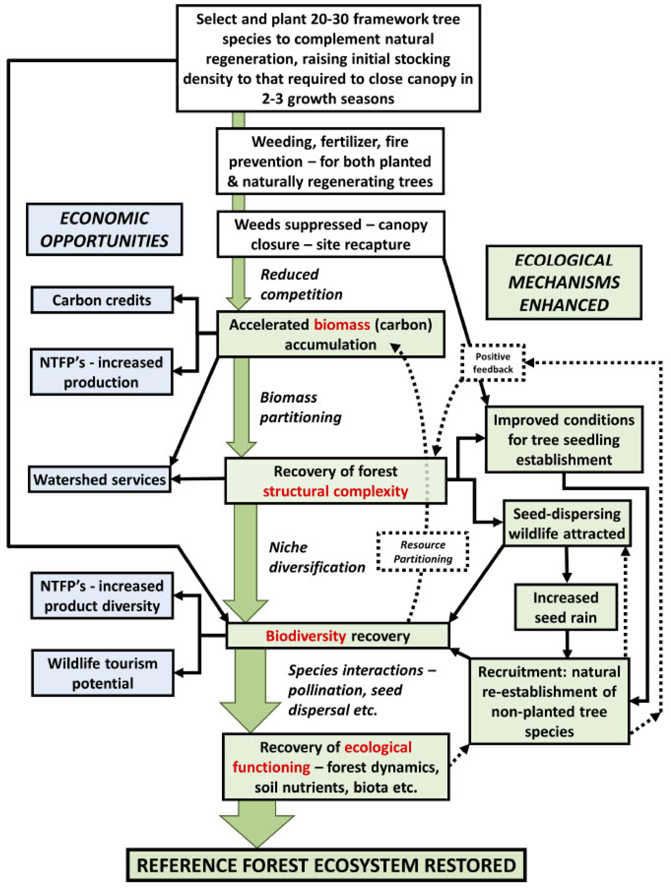
:1. Introduction
2. Materials and Methods
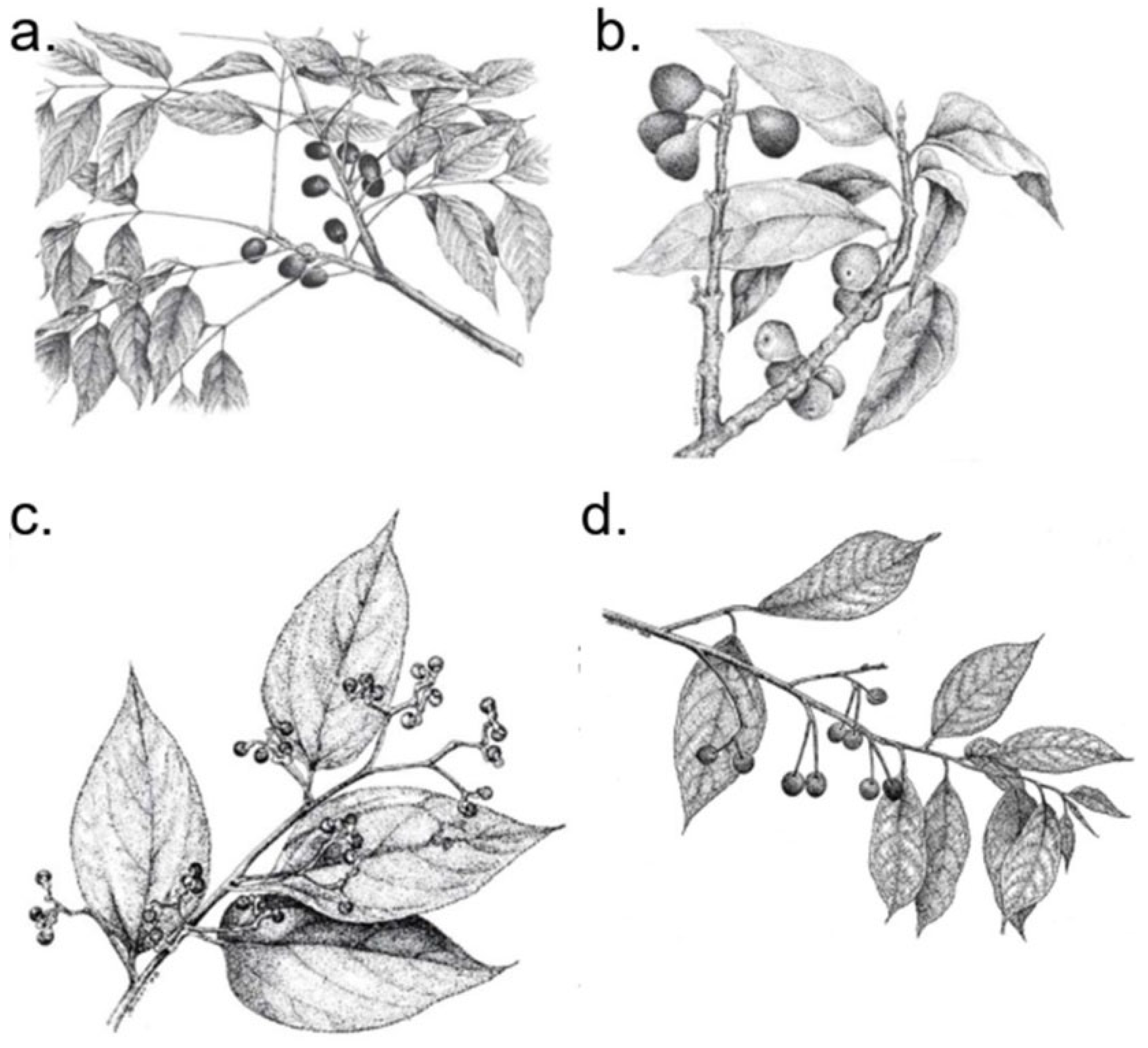
2.1. Studied Species
2.2. Data Collection
2.3. Species Location Record Preparation
2.4. Climatic Data Preparation
2.5. Modelling
3. Results
3.1. Model Performance and Potential Distributions of Four Studied Species
3.2. Importance of Climatic Variables
4. Discussion
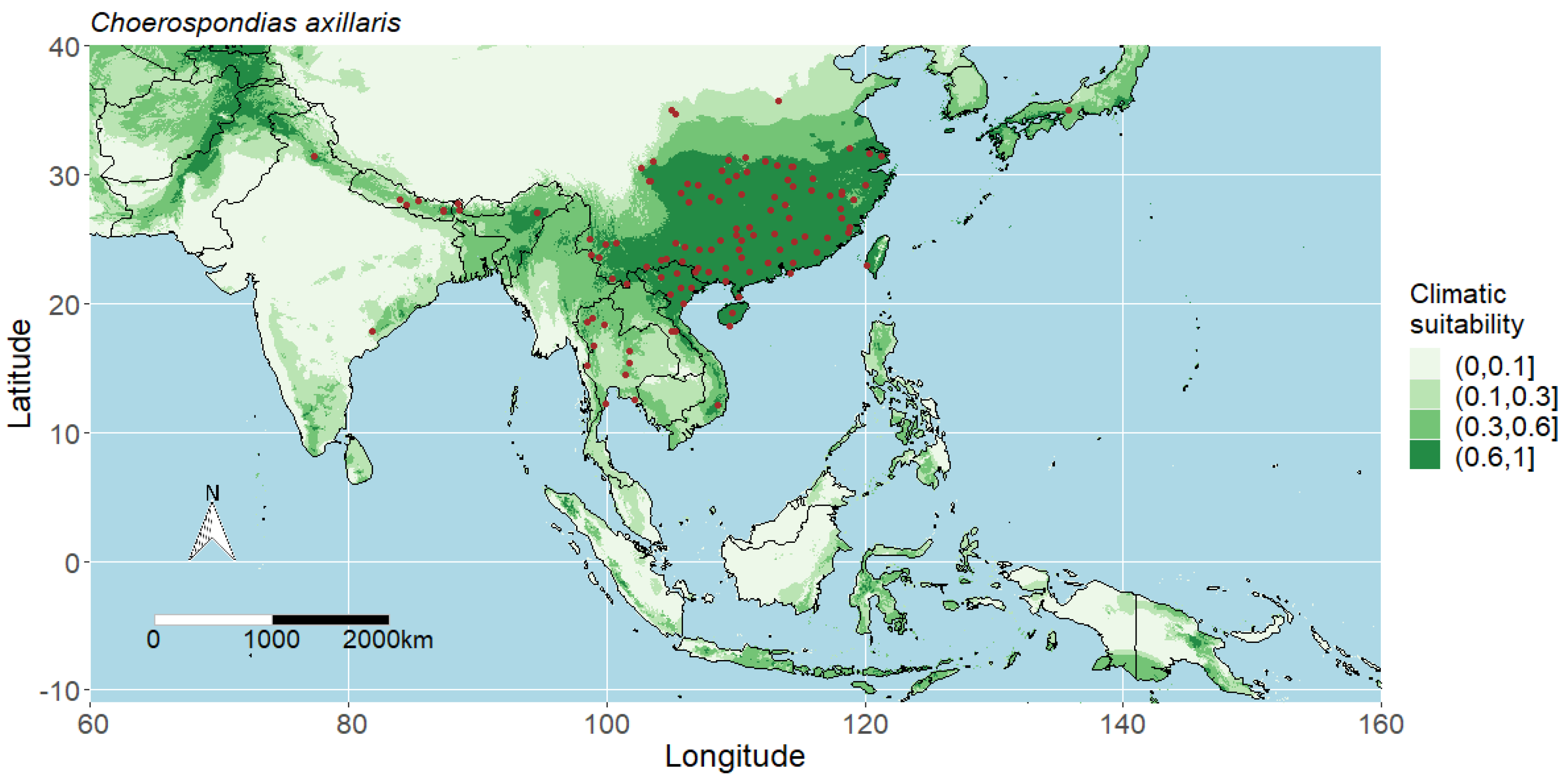
4.1. Interpreting the Maps
4.2. Predicted Potential Distribution of Choerospondias Axillaris and Contributing Variables
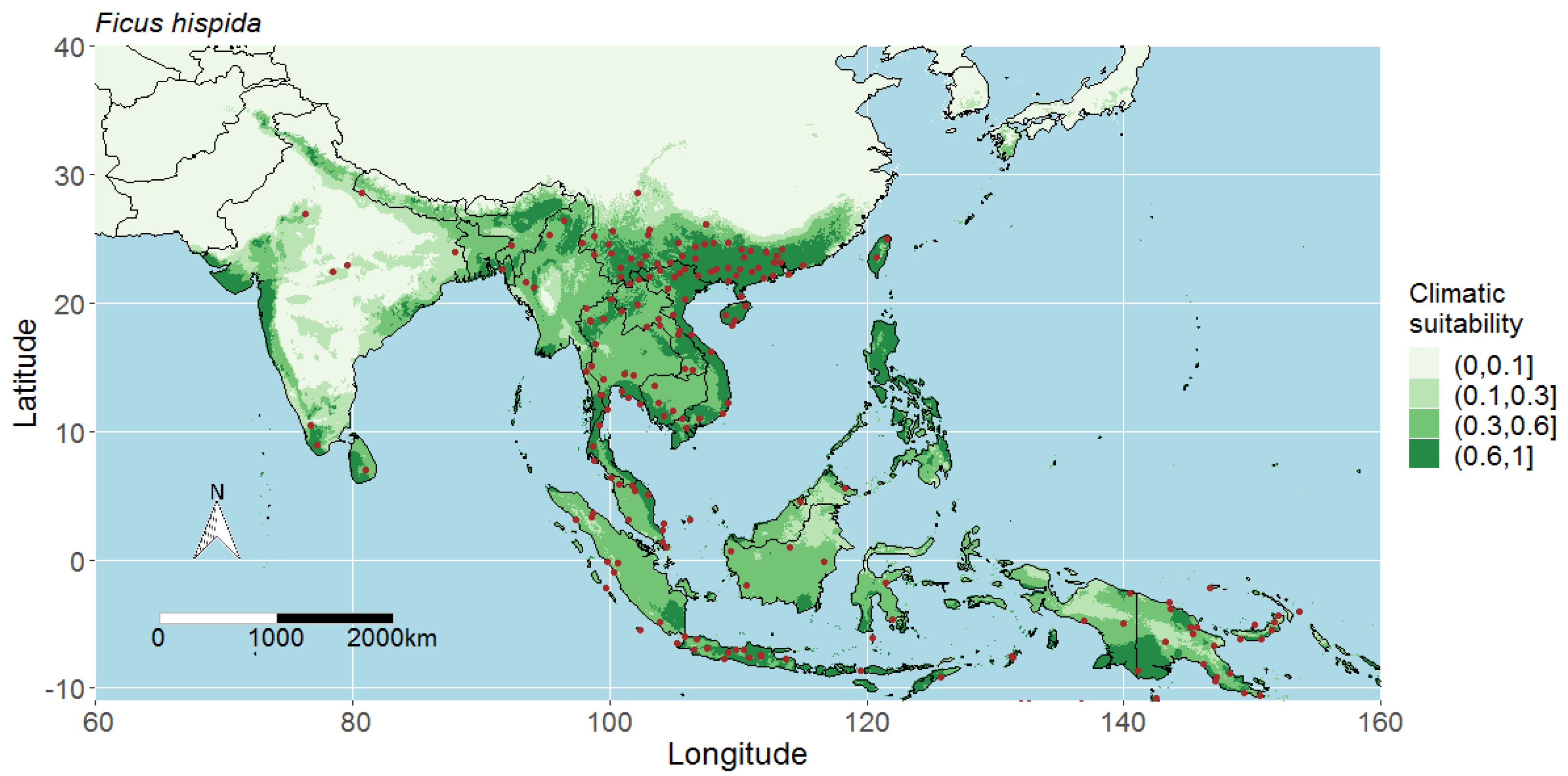
4.3. Predicted Potential Distribution of Ficus Hispida and Contributing Variables
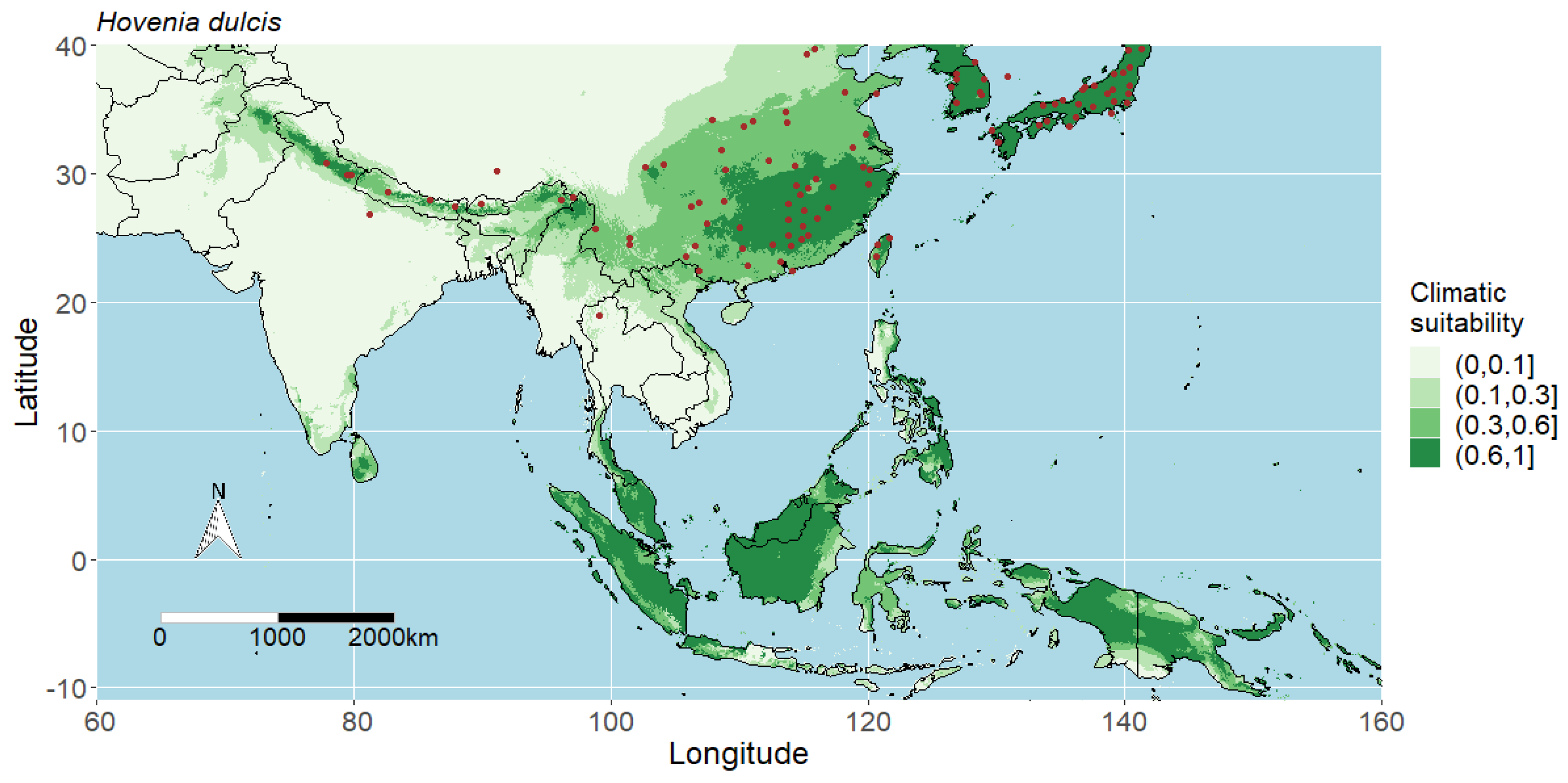
4.4. Predicted Potential Distribution of Hovenia Dulcis and Contributing Variables
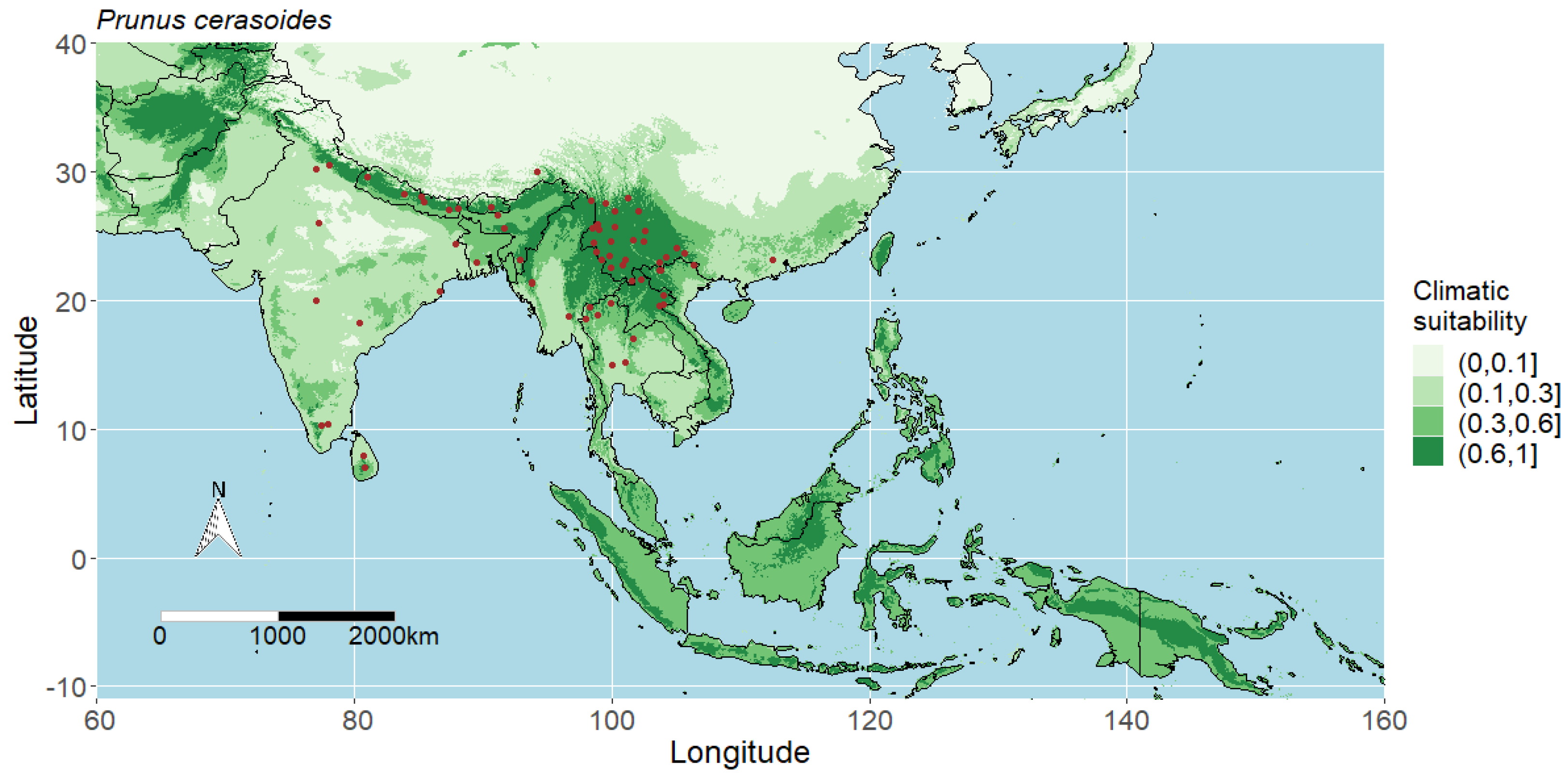
4.5. Predicted Potential Distribution of Prunus Cerasoides and Contributing Variables
4.6. Study Limitations and Future Direction for Species Distribution Modelling for Forest Restoration
5. Conclusions
Supplementary Materials
Author Contributions
Funding
Institutional Review Board Statement
Informed Consent Statement
Data Availability Statement
Acknowledgments
Conflicts of Interest
References
- Elliott, S.; Blakesley, D.; Hardwick, K. Restoring Tropical Forests: A Practical Guide; Royal Botanic Gardens, Kew: London, UK, 2013; p. 344. [Google Scholar]
- Catterall, C.P.; Kanowski, J.; Wardell-Johnson, G.W. Biodiversity and New Forests: Interacting Processes, Prospects and Pitfalls of Rainforest Restoration. In Living in a Dynamic Tropical Forest Landscape; Stork, N.E., Turton, S.M., Eds.; Wiley-Blackwell: New York, NY, USA, 2009; pp. 510–525. [Google Scholar]
- Tucker, N.I.J.; Simmons, T. Restoring a rainforest habitat linkage in north Queensland: Donaghy’s Corridor. Ecol. Manag. Restor. 2009, 10, 98–112. [Google Scholar] [CrossRef]
- Lewis, S.L.; Wheeler, C.E.; Mitchard, E.T.A.; Koch, A. Restoring natural forests is the best way to remove atmospheric carbon. Nature 2019, 568, 25–28. [Google Scholar] [CrossRef] [PubMed]
- IUCN. Restore Our Future: The Bonn Challenge. Available online: https://www.bonnchallenge.org/ (accessed on 18 May 2020).
- UNEP; FAO. The UN Decade on Ecosystem Restoration 2021–2030. Available online: https://wedocs.unep.org/bitstream/handle/20.500.11822/30919/UNDecade.pdf?sequence=11 (accessed on 6 July 2020).
- United Nations. Report of the Conference of the Parties on Its Thirteenth Session. In Proceedings of the Conference of the Parties on Its Thirteenth Session, Bali, Indonesia, 3–15 December 2007. [Google Scholar]
- United Nations. Report of the Conference of the Parties on Its Sixteenth Session. In Proceedings of the Conference of the Parties on Its Sixteenth Session, Cancun, Mexico, 29 November–10 December 2010. [Google Scholar]
- Lamb, D. Large-Scale Forest Restoration; Routledge: London, UK, 2014. [Google Scholar]
- Barlow, J.; Gardner, T.A.; Araujo, I.S.; Ávila-Pires, T.C.; Bonaldo, A.B.; Costa, J.E.; Esposito, M.C.; Ferreira, L.V.; Hawes, J.; Hernandez, M.I.M.; et al. Quantifying the biodiversity value of tropical primary, secondary, and plantation forests. Proc. Natl. Acad. Sci. USA 2007, 104, 18555–18560. [Google Scholar] [CrossRef] [PubMed] [Green Version]
- Goosem, S.; Tucker, N.I.J. Repairing the Rainforest, 2nd ed.; Wet Tropics Management Authority and Biotropica Australia Pty. Ltd: Cairns, Australia, 2013; p. 153. [Google Scholar]
- Sobon, K. Identifying Framework Tree Species for Restoring Forest Ecosystems in Siem Reap Province; Royal University of Agriculture: Phnom Penh, Cambodia, 2013. [Google Scholar]
- Harrison, R.; Swinfield, T. Restoration of logged humid tropical forests: An experimental programme at Harapan Rainforest, Indonesia. Trop. Conserv. Sci. 2015, 8, 4–16. [Google Scholar] [CrossRef] [Green Version]
- Weyerhaeuser, H.; Kahrl, F. Planting trees on farms in Southwest China: Enhancing rural economies and the environment. Mt. Res. Dev. 2006, 26, 205–208. [Google Scholar] [CrossRef] [Green Version]
- Marshall, A. (Udzungwa Forest Project, Morogoro, Tanzania). Restoration Project in Tanzania. Personal communication, 2021.
- WeForest. WeForest Project Philippines: Restoring the Sarangani Forest. Available online: https://www.weforest.org/project/philippines (accessed on 16 May 2020).
- Toktang, T. The Effects of Forest Restoration on the Species Diversity and Composition of a Bird Community in Doi Suthep-Pui National Park Thailand from 2002–2003; Chiang Mai University: Chaing Mai, Thailand, 2005. [Google Scholar]
- Sinhaseni, K. Natural Establishment of Tree Seedlings in Forest Restoration Trials at Ban Mae Sa Mai, Chiang Mai Province; Chiang Mai University: Chiang Mai, Thailand, 2008. [Google Scholar]
- Jantawong, K.; Elliott, S.; Wangpakapattanawong, P. Above-ground carbon sequestration during restoration of upland evergreen forest in northern Thailand. Open J. For. 2017, 7, 157–171. [Google Scholar] [CrossRef] [Green Version]
- Kavinchan, N.; Wangpakapattanawong, P.; Elliott, S.; Chairuangsri, S.; Pinthong, J. Use of the framework species method to restore carbon flow via litterfall and decomposition in an evergreen tropical forest ecosystem, northern Thailand. Kasetsart J.-Nat. Sci. 2015, 49, 639–650. [Google Scholar]
- Di Sacco, A.; Hardwick, K.A.; Blakesley, D.; Brancalion, P.H.S.; Breman, E.; Cecilio Rebola, L.; Chomba, S.; Dixon, K.; Elliott, S.; Ruyonga, G.; et al. Ten golden rules for reforestation to optimize carbon sequestration, biodiversity recovery and livelihood benefits. Glob. Chang. Biol. 2021, 27, 1328–1348. [Google Scholar] [CrossRef]
- Jantawong, K.; Kavinchan, N.; Wangpakapattanawong, P.; Elliott, S. Financial analysis of potential carbon value over 14 years of forest restoration by the framework species method. Forests 2022, 13, 144. [Google Scholar] [CrossRef]
- Gastón, A.; García-Viñas, J.I.; Bravo-Fernández, A.J.; López-Leiva, C.; Oliet, J.A.; Roig, S.; Serrada, R. Species distribution models applied to plant species selection in forest restoration: Are model predictions comparable to expert opinion? New For. 2014, 45, 641–653. [Google Scholar] [CrossRef]
- Thomas, E.; Alcázar Caicedo, C.; Moscoso, L.G.; Vásquez, A.; Osorio, L.F.; Salgado-Negret, B.; Ramírez, W. The importance of species selection and seed sourcing in forest restoration for enhancing adaptive capacity to climate change: Colombian tropical dry forest as a model. CBD Tech. Ser. 2017, 89, 122–132. [Google Scholar]
- Fremout, T.; Thomas, E.; Gaisberger, H.; Van Meerbeek, K.; Muenchow, J.; Briers, S.; Gutierrez-Miranda, C.E.; Marcelo-Peña, J.L.; Kindt, R.; Atkinson, R.; et al. Mapping tree species vulnerability to multiple threats as a guide to restoration and conservation of tropical dry forests. Glob. Chang. Biol. 2020, 26, 3552–3568. [Google Scholar] [CrossRef] [PubMed]
- Hardwick, K.A.; Fiedler, P.; Lee, L.C.; Pavlik, B.; Hobbs, R.J.; Aronson, J.; Bidartondo, M.; Black, E.; Coates, D.; Daws, M.I.; et al. The role of botanic gardens in the science and practice of ecological restoration. Conserv. Biol. 2011, 25, 265–275. [Google Scholar] [CrossRef] [PubMed]
- Sinclair, S.J.; White, M.D.; Newell, G.R. How useful are species distribution models for managing biodiversity under future climates? Ecol. Soc. 2010, 15, 8. [Google Scholar] [CrossRef]
- Elliott, S.; Navakitbumrung, P.; Kuarak, C.; Zangkum, S.; Anusarnsunthorn, V.; Blakesley, D. Selecting framework tree species for restoring seasonally dry tropical forests in northern Thailand based on field performance. For. Ecol. Manag. 2003, 184, 177–191. [Google Scholar] [CrossRef]
- Derived Dataset GBIF.org Filtered Export of GBIF Occurrence Data. Available online: https://doi.org/10.15468/dd.cg253q (accessed on 2 May 2022).
- Phillips, S.J.; Dudik, M.; Schapire, R.E. A Maximum Entropy Approach to Species Distribution Modeling. In Proceedings of the International Conference on Machine Learning (ICML’04), Banff, AB, Canada, 4–8 July 2004. [Google Scholar]
- Lissovsky, A.; Dudov, S. Species-distribution modeling: Advantages and limitations of its application. 2. MaxEnt. Biol. Bull. Rev. 2021, 11, 265–275. [Google Scholar] [CrossRef]
- Hao, T.; Elith, J.; Lahoz-Monfort, J.J.; Guillera-Arroita, G. Testing whether ensemble modelling is advantageous for maximising predictive performance of species distribution models. Ecography 2020, 43, 549–558. [Google Scholar] [CrossRef] [Green Version]
- Kaky, E.; Nolan, V.; Alatawi, A.; Gilbert, F. A comparison between Ensemble and MaxEnt species distribution modelling approaches for conservation: A case study with Egyptian medicinal plants. Ecol. Inform. 2020, 60, 101150. [Google Scholar] [CrossRef]
- Chiang Mai University Forest Restoration Research Unit. How to Plant a Forest: The Principels and Practice of Restoring Tropical Forests; Biology Department, Science Faculty, Chiang Mai University: Chiang Mai, Thailand, 2005. [Google Scholar]
- GeoNames Team. GeoNames. Available online: http://www.geonames.org/ (accessed on 21 July 2018).
- Hijmans, R.J.; Phillips, S.; Leathwick, J.; Elith, J. Dismo: Species Distribution Modeling. Available online: https://CRAN.R-project.org/package=dismo (accessed on 2 May 2022).
- R Core Team. R: A Language and Environment for Statistical Computing; R Foundation for Statistical Computing: Vienna, Austria, 2019. [Google Scholar]
- IPNI. International Plant Names Index. The Royal Botanic Gardens, Kew, Harvard University Herbaria and Libraries and Australian National Botanic Gardens; Available online: http://www.ipni.org (accessed on 2 May 2022).
- Hijmans, R.J.; Cameron, S.E.; Parra, J.L.; Jones, P.G.; Jarvis, A. Very high resolution interpolated climate surfaces for global land areas. Int. J. Climatol. 2005, 25, 1965–1978. [Google Scholar] [CrossRef]
- Fourcade, Y.; Engler, J.O.; Rödder, D.; Secondi, J. Mapping species distributions with MAXENT using a geographically biased sample of presence data: A performance assessment of methods for correcting sampling bias. PLoS ONE 2014, 9, e97122. [Google Scholar] [CrossRef] [Green Version]
- Leroy, B.; Meynard, C.N.; Bellard, C.; Courchamp, F. virtualspecies, an R package to generate virtual species distributions. Ecography 2015, 39, 599–607. [Google Scholar] [CrossRef]
- Phillips, S.J.; Dudík, M.; Schapire, R.E. Maxent Software for Modeling Species Niches and Distributions. Available online: https://biodiversityinformatics.amnh.org/open_source/maxent/ (accessed on 27 September 2019).
- Phillips, S.J. A Brief Tutorial on Maxent. Available online: https://biodiversityinformatics.amnh.org/open_source/maxent/ (accessed on 27 September 2019).
- Radosavljevic, A.; Anderson, R.P. Making better Maxent models of species distributions: Complexity, overfitting and evaluation. J. Biogeogr. 2014, 41, 629–643. [Google Scholar] [CrossRef]
- Phillips, S.J.; Anderson, R.P.; Schapire, R.E. Maximum entropy modeling of species geographic distributions. Ecol. Model. 2006, 190, 231–259. [Google Scholar] [CrossRef] [Green Version]
- Liu, Y.; Huang, P.; Lin, F.; Yang, W.; Gaisberger, H.; Christopher, K.; Zheng, Y. MaxEnt modelling for predicting the potential distribution of a near threatened rosewood species (Dalbergia cultrata Graham ex Benth). Ecol. Eng. 2019, 141, 105612. [Google Scholar] [CrossRef]
- Merow, C.; Smith, M.J.; Silander, J.A., Jr. A practical guide to MaxEnt for modeling species’ distributions: What it does, and why inputs and settings matter. Ecography 2013, 36, 1058–1069. [Google Scholar] [CrossRef]
- Guatum, K.H. Lapsi (Choerospondias axillaris) emerging as a commercial non-timber forest product in the hills of Nepal. In Forest Products, Livelihoods and Conservation: Case Studies of Non-Timber Forest Product Systems—Asia; Kusters, K., Belcher, B., Eds.; Center for International Forestry Research: Bogor Regency, Indonesia, 2004; Volume 1, pp. 114–129. [Google Scholar]
- Chanthorn, W.; Brockelman, W. Seed dispersal and seedling recruitment in the light-demanding tree Choerospondias axillaris in old-growth forest in Thailand. ScienceAsia 2008, 34, 129–135. [Google Scholar] [CrossRef] [Green Version]
- Invasive Species Specialist Group. Global Invasive Species Database; Invasive Species Specialist Group: Rome, Italy, 2020. [Google Scholar]
- Rojo, J.P.; Pitargue, F.C.; Sosef, M.S.M.; Ficus Hispida, L.F. Plant Resources of South-East Asia No 12: Medicinal and Poisonous Plants; de Padua, L.S., Bunyapraphatsara, N., Lemmens, R.H.M.J., Eds.; PROSEA Foundation: Bogor, Indonesia, 1999; Volume 12. [Google Scholar]
- Voris, H.K. Special paper 2: Maps of Pleistocene sea levels in Southeast Asia: Shorelines, river systems and time durations. J. Biogeogr. 2000, 27, 1153–1167. [Google Scholar] [CrossRef] [Green Version]
- Yang, D.; Peng, Y.; Song, Q.; Zhang, G.; Wang, R.; Zhao, T.; Wang, Q. Pollination biology of Ficus hispida in the tropical rainforests of Xishuangbanna, China. Acta Bot. Sin. 2002, 44, 519–526. [Google Scholar]
- Maxwell, J.F. Botanical Notes on the Flora of Thailaod: 4. Nat. Hist. Bull. Siam Soc. 1994, 42, 4. [Google Scholar]
- Kopachon, S.; Suriya, K.; Hardwick, K.; Pakaad, G.; Maxwell, J.F.; Anusarnsunthorn, V.; Blakesley, D.; Garwood, N.C.; Elliott, S. Forest restoration research in northern Thailand, 1. The fruits, seeds and seedlings of Hovenia dulcis Thunb. (Rhamnaceae). Nat. Hist. Bull. Siam Soc. 1996, 44, 12. [Google Scholar]
- Hitchcock, D.; Elliott, S. Forest restoration research in northern Thailand, III : Observations of birds feeding in mature Hovenia dulcis Thunb. (Rhamnaceae). Nat. Hist. Bull. Siam Soc. 1999, 47, 149–152. [Google Scholar]
- Zenni, R.D.; Ziller, S.R. An overview of invasive plants in Brazil. Braz. J. Bot. 2011, 34, 431–446. [Google Scholar] [CrossRef] [Green Version]
- Hendges, C.; Fortes, V.B.; Dechoum, M. Consumption of the invasive alien species Hovenia dulcis Thumb. (Rhamnaceae) by Sapajus nigritus Kerr, 1792 in a protected area in southern Brazil. Rev. Bras. De Zoociências 2012, 14, 255–260. [Google Scholar]
- Penny, J. Plant 100: Hovenia Dulcis Thunb. (Rhamnaceae); Department of Plant Sciences, University of Oxford: Oxford, UK, 2020. [Google Scholar]
- Bergamin, R.S.; Gama, M.; Almerão, M.; Hofmann, G.S.; Anastácio, P.M. Predicting current and future distribution of Hovenia dulcis Thunb. (Rhamnaceae) worldwide. Biol. Invasions 2022. [Google Scholar] [CrossRef]
- The Forest Restoration Research Unit. Tree Seeds and Seedlings for Restoring Forests in Northern Thailand; Kerby, J., Elliott, S., Blakesley, D., Anusarnsunthorn, V., Eds.; Biology Department, Science Faculty, Chiang Mai University: Chiang Mai, Thailand, 2000; p. 152. [Google Scholar]
- Mapaura, A.; Timberlake, J. (Eds.) A Checklist of Zimbabwean Vascular Plants; Southern African Botanical Diversity Network Report No. 33 Sabonet; Southern African Botanical Diversity Network (SABONET): Pretoria, South Africa; Available online: http://opus.sanbi.org/bitstream/20.500.12143/5966/1/Mapaura_et_al_2004.pdf (accessed on 2 May 2022).
- Atlas of Living Australia. Species Page. 2020. Available online: https://bie.ala.org.au/species/NZOR-6-116741 (accessed on 14 August 2020).
- Herbarium, A. Prunus cerasoides Records. 2020. Available online: https://scd.landcareresearch.co.nz/ (accessed on 17 May 2020).
- Kobayashi, Y. Cherry blossoms in Japan. Jpn. Agric. Res. Q. 1983, 17, 5. [Google Scholar]
- Daru, B.H.; Park, D.S.; Primack, R.B.; Willis, C.G.; Barrington, D.S.; Whitfeld, T.J.S.; Seidler, T.G.; Sweeney, P.W.; Foster, D.R.; Ellison, A.M.; et al. Widespread sampling biases in herbaria revealed from large-scale digitization. New Phytol. 2018, 217, 939–955. [Google Scholar] [CrossRef] [PubMed] [Green Version]
- Phillips, S.J. Transferability, sample selection bias and background data in presence-only modelling: A response to Peterson et al. (2007). Ecography 2008, 31, 272–278. [Google Scholar] [CrossRef]
- Velazco, S.J.E.; Galvão, F.; Villalobos, F.; De Marco Júnior, P. Using worldwide edaphic data to model plant species niches: An assessment at a continental extent. PLoS ONE 2017, 12, e0186025. [Google Scholar] [CrossRef] [PubMed] [Green Version]
- Zuquim, G.; Costa, F.R.C.; Tuomisto, H.; Moulatlet, G.M.; Figueiredo, F.O.G. The importance of soils in predicting the future of plant habitat suitability in a tropical forest. Plant Soil 2020, 450, 151–170. [Google Scholar] [CrossRef] [Green Version]
- Dubuis, A.; Giovanettina, S.; Pellissier, L.; Pottier, J.; Vittoz, P.; Guisan, A. Improving the prediction of plant species distribution and community composition by adding edaphic to topo-climatic variables. J. Veg. Sci. 2013, 24, 593–606. [Google Scholar] [CrossRef]
- Thuiller, W. On the importance of edaphic variables to predict plant species distributions–limits and prospects. J. Veg. Sci. 2013, 24, 591–592. [Google Scholar] [CrossRef] [PubMed] [Green Version]
- Trisurat, Y.; Shrestha, R.P.; Kjelgren, R. Plant species vulnerability to climate change in Peninsular Thailand. Appl. Geogr. 2011, 31, 1106–1114. [Google Scholar] [CrossRef] [Green Version]
- Khan, A.M.; Li, Q.; Saqib, Z.; Khan, N.; Habib, T.; Khalid, N.; Majeed, M.; Tariq, A. MaxEnt modelling and impact of climate change on habitat suitability variations of economically important Chilgoza Pine (Pinus gerardiana Wall.) in South Asia. Forests 2022, 13, 715. [Google Scholar] [CrossRef]


| Species | Family | Elevation (m asl) 1 | Framework Species Assessment 2 | |||||
|---|---|---|---|---|---|---|---|---|
| Lower | Upper | Survival 3 | Growth 4 | Weed Suppression 5 | Fire Resilience 6 | Attraction to Seed Dispersers 7 | ||
| Choerospondias axillaris (Roxb.) B.L. Burtt and A.W. Hill | Anacardiaceae | 460 | 1600 | E | E | A | E | Flowering and fruiting from 4th year. Fruits attract seed-dispersing mammals. |
| Ficus hispida L.f. | Moraceae | 60 | 1525 | E | A | E | E | Figs from 3rd year attract seed-dispersing birds/squirrels. |
| Hovenia dulcis Thunb. | Rhamnaceae | 1025 | 1300 | E | E | E | E | Fruit and infructescence attract seed-dispersing birds but flowers late: >8 years after planting. |
| Prunus cerasoides Buch.-Ham. ex D. Don | Rosaceae | 1050 | 1750 | E | E | E | A | Flowers, fruit, and bird nests within 3 years. Fruits attract seed-dispersing birds. |
| Species | Herbarium Records | GBIF Records with Coordinate Data 1 | Records within the Native Range | Subsampled Records | Native Geographical Extent of Location Data | Range Description |
|---|---|---|---|---|---|---|
| C. axillaris | 57 | 361 | 183 | 116 | Longitude 77–142° E Latitude 18–40° N | India to China Southeast/south-central China to Thailand |
| F. hispida | 60 | 1221 | 756 | 236 | Longitude 76–154° E Latitude 20°S–38° N | India to Australia Australia to Southeast/south-central China |
| H. dulcis | 70 | 637 | 391 | 101 | Longitude 77–136° E Latitude 11–36° N | India to Japan Japan and China to Thailand |
| P. cerasoides | 46 | 213 | 139 | 68 | Longitude 76–113° E Latitude 6–31° N | India to Thailand South China to Thailand |
| Total | 234 | 2432 | 1481 | 524 |
| Abbreviation | Variables (Unit) | Note | Used in Modelling |
|---|---|---|---|
| Bio1 | Annual mean temperature (°C) | ||
| Bio2 | Mean diurnal range (mean of monthly) (°C) | max temp–min temp | ✓ |
| Bio3 | Isothermality (%) 1 | (Bio2/Bio7) × 100 | ✓ |
| Bio4 | Temperature seasonality (°C) 2 | standard deviation | |
| Bio5 | Max temperature of warmest month (°C) | ||
| Bio6 | Min temperature of coldest month (°C) | ||
| Bio7 | Temperature annual range (°C) | Bio5–Bio6 | |
| Bio8 | Mean temperature of wettest quarter (°C) | ✓ | |
| Bio9 | Mean temperature of driest quarter (°C) | ✓ | |
| Bio10 | Mean temperature of warmest quarter (°C) | ✓ | |
| Bio11 | Mean temperature of coldest quarter (°C) | ||
| Bio12 | Annual precipitation (mm) | ||
| Bio13 | Precipitation of wettest month (mm) | ✓ | |
| Bio14 | Precipitation of driest month (mm) | ✓ | |
| Bio15 | Precipitation seasonality (%) 3 | coefficient of variation | ✓ |
| Bio16 | Precipitation of wettest quarter (mm) | ||
| Bio17 | Precipitation of driest quarter (mm) | ||
| Bio18 | Precipitation of warmest quarter (mm) | ✓ | |
| Bio19 | Precipitation of coldest quarter (mm) | ✓ |
| Species | Average AUC | Permutation Importance (Normalized Percentage) and Suitable Range of Variables | |||||
|---|---|---|---|---|---|---|---|
| (1 Standard Deviation) | The First | Suitable Range (Optimal Value) | The Second | Suitable Range (Optimal Value) | The Third | Suitable Range (Optimal Value) | |
| C. axillaris | 0.783 (0.062) | Mean temperature of driest quarter (36.3%) | 4.7–18.8 °C (13.9 °C) | Precipitation of driest month (19.3%) | 8.8–81.6 mm (22.5 mm) | Precipitation of wettest month (11.8%) | 161.0–397.7 mm (215.3 mm) |
| F. hispida | 0.811 (0.039) | Precipitation of driest month (20%) | ≥7.9 mm (14.3 mm) | Precipitation seasonality (17.4%) | 21–95% (72.4%) | Mean temperature of driest quarter (°C) (15.4%) | 11.3–27.0 °C (25.6 °C) |
| H. dulcis | 0.830 (0.059) | Precipitation of coldest quarter (32.3%) | ≥87 mm (558 mm) | Precipitation of warmest quarter (24.2%) | 448.0–2127.2 mm (526.0 mm) | Mean temperature of wettest quarter (9.6%) | 18.5–25.1 °C (23.1 °C) |
| P. cerasoides | 0.782 (0.079) | Mean temperature of driest quarter (59.5%) | 4.3–18.8 °C (11.1 °C) | Mean temperature of warmest quarter (27.9%) | 12.7–25.6 °C (18.4 °C) | Isothermality (9.6%) | 43.3–62.6% (49.2%) |
Publisher’s Note: MDPI stays neutral with regard to jurisdictional claims in published maps and institutional affiliations. |
© 2022 by the authors. Licensee MDPI, Basel, Switzerland. This article is an open access article distributed under the terms and conditions of the Creative Commons Attribution (CC BY) license (https://creativecommons.org/licenses/by/4.0/).
Share and Cite
Tiansawat, P.; Elliott, S.D.; Wangpakapattanawong, P. Climate Niche Modelling for Mapping Potential Distributions of Four Framework Tree Species: Implications for Planning Forest Restoration in Tropical and Subtropical Asia. Forests 2022, 13, 993. https://doi.org/10.3390/f13070993
Tiansawat P, Elliott SD, Wangpakapattanawong P. Climate Niche Modelling for Mapping Potential Distributions of Four Framework Tree Species: Implications for Planning Forest Restoration in Tropical and Subtropical Asia. Forests. 2022; 13(7):993. https://doi.org/10.3390/f13070993
Chicago/Turabian StyleTiansawat, Pimonrat, Stephen D. Elliott, and Prasit Wangpakapattanawong. 2022. "Climate Niche Modelling for Mapping Potential Distributions of Four Framework Tree Species: Implications for Planning Forest Restoration in Tropical and Subtropical Asia" Forests 13, no. 7: 993. https://doi.org/10.3390/f13070993
APA StyleTiansawat, P., Elliott, S. D., & Wangpakapattanawong, P. (2022). Climate Niche Modelling for Mapping Potential Distributions of Four Framework Tree Species: Implications for Planning Forest Restoration in Tropical and Subtropical Asia. Forests, 13(7), 993. https://doi.org/10.3390/f13070993