Abstract
In polarimetric interferometric SAR (PolInSAR) technology, the random volume over ground (RVoG) model establishes the mapping relationship between polarimetric complex coherence and forest biophysical parameters (e.g., forest height). However, due to speckle noise and the finite multilooking effect, the real observed coherence region in the complex unitary circle (CUC) is an ellipse, which is biased by the ideal noise-free coherence region represented as a straight line by the RVoG model. Multilooking processing can reduce speckle noise at the cost of resolution loss. Therefore, this paper analyzes the influence of different multilooking sizes on forest height inversion. Experimental results show that the accuracy of forest height inversion first increases and then decreases with the increase in multilooking size, which means there exists an optimal size for PolInSAR forest estimation. From statistical analysis of the forest height estimation error, inversion accuracy mainly depends on estimation bias rather than estimation variance. This is mainly because, in a homogeneous forest area, a large multilooking size helps to reduce the statistical bias effect; in the textured area, the inversion accuracy benefits from a small multilooking size for avoiding the mixing of multiple types of ground targets.
1. Introduction
Forests play a vital role in the global carbon and oxygen cycle and contain many complex parameters; among them, forest height is a top priority for forest monitoring [1]. Polarimetric interferometric synthetic aperture radar (PolInSAR) technology is one of the most important methods for forest height inversion and obtains both polarimetric characteristics and interferometric information [2,3] over forest areas. For forest areas, the polarimetric characteristics are sensitive to the dielectric properties, shape distribution, and directionality of the volume scatterers, while the interferometric information is sensitive to the vertical distribution and height changes of vegetation scatterers. Therefore, PolInSAR technology has become the most commonly used remote sensing method for estimating forest height [4,5].
Widely used technology based on SAR data for forest height inversion includes random volume over ground (RVoG)-based inversion [6,7], polarization coherence tomography (PCT) [8,9], SAR tomography (TomoSAR) [10,11], and so on. Among them, the RVoG model is represented as the most extensive polarimetric coherent scattering model in PolInSAR technology. Considering different factors, many improved algorithms based on the RVoG model have been developed consecutively, such as temporal decorrelation (RVoG+TD) [12,13], volume temporal decorrelation (RVoG+VTD) [14,15], random motion over ground (RMoG) [16,17], slope (S-RVoG) [18], and varying extinction (VERVoG) [19]. Essentially, the RVoG model abstracts the forest area into both a forest layer and a surface layer and establishes the functional relationship between the polarimetric complex coherence observations and forest biophysical parameters.
In order to estimate forest height, many algorithms based on the RVoG model have been proposed. Papathanassiou et al. considered three polarimetric complex coherences with Maximum Coherence Difference (MCD) as the input observations and performed a nonlinear optimization to estimate forest height [20]. However, to avoid the rank deficiency problem in the above six-dimensional nonlinear optimization processing, Cloude et al. proposed the three-stage algorithm [21]. This algorithm considers the geometric expression of RVoG in the complex unitary circle (CUC) and uses least square line fitting to estimate the ground phase. To further reduce the number of unknown parameters, the ground-to-volume scattering ratio can be supposed to be 0, and a two-dimensional lookup table is used to calculate forest height and the extinction coefficient. Dubois-Fernandez et al. [22] and Garestier et al. [23] proposed an improved three-stage algorithm based on long-wavelength SAR, fixed to the extinction coefficient instead of the ground-to-volume scattering ratio because the scene contained considerable ground scattering contribution. Compared to six-dimensional nonlinear iterations, both three-stage algorithms take into account the geometric properties of the RVoG model, and the reliability and practicality have been improved. In addition, Zhu et al. extended the least squares adjustment from the real domain to the complex domain and proposed the complex least squares algorithm and obtained more accurate forest height results [24].
In PolInSAR technology, the coherence set corresponds to the coherence values of all polarimetric channels, which shows a continuous region in the CUC, defined as the coherence region. Usually, the coherence region is applied to analyze the geometrical distribution of all possible coherence values in the CUC. The coherence region expressed by the RVoG model is a line segment in the complex plane, defined as the coherent line segment in this paper. However, polarimetric complex coherence is easily affected by inherent speckle noise in the coherent imaging system [25,26], and hence the coherent line segment degenerates into an ellipse distributed on both sides of the coherent line segment, defined as the coherent ellipse in this paper. In practice, due to the finite multilooking effect or practical scene heterogeneity, this coherent ellipse is further biased by the coherent line segment in the complex plane, and it then results in a loss of image resolution and detailed information. Therefore, it is necessary to analyze the influence of different multilooking sizes on forest height inversion accuracy. Based on the P-band PolInSAR data provided by the AfriSAR2016 campaign, this paper evaluates and analyzes multiple Boxcar filtering sizes ranging from 5 × 5 to 25 × 25, and employs the fixed extinction coefficient algorithm to estimate forest height. Additionally, forest height results after Boxcar filtering are compared to those after refined Lee filtering [27] and intensity driven adaptive neighborhood (IDAN) [28] filtering.
The rest of this paper is organized as follows. Section 2 explains the RVoG model and fixed extinction coefficient-based forest height inversion. In Section 3, there is an overview of the study area and data sets. Results and analysis are presented in Section 4. Finally, the major conclusions of this work are given in Section 5.
2. Methodology
2.1. PolInSAR Matrix Generation
The scattering matrix can usually be used for describing the full polarimetric information of a single target. In the case of linear horizontal and vertical polarization bases, the Sinclair scattering matrix is expressed as follows [29]:
For a reciprocal target matrix, in the monostatic backscattering case, the reciprocity constrains the matrix to being symmetrical, that is, . The corresponding complex Pauli basis vector is [29]:
where denotes the transpose. The complex Pauli basis scattering vectors of two images construct the six-element complex scattering target vector . Therefore, the PolInSAR data is formulated into a 6 × 6 interferometric coherency matrix by and its conjugate transpose [29]:
where denotes the spatial multilook average and is the complex conjugate. and are master and slave polarimetric coherency matrixes that contain full polarimetric information, respectively. denotes the interferometric cross correlation matrix. In order to acquire the interferogram of a polarization channel between two observations, a normalized complex projection vector is introduced. For full-polarimetric SAR images, is parameterized as follows [29]:
where , , , and are the polarimetric covariance matrix written in terms of the so-called polarimetric intercorrelation parameters [30]. The complex Pauli basis scattering vectors and can be projected onto the given complex projection vectors and , and the corresponding polarimetric image and can be obtained, i.e., and . Thus, for both polarimetric channels and , the complex polarimetric interferometric coherence can be formed [29]:
2.2. RVoG Model
To describe the scattering scene of the two-layer structure in a forest area, the RVoG model establishes the mapping function between the polarimetric complex coherence and the forest biophysical parameters (as shown in Figure 1) [21]:
where denotes the volume coherence in a polarimetric channel , which includes contributions from both the volume and ground layers, is the underlying ground phase, denotes the ground-to-volume amplitude ratio, and represents the volume-only coherence. Considering the impact of terrain slope on forest height estimation, can be expressed in terms of [18]:
where represents the extinction coefficient, denotes forest height, is the local range terrain slope, and is the local incidence angle calculated by the nominal incidence angle (i.e., ). is the local effective vertical wavenumber given as follows [21]:
where represents the radar wavelength, denotes the perpendicular baseline, and is slant range distance.
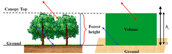
Figure 1.
The RVoG model. Note that the red and blue arrows represent the volume and ground scattering procedure, respectively.
From (6), when the radar response is dominated by ground contribution, the scattering phase center is located closer to the ground, i.e., , and complex coherence is equal to the underlying ground phase: . At the other extreme, when the radar response is dominated by volume scattering, without the presence of the ground (), the complex coherence is equal to the volume-only coherence with the underlying ground phase: . Therefore, from the perspective of the geometric interpretation, the RVoG model can be expressed as a linear function of both real and imaginary parts of the polarimetric complex coherence set and corresponds to a line segment in the CUC.
2.3. Fixed Extinction Coefficient-Based Forest Height Inversion
Due to the large amount of penetration into the vegetation volume at the P-band, the fixed extinction coefficient algorithm is an inversion better suited to the forest scene and data exploited in this study [22,23]. The inversion process of the fixed extinction coefficient algorithm is:
- (1)
- Line fitting. Common polarimetric complex coherences (i.e., , , , , ) and complex coherences and based on the phase diversity (PD) algorithm [31] are selected, and the total least square line fitting is then used for obtaining the coherent line segment;
- (2)
- Ground phase estimation. There are two intersections between the line segment and CUC, one of which is the ground phase. Thus, to determine the ground phase, Kugler et al. proposed a method-based [32]:where and are the two intersections between the line segment and CUC, respectively;
- (3)
- Forest height estimation. In order to avoid the influence of ground scattering contribution, the is used as the observation, and then a fixed extinction coefficient is used. Finally, the two-dimensional lookup table of forest height and ground-to-volume scattering ratio is established to estimate forest height [23]:
Compared to the traditional three-stage algorithm, the fixed extinction coefficient-based improved algorithm considers that the long-wavelength SAR scene contains considerable ground scattering contribution. This method is more suitable for the selected P-band SAR data in this paper, and effectively guarantees the accuracy of forest height inversion.
3. Study Areas and Data Sets
This paper selects two study areas, which are located in Mabounie (00°43′ S, 10°31′ E) and Mondah (00°35′ N, 9°18′ E) in Gabon, Africa. Mabounie covers an area of about 4.45 × 10⁴ km2 and is dominated by hilly landforms with relatively gentle fluctuations and the average forest height is about 30 m. Mondah covers an area of about 6.62 × 10⁴ km2 and is a relatively young forest with high variability in density and forest height is roughly between 5 m and 55 m.
The P-band full polarimetric SAR data over the two study areas were acquired from the framework of the European Space Agency (ESA) AfriSAR 2016 campaign. The German Aerospace Center’s F-SAR airborne system was used in this campaign. Two fully polarimetric SAR images were selected for the interferometric process from the Mabounie area. Similarly, two SAR images were also selected from the Mondah area. Table 1 shows the detailed system parameters of the selected SAR images. In addition, the airborne light detection and ranging (LiDAR) data covering the test areas were acquired from the National Aeronautics and Space Administration (NASA)’s Land, Vegetation, and Ice Sensor (LVIS) system, which was used to verify the accuracy of the inversion results, whose LiDAR footprint on the ground is around 20 m wide [32]. The mean of master and slave Pauli basis composite RGB (PauliRGB) images and LiDAR Canopy Height Model (CHM) products in the Mabounie and Mondah areas are shown in Figure 2 and Figure 3, respectively. Figure 3c shows the optical image of the Mondah area in 2016 acquired from Google Earth.

Table 1.
System parameters for Mabounie and Mondah from the AfriSAR 2016 campaign.
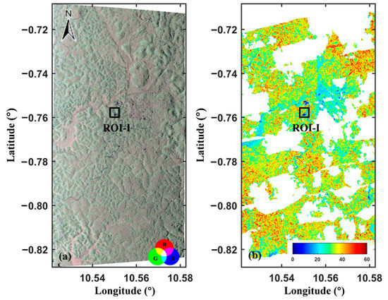
Figure 2.
Mabounie study area: (a) average of master and slave PauliRGB images; (b) LiDAR CHM. Note that in the quad-polarization, the red color is , blue color is the , and the green color is .
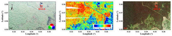
Figure 3.
Mondah study area: (a) average of master and slave PauliRGB images; (b) LiDAR CHM; (c) optical image.
In order to analyze the influence of different multilooking sizes on forest height inversion accuracy, the multiple Boxcar filtering sizes were designed to vary from 5 × 5 to 25 × 25, and the fixed extinction coefficient algorithm was applied to estimate forest height. The P-band data has strong penetration and a high ground scattering contribution, which is the result of a low extinction level [33]. Thus, the following experiment has fixed the extinction coefficient to be 0.1 dB/m. Finally, taking LiDAR CHM products as the reference data, we quantitatively analyze estimation accuracy of the forest height calculations.
4. Results and Analysis
We analyzed the influence of multilooking sizes or different filtering methods on forest height estimation in detail from the following four aspects: (1) numerical analysis based on backscattering intensity; (2) geometric interpretation based on coherence region; (3) error analysis based on statistical indicators; and (4) accuracy analysis of different filtering methods.
4.1. Numerical Analysis Based on Backscattering Intensity
For the detailed investigation, we selected a 200 × 200 pixels region of interest (ROI) labeled ROI-I (the black square box in Figure 2) and ROI-II (the red square box in Figure 3) from the Mabounie and Mondah areas. Figure 4a–c shows the pixel-wise forest height estimation error of ROI-I using different multilooking sizes (5 × 5, 9 × 9, 25 × 25), and the corresponding LiDAR results, PauliRGB image, and optical image is shown in Figure 4d–f. In ROI-II, the estimation errors of the 5 × 5 size, 11 × 11 size, 25 × 25 size, the corresponding LiDAR results, the PauliRGB image, and the optical image from Google Earth are shown in Figure 5.
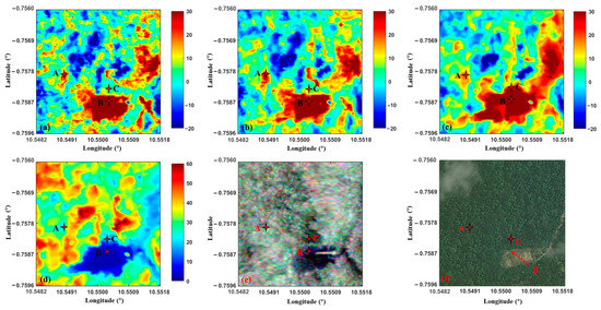
Figure 4.
Estimation error of forest height results under three sizes and LiDAR forest height results in Mabounie: (a) 5 × 5 size; (b) 9 × 9 size; (c) 25 × 25 size; (d) LiDAR forest height; (e) PauliRGB image; (f) optical image.
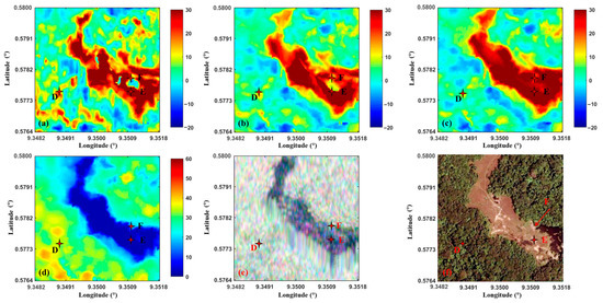
Figure 5.
Estimation error of forest height results under three sizes and LiDAR forest height results in Mondah: (a) 5 × 5 size; (b) 11 × 11 size; (c) 25 × 25 size; (d) LiDAR forest height; (e) PauliRGB images; (f) optical image.
To prove the influence of different multilooking sizes on single-baseline PolInSAR forest height inversion, this paper first analyzes the variation of backscattering intensity from different multilooking sizes. The section selects two pixels, specifically A (see Figure 4) and D (see Figure 5) from the homogeneous areas of ROI-I and ROI-II, respectively. We then use the HH channel to calculate the backscattering intensity of pixels A and D and the standard deviation of backscattering intensity centered on pixels A and D at each space, respectively, as shown in Figure 6. Note that this standard deviation is used to evaluate the spatial smoothness of intensity after filtering of different sizes. It can be seen from Figure 6 that as size increases, the backscattering intensities tend to be stable for each space, and spatial variation is also smaller and smaller.
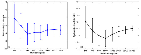
Figure 6.
Backscattering intensity and spatial variations of pixels at the HH channel for different multilooking sizes: (a) pixel A in Mabounie; (b) pixel D in Mondah.
Moreover, pixels B and C (see Figure 4) and pixels E and F (see Figure 5) belonging to the textured region are selected in ROI-I and ROI-II, respectively. We then calculated the backscattering intensity values under different multilooking sizes as shown in Figure 7. With the increase in multilooking size, backscattering intensity values for pixels B and C gradually became closer, and pixels E and F had a similar phenomenon. This explains how two pixels could be confused with each other and hence have similar values.
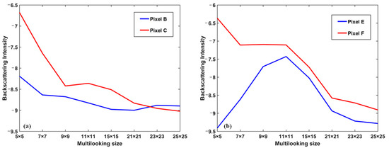
Figure 7.
Backscattering intensity of pixels at the HH channel for different multilooking sizes: (a) pixels B and C in Mabounie; (b) pixels E and F in Mondah.
4.2. Geometric Interpretation Based on Coherence Region
Generally, the estimation error of PolInSAR forest height mainly depends on estimation bias, which may be derived from the finite multilooking effect and multilooking average without any discrimination. In order to analyze the source of the estimation bias, we make a detailed analysis of the geometrical characteristics of the coherence region under different multilooking sizes from ROI-I and ROI-II.
To analyze the influence of the finite multilooking effect on bias for forest height inversion in detail we selected the same two pixels A (see Figure 4) and D (see Figure 5) from the homogeneous areas of ROI-I and ROI-II, respectively. The LiDAR forest heights of pixels A and D are 30.47 m and 33.14 m, respectively. It can be seen from Figure 4a–c and Figure 5a–c that the forest heights of pixels A and D are overestimated, but as the size increases, the phenomenon of overestimation weakens significantly. For pixel A, the estimation errors are 22.87 m, 15.74 m, and 9.57 m for the three sizes, respectively. Meanwhile, the estimation errors for the three sizes for pixel D are 20.85 m, 13.96 m, and 3.06 m, respectively. In the homogeneous area, bias reduction benefits from the large multilooking size. We then used a boundary sampling method to draw the contour of the coherence regions [34] for pixels A and D, obtained the farthest point pairs as the endpoints of the coherent line segment, and calculated the coherence amplitude at the HH channel, as shown in Figure 8. It can be seen from Figure 8 that, due to the existence of speckle noise, all polarimetric complex coherence sets are represented as a coherent elliptical region in the CUC. As the multilooking size increases, the coherence set shrinks and becomes flatter. The finite multilooking effect makes the observed coherence region biased due to the coherent line segment of the RVoG model. In a word, the aforementioned results have proved that a large multilooking size helps to reduce the statistical bias effect in a homogeneous forest area.
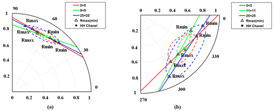
Figure 8.
Geometrical interpretation including the contour of the coherence regions, the endpoints of the coherent line segment, and the corresponding lines of pixels A and D under different multilooking sizes: (a) pixel A for 5 × 5, 9 × 9, and 25 × 25 sizes in the Mabounie area; (b) pixel D for 5 × 5, 11 × 11, and 25 × 25 sizes in the Mondah area. Note that Rmax is the endpoint near the ground phase, Rmin is the endpoint away from the ground phase, and markers of different colors indicate the coherence amplitude at the HH channel under different sizes.
To further explain the bias effect of the multilooking average without discrimination, two pixels (B and C (see Figure 4)) in ROI-I were selected from the textured areas and the corresponding LiDAR forest heights are 2.85 m and 15.60 m, respectively. Pixel B has a low forest height which does not satisfy the requirements of the RVoG model. Thus, regardless of multilooking size, the estimation error is very large. For pixel C, as size increases, the estimation error is affected by pixel B and increases continuously due to the averaging of different scatterer types. Concretely, for the 5 × 5 size, the estimation errors of pixels B and C are 40.84 m and 3.21 m. The 9 × 9 size also has a difference in pixels B and C: 40.40 m and 6.68 m. In regards to a relatively small multilooking size, compared to pixel C, pixel B has a larger estimation error. This explains that the scattering characteristics of pixel C are not so affected by those of the texture area which pixel B belongs to. However, for the 25 × 25 size, pixels B and C were confused with each other and hence had a similar estimation error. The estimation errors of pixels B and C were 50.27 m and 48.25 m, respectively. This illustrates that with increasing size different types of forest scatterers are more likely to interact with each other, and the corresponding estimated height results are unreliable. For further analysis, Figure 9a–c shows the geometrical interpretation of pixels B and C in the 5 × 5, 9 × 9, and 25 × 25 sizes. It can be seen from Figure 9a–c that as size increases, the coherent regions, the line segment, and the coherence amplitude of pixels B and C becomes closer. This is because the scattering characteristics within the surrounding area of pixel B spread pixel C, and the corresponding estimated height is rather close to that of pixel B.
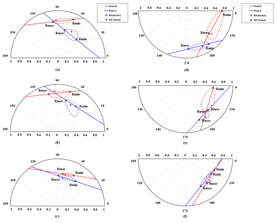
Figure 9.
Geometrical interpretation of pixels B and C for the three sizes from the Mabounie and Mondah areas: (a) 5 × 5 size from the Mabounie area; (b) 9 × 9 size from the Mabounie area; (c) 25 × 25 size from the Mabounie area; (d) 5 × 5 size from the Mondah area; (e) 11 × 11 size from the Mondah area; (f) 25 × 25 size from the Mondah area. Note that Rmax is the endpoint near the ground phase, Rmin is the endpoint away from the ground phase, and markers of different colors indicate the coherence amplitude at the HH channel under different sizes.
Similarly, pixels E and F were selected from ROI-II (see Figure 5) and the corresponding LiDAR forest heights are 2.55 m and 14.20 m, respectively. Numerically, for pixels E and F, the corresponding estimation errors are 52.44 m and 14.2 m for the 5 × 5 size, 48.77 m and 15.46 m for the 11 × 11 size, and 30.45 m and 25.23 m for the 25 × 25 size. From the numerical data and Figure 9d–f, we can also obtain the same conclusion as the Mabounie area. In the textured area, inversion accuracy benefits from a small multilooking size which avoids mixing multiple types of ground targets. Therefore, we can determine that large multilooking size causes the wrong selection of multiple heterogeneous pixels and the serious detail-blurring effect on the forest height image, which decreases the accuracy of forest height inversion.
In brief, through the analysis of geometric interpretations based on coherence region, we can determine that large multilooking size helps to reduce the statistical bias effect, and small multilooking size can prevent the accuracy of different forest height results being influenced by each other. Thus, a moderate multilooking size is suitable for PolInSAR forest height inversion.
4.3. Error Analysis Based on Statistical Indicators
We estimated the forest height results of both Mabounie and Mondah areas under the 5 × 5 to 25 × 25 multilooking sizes. Figure 10 and Figure 11 show the forest height inversion results of three multilooking sizes in Mabounie and Mondah, respectively. As the multilooking size increases, the image resolution decreases and the detail-blurring effect becomes more serious, indicating that a relatively small Boxcar filtering window size can effectively suppress imagery speckle noise while preserving the structure and textured features of different ground targets. This is due to the Boxcar filter averaging all sample pixels in the square window without any discrimination.
Figure 10.
Forest height inversion results for the three sizes in Mabounie: (a) 5 × 5 size; (b) 9 × 9 size; (c) 25 × 25 size.
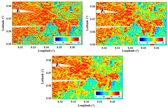
Figure 11.
Forest height inversion results for the three sizes in Mondah: (a) 5 × 5 size; (b) 11 × 11 size; (c) 25 × 25 size.
For a more intuitive accuracy assessment, we selected a total of 5840 forest stands and 2385 forest stands in a 50 × 50 window (100 m × 100 m) from the entire Mabounie and Mondah areas, respectively. For a forest stand , the estimation error of forest height can be calculated as:
where represents the forest height results of LiDAR. As shown in the estimation error histograms of the Mabounie and Mondah areas in Figure 12, there exists an overestimation problem in filtered results. Compared to the 5 × 5 size, the error distribution in larger sizes is more concentrated and also is closer to 0, especially in the Mabounie area. The overall curves in the 9 × 9 size are closer to 0, which means the bias is smaller.
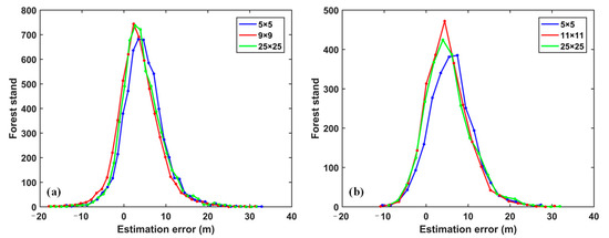
Figure 12.
Estimation error based on forest stands: (a) Mabounie; (b) Mondah.
To further quantitatively analyze height estimation performance for different multilooking sizes, the following equations are used to generate statistics for estimation errors of all forest stands using three statistical indicators, i.e., Root Mean Square Error (RMSE), Mean (MEAN), and Standard Deviation (STD). The three aforementioned evaluation indicators can be calculated based on the estimation error :
The RMSEs, MEANs, and STDs are calculated under different multilooking sizes for Mabounie (as shown in Figure 13a–c) and Mondah (as shown in Figure 13d–f). In the Mabounie area, it can be seen from Figure 13a–c that the RMSEs, MEANs, and STDs are consistent evaluation indicators in relation to changing trends. As size increases, the three statistical indicators first decrease and then increase and simultaneously achieve the smallest value in the 9 × 9 size. However, compared to the MEANs and RMSEs, the amplitude of variation for STDs is smaller, which explains how the performance of height estimation with different multilooking sizes is not so affected by STD and is seriously affected by bias. Specifically, compared with the maximum MEAN (5.40 m) and RMSE (6.75 m) corresponding to the 5 × 5 size, the MEAN (4.66 m) in the 9 × 9 size is reduced by 0.74 m, and the RMSE (6.07 m) in the 9 × 9 size is reduced by 0.68 m. Simultaneously, the difference between the maximum STD and minimum STD is only 0.2 m (from 4.10 m to 3.90 m for the 25 × 25 size and the 9 × 9 size, respectively).
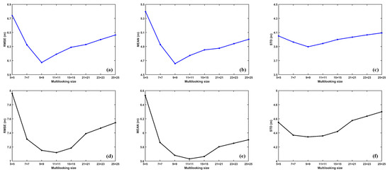
Figure 13.
Three statistical indicators based on estimation errors from the Mabounie and Mondah areas: (a) RMSE from the Mabounie area; (b) MEAN from the Mabounie area; (c) STD from the Mabounie area; (d) RMSE from the Mondah area; (e) MEAN from the Mondah area; (f) STD from the Mondah area.
In the Mondah area, the changes in MEAN, RMSE, and STD evaluation indicators are similar to the Mabounie area (see Figure 13d–f). Specific numerical comparison of the three statistical indicators shows that the MEAN (5.63 m) of the 11 × 11 size is 0.90 m less than the MEAN (6.53 m) of the 5 × 5 size, and the RMSE (7.12 m) of the 11 × 11 size is 0.84 m less than the RMSE (7.96 m) of the 5 × 5 size. The difference between the maximum STD and minimum STD is only 0.35 m (from 4.70 m to 4.35 m). This also explains that the RMSE is mainly affected by estimation bias under multiple multilooking sizes. Therefore, from the above statistical analysis of two different areas, we can determine that the accuracy of forest height inversion mainly depends on estimation bias rather than STD, indicating that an appropriate size can effectively reduce the estimation error.
4.4. Accuracy Analysis of Different Filtering Methods
To compare forest height inversion performance using different filtering methods we selected Boxcar filtering (optimal size of 9 × 9 in Mabounie, 11 × 11 in Mondah), refined Lee filtering [27] (11 × 11 edge-aligned neighborhood), and IDAN filtering [28] (adaptive neighborhood with maximum size of 50). The fixed extinction coefficient algorithm was also used with the same parameters as the above experiment for estimating forest height. Figure 14 shows forest height accuracy evaluation results for different filtering methods in the Mabounie and Mondah areas. It can be seen from Figure 14 that the MEAN, STD, and RMSE from refined Lee filtering are all the smallest, indicating that refined Lee filtering had the best-estimated result among the three filtering methods. In Mabounie, compared with Boxcar filtering and IDAN filtering, the RMSE of refined Lee filtering is increased by 7.4% and 9.9%, respectively. In Mondah, the RMSEs of the three filtering methods have a small difference, with refined Lee filtering only 0.18 m less than Boxcar filtering and 0.35 m less than IDAN filtering. This is because refined Lee filtering selects the optimal local template adaptively based on the edge-aligned gradient windows, and better distinguishes between pixels of different types of ground targets.
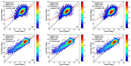
Figure 14.
The relationships between the LiDAR and PolInSAR heights for different filtering methods in the Mabounie and Mondah areas: (a) Boxcar filtering in the Mabounie area; (b) IDAN filtering in the Mabounie area; (c) refined Lee filtering in the Mabounie area; (d) Boxcar filtering in the Mondah area; (e) IDAN filtering in the Mondah area; (f) refined Lee filtering in the Mondah area.
5. Conclusions
In this paper, we used AfriSAR2016 SAR data sets including the Mabounie and Mondah areas to evaluate the performance of different multilooking sizes on single-baseline PolInSAR forest height inversion. Moreover, we also compared the forest height inversion performance using different filtering methods. Through this experiment, the main three contributions of our analysis work are as follows:
- (1)
- The pixel-wise detailed analysis based on the coherence set and scattering intensity reveals how multilooking size affects the tree height result. Polarimetric complex coherence is easily affected by the inherent speckle noise and finite multilooking effect, hence the coherent line segment degenerates into an ellipse which is biased by the ideal noise-free coherence region. Multilooking processing is an effective method which reduces speckle noise and the finite multilooking effect. Therefore, through analysis based on backscattering intensity and coherence region, we can determine that a large multilooking size helps to reduce the influence of statistical bias caused by the finite multilooking effect in homogeneous forest areas and a small multilooking size can prevent the influence of multilooking average without any discrimination. Thus, a moderate multilooking size is suitable for PolInSAR forest height inversion.
- (2)
- From the perspective of the overall error analysis, forest height inversion results mainly depend on estimation bias rather than estimation variance. Through statistics regarding estimation errors using three statistical indicators, we can determine that the accuracy of forest height inversion mainly depends on estimation bias rather than STD, indicating that an appropriate size can effectively reduce estimation error. Thus, the experimental result shows that the 9 × 9 size is the optimal one for the selected Mabounie area data set, and the 11 × 11 size is the optimal size in the Mondah area data set.
- (3)
- Three different filtering methods were compared, and refined Lee filtering is a more superior method. Comparing forest height inversion performance using different filtering methods, we found that refined Lee filtering had the best-estimated result because this filtering method selects the optimal local template adaptively based on the edge-aligned gradient windows and better distinguishes between pixels of different types of ground targets.
Thus, according to the estimated forest height results of different filtering methods, refined Lee filtering achieved the highest estimation accuracy. Therefore, this paper suggests selecting refined Lee filtering to reduce speckle noise and preserve detailed information in single-baseline PolInSAR forest height inversion processing.
Author Contributions
C.W. conceived the idea, performed the experiments, and wrote and revised the paper; C.H. performed the experiments, analyzed the experimental results, and revised the paper; P.S. contributed some ideas, analyzed the experimental results, and revised the paper; T.S. contributed to the discussion of the results. All authors have read and agreed to the published version of the manuscript.
Funding
This research was funded by the National Natural Science Foundation of China, grant number 42030112 and 41671356.
Institutional Review Board Statement
Not applicable.
Informed Consent Statement
Not applicable.
Data Availability Statement
The data presented in this study was obtained from the European Space Agency Earth Observation Campaigns Data Project and are available with the permission of the ESA.
Acknowledgments
The authors would like to thank the German Aerospace Center (DLR) and the National Aeronautics and Space Administration (NASA) for providing the AfriSAR 2016 campaign multibaseline polarimetric synthetic aperture radar interferometry (PolInSAR) data and Land, Vegetation, and Ice Sensor (LVIS) light detection and ranging (LiDAR) data of the test site.
Conflicts of Interest
The authors declare no conflict of interest.
References
- Bonan, G.B. Forests and climate change: Forcings, feedbacks, and the climate benefits of forests. Science 2008, 320, 1444–1449. [Google Scholar] [CrossRef] [PubMed] [Green Version]
- Cloude, S.R. Polarimetric SAR interferometry. IEEE Trans. Geosci. Remote Sens. 1998, 99, 1551–1565. [Google Scholar] [CrossRef]
- Neumann, M.; Ferro-Famil, L.; Reigber, A. Estimation of forest structure, ground, and canopy layer characteristics from multibaseline polarimetric interferometric SAR data. IEEE Trans. Geosci. Remote Sens. 2010, 48, 1086–1104. [Google Scholar] [CrossRef] [Green Version]
- Wang, C.; Wang, L.; Fu, H.; Xie, Q.; Zhu, J. The impact of forest density on forest height inversion modeling from polarimetric InSAR data. Remote Sens. 2016, 8, 291. [Google Scholar] [CrossRef] [Green Version]
- Fu, H.; Wang, C.; Zhu, J.; Xie, Q.; Zhang, B. Estimation of pine forest height and underlying dem using multi-baseline P-band PolInSAR data. Remote Sens. 2017, 9, 363. [Google Scholar] [CrossRef] [Green Version]
- Treuhaft, R.N.; Siqueira, P.R. Vegetation characteristics and underlying topography from interferometric radar. Radio Sci. 2000, 35, 141–177. [Google Scholar] [CrossRef] [Green Version]
- Ballester-Berman, J.D.; Lopez-Sanchez, J.M. Combination of direct and double-bounce ground responses in the homogeneous oriented volume over ground model. IEEE Geosci. Remote Sens. Lett. 2011, 8, 54–58. [Google Scholar] [CrossRef]
- Cloude, S.R. Polarization coherence tomography. Radio Sci. 2006, 41, RS4017. [Google Scholar] [CrossRef]
- Zhang, H.; Ma, P.; Wang, C. A new function expansion for polarization coherence tomography. IEEE Geosci. Remote Sens. Lett. 2012, 9, 891–895. [Google Scholar] [CrossRef]
- Lombardini, F.; Reigber, A. Adaptive spectral estimation for multi baseline SAR tomography with airborne L-band data. In Proceedings of the 2003 IEEE International Geoscience and Remote Sensing Symposium (IGARSS), Toulouse, France, 21–25 July 2003. [Google Scholar] [CrossRef]
- Cazcarra-Bes, V.; Tello-Alonso, M.; Fischer, R.; Heym, M.; Papathanassiou, K. Monitoring of forest structure dynamics by means of L-band SAR tomography. Remote Sens. 2017, 9, 1229. [Google Scholar] [CrossRef] [Green Version]
- Lavalle, M.; Simard, M.; Pottier, E.; Solimini, D. PolInSAR forestry applications improved by modeling height-dependent temporal decorrelation. In Proceedings of the 2010 IEEE International Geoscience and Remote Sensing Symposium (IGARSS), Honolulu, HI, USA, 25–30 July 2010. [Google Scholar] [CrossRef]
- Zhang, B.; Fu, H.; Zhu, J.; Peng, X.; Lin, D.; Xie, Q.; Hu, J. Forest height estimation using multibaseline low-frequency PolInSAR data affected by temporal decorrelation. IEEE Geosci. Remote Sens. Lett. 2022, 19, 1–5. [Google Scholar] [CrossRef]
- Managhebi, T.; Maghsoudi, Y.; Zoej, M.J.V. Four-stage inversion algorithm for forest height estimation using repeat pass polarimetric SAR interferometry data. Remote Sens. 2018, 10, 1174. [Google Scholar] [CrossRef] [Green Version]
- Papathanassiou, K.P.; Cloude, S.R. The effect of temporal decorrelation on the inversion of forest parameters from Polinsar data. In Proceedings of the 2003 IEEE International Geoscience and Remote Sensing Symposium (IGARSS), Toulouse, France, 21–25 July 2003. [Google Scholar] [CrossRef]
- Lavalle, M.; Hensley, S. Extraction of structural and dynamic properties of forests from polarimetric-interferometric SAR data affected by temporal decorrelation. IEEE Trans. Geosci. Remote Sens. 2015, 53, 4752–4767. [Google Scholar] [CrossRef]
- Ghasemi, N.; Tolpekin, V.; Stein, A. A modified model for estimating tree height from PolInSAR with compensation for temporal decorrelation. Int. J. Appl. Earth Obs. Geoinf. 2018, 73, 313–322. [Google Scholar] [CrossRef]
- Lu, H.; Suo, Z.; Guo, R.; Bao, Z. S-RVoG model for forest parameters inversion over underlying topography. Electron. Lett. 2013, 49, 618–620. [Google Scholar] [CrossRef]
- Garestier, F.; Toan, T. Le Forest modeling for height inversion using single-baseline InSAR/Pol-InSAR data. IEEE Trans. Geosci. Remote Sens. 2010, 48, 1528–1539. [Google Scholar] [CrossRef]
- Papathanassiou, K.P.; Cloude, S.R. Single-baseline polarimetric SAR interferometry. IEEE Trans. Geosci. Remote Sens. 2001, 39, 2352–2363. [Google Scholar] [CrossRef] [Green Version]
- Cloude, S.R.; Papathanassiou, K.P. Three-stage inversion process for polarimetric SAR interferometry. IEE Proc. Radar Sonar Navig. 2003, 150, 125–134. [Google Scholar] [CrossRef] [Green Version]
- Dubois-Fernandez, P.C.; Souyris, J.C.; Angelliaume, S.; Garestier, F. The compact polarimetry alternative for spaceborne SAR at low frequency. IEEE Trans. Geosci. Remote Sens. 2008, 46, 3208–3222. [Google Scholar] [CrossRef]
- Garestier, F.; Dubois-Fernandez, P.C.; Champion, I. Forest height inversion using high-resolution P-band PoI-InSAR data. IEEE Trans. Geosci. Remote Sens. 2008, 46, 3544–3559. [Google Scholar] [CrossRef]
- Zhu, J.; Xie, Q.; Zuo, T.; Wang, C.; Xie, J. Criterion of complex least squares adjustment and its application in tree height inversion with PolInSAR data. Acta Geod. Cartogr. Sin. 2014, 43, 45–51. [Google Scholar] [CrossRef]
- Shen, P.; Wang, C.; Hu, J.; Fu, H.; Zhu, J. Interferometric phase optimization based on PolInSAR total power coherency matrix construction and joint polarization-space nonlocal estimation. IEEE Trans. Geosci. Remote Sens. 2022, 60, 1–14. [Google Scholar] [CrossRef]
- Tabb, M.; Flynn, T.; Carande, R. Estimation and removal of SNR and scattering degeneracy effects from the PolInSAR coherence region. In Proceedings of the 2003 IEEE International Geoscience and Remote Sensing Symposium (IGARSS), Toulouse, France, 21–25 July 2003. [Google Scholar] [CrossRef]
- Lee, J.S.; Cloude, S.R.; Papathanassiou, K.P.; Grunes, M.R.; Woodhouse, I.H. Speckle filtering and coherence estimation of polarimetric SAR interferometry data for forest applications. IEEE Trans. Geosci. Remote Sens. 2003, 41, 2254–2263. [Google Scholar] [CrossRef]
- Vasile, G.; Trouvé, E.; Buzuloiu, V. Intensity-driven adaptive-neighborhood technique for polarimetric and interferometric SAR parameters estimation. IEEE Trans. Geosci. Remote Sens. 2006, 44, 1609–1620. [Google Scholar] [CrossRef] [Green Version]
- Lee, J.S.; Pottier, E. Polarimetric Radar Imaging: From Basics to Applications; CRC Press: Boca Raton, FL, USA, 2009. [Google Scholar]
- Lüneburg, E.; Ziegler, V.; Schroth, A.; Tragl, K. Polarimetric Covariance Matrix Analysis of Random Radar Targets. Target and Clutter Scattering and Their Effects on Military Radar Performance. 1997. Available online: https://apps.dtic.mil/sti/pdfs/ADA244893.pdf#page=250 (accessed on 10 April 2022).
- Tabb, M.; Orrey, J.; Flynn, T.; Carande, R. Phase diversity: A decomposition for vegetation parameter estimation using polarimetric SAR interferometry. Proc. EUSAR 2002, 2, 721–724. [Google Scholar]
- Hajnsek, I. Technical Assistance for the Development of Airborne SAR and Geophysical Measurements during the AfriSAR Campaign; ESA: Paris, France, 2011. [Google Scholar]
- Kugler, F.; Lee, S.K.; Hajnsek, I.; Papathanassiou, K.P. Forest Height Estimation by Means of Pol-InSAR Data Inversion: The Role of the Vertical Wavenumber. IEEE Trans. Geosci. Remote Sens. 2015, 53, 5294–5311. [Google Scholar] [CrossRef]
- Flynn, T.; Tabb, M.; Carande, R. Coherence region shape extraction for vegetation parameter estimation in polarimetric SAR interferometry. In Proceedings of the 2002 IEEE International Geoscience and Remote Sensing Symposium (IGARSS), Toronto, ON, Canada, 24–28 June 2002. [Google Scholar]
Publisher’s Note: MDPI stays neutral with regard to jurisdictional claims in published maps and institutional affiliations. |
© 2022 by the authors. Licensee MDPI, Basel, Switzerland. This article is an open access article distributed under the terms and conditions of the Creative Commons Attribution (CC BY) license (https://creativecommons.org/licenses/by/4.0/).