Abstract
An agreement between the provincial government of Québec, Canada and the forest industry executing forest management activities on public lands has been established regarding non-utilized woody material (NUWM) left on the cutting area. Problems linked to this agreement are compounded by labor shortages, which have an impact on the precision of the mandatory inventories. The objectives of this study were to: (1) reconstruct and estimate the merchantable NUWM volume beyond the last processed log of balsam fir and white spruce with the use of harvester on-board computer (OBC) data, (2) design a software tool to estimate and spatialize merchantable NUWM, and (3) perform an explorative comparison between the OBC method and conventional field inventory. In total, five sites were harvested to develop the volume algorithms. Each site was harvested by a single-grip harvester operating a different OBC system (OPTI4G, Log Mate 500, and Log Mate 510). Results suggest that, with Varjo’s model and linear regression, estimation of NUWM volume using OBC data is possible. The spatialization tool positioned NUWM within the harvest area for StanForD and StanForD 2010. The explorative comparison highlighted a possible cost reduction of approx. 36.8 $/ha and an increase of precision for the OBC method.
1. Introduction
Forest operations create harvesting residues in the form of woody debris, branches, tree-tops, and foliage. The amount and spatial distribution of these residues depend on the stand, silvicultural treatment, and harvesting method [1]. Two harvesting methods are predominant in eastern Canada: full tree (FT) and cut-to-length (CTL). In FT operations, trees are felled and extracted from the stand, while processing, the task of delimbing and cross-cutting a stem into different assortments, occurs at a landing area. During CTL operations, the felling and processing tasks are done directly in the stand [2,3]. When the extraction of biomass for bioenergy is not required, these two harvesting methods create different harvesting residue distribution patterns. In the CTL method, residues remain in the stand whereas they are accumulated at landings or processing areas in the FT method. Often, the main stem can have residues with a merchantable diameter. These normally occur when a harvester is not able to create another product with the remaining portion of the tree, while considering merchantable assortments of the region.
As forest management in Québec, Canada, aspires to achieve sustainable forest management on public lands [4], an agreement between the provincial government and the forest industry carrying out forest management activities has been established regarding the merchantable timber left on the cutting area. This agreement comes with the obligation to perform a field inventory after harvesting activities. In the province of Québec, the merchantable section of a harvesting debris is called non-utilized woody material (NUWM). A NUWM is defined as “all usable ligneous material from felled trees or parts of commercial species trees left on the cutting area” and the smallest diameter considered as merchantable is 9.1 cm [5]. The goal of the agreement is to monitor the amount of NUWM left after harvesting operations. With the information, there are certain regional variations in terms of what is the upper limit of acceptable NUWM volume. This limit is a function of the species being harvested and their proximity to wood processing facilities. When the transportation distance between a harvest site and a processing facility is too far, the regional agreement allows for a higher volume of NUWM to be left on the harvest site.
Problems linked to this agreement are currently compounded by issues of labor shortages [6], which have a direct impact on the precision of the inventories when the required frequency of transects cannot be maintained. In addition, the amount of NUWM is currently being monitored via expensive field inventories (approx. 50$/ha) performed after harvesting operations. Moreover, the Gaspésie region of Québec (Figure 1) faces unique circumstances influencing the forest dynamics of the region. The geographical position of the region makes it isolated resulting in long transportation distances to wood processing facilities, especially for pulpwood products. Furthermore, this region is faced with a decrease in demand for pulpwood (softwood, hardwood, and poplar). Despite the presence of two processing plants requiring chips of hardwood and poplar, the associated supply costs are particularly high due to the remoteness of raw materials. Faced with these conflicting issues, the Québec Ministry of Forests, Wildlife, and Parks (MFFP) and local industrial stakeholders are seeking alternatives to conventional NUWM field inventories. One of the alternatives being considered is the use of harvester data.

Figure 1.
(a) General location of the targeted Gaspésie region of Québec, Canada; (b) Location of the five harvest areas; (c) Close-up of a harvest area and study area.
Modern harvesters, as used in CTL mechanized operations, record length, diameter, and volume of every processed log [7]. This information is stored and classified into reports, and those are standard for each harvester [8]. The Standard for Forest machine Data and Communication (StanForD) was developed in the late 80’s by Skogforsk and is used internationally on most harvester on-board computers (OBC) [8]. Two standards are currently used in Canada, StanForD and StanForD 2010. The new standard works in an open .xml format and is easily readable without special and expensive software. Moreover, many changes occurred in the file types, whereas StanForD 2010 added the notion of time scale, which was not available in the previous version [9].
In many regions, the usefulness of OBC data remains marginal in forest operations primarily concerning the accuracy and integrity of real-time data [10]. Thus far, OBC data have most frequently been used for bucking optimization and for productivity studies [2,11,12]. The use of OBC data for topics of inventory and improvement of operation management is less frequent [7]. Beyond the collection and analysis of physical parameters, OBC data can be used to estimate harvester utilization rates and to accurately calculate machine hourly costs [7,11]. Studies have shown that through OBC data, it is possible to estimate the biomass of individual trees left on site [8,12]. Specifically, a tool was developed to assess the residual biomass of Eucalyptus sp. (L’Hér., 1789) based on OBC data collected from individually harvested trees [13]. The tool used a linear model by including tree dependent variables such as diameter, height, and the combination of the two. Results provided the residual Eucalyptus biomass in real-time. To improve the model, Rodrigues (2019) suggested consideration of age, species, genetics, and growth of the trees as important characteristics [13]. In another study, the height of individual trees was effectively reconstructed using log data from CTL harvesters used in a radiata pine (Pinus radiata) plantation [14,15]. In all study cases above, the aim was to evaluate non-utilized woody material and no differentiation was made between merchantable or non-merchantable volumes. The agreement between MFFP and stakeholders only applies to the merchantable section of the tree (greater than 9.1 cm diameter).
Considering the significant labor shortage and the reduction in profit margins for private companies, the aim of this project was to estimate the volume of merchantable NUWM after mechanized CTL harvesting operations using OBC data.
The following objectives were addressed:
- (1)
- Develop mathematical functions to reconstruct and estimate the section of merchantable NUWM of balsam fir (Abies balsamea L. (Mill)) and white spruce (Picea glauca (Moench) Voss), beyond the last processed log, using on-board computer data.
- (2)
- Design a software tool to estimate and spatialize the volume of merchantable NUWM for the two target species.
- (3)
- Perform an explorative comparison of the technical and economic performance between the forecasts of the NUWM volume obtained with OBC data and conventional NUWM field inventory.
2. Materials and Methods
2.1. Site Description and Experimental Design
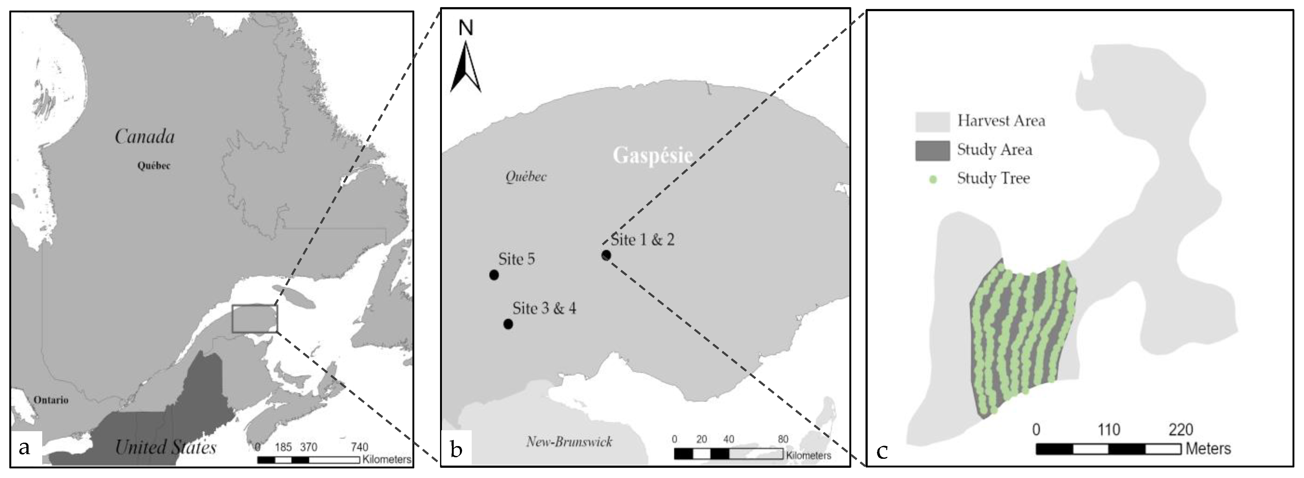
The study was conducted in the Gaspésie region in the province of Québec, Canada (48°40′00″ N, 65°40′00″ W; Figure 1a). The region is bordered by the St. Lawrence River to the north, the Gulf of St. Lawrence to the east, and Chaleur Bay to the southeast. Focus was set on two native tree species of Québec: balsam fir and white spruce. Both species represent 70% of the coniferous volume in the Gaspésie region [16].
In total, five harvest areas (Figure 1b; Table 1) were used for the design of the volume algorithms and met these three criteria: (1) an area from 5 to 15 ha, (2) harvest volume between 1000 and 1500 m3 of white spruce and balsam fir, and (3) homogeneity in terms of composition and topography. A variable radius inventory with a prism basal area factor 2 was carried out to allow the selection of the harvest area within the harvest calendar of the Gaspésie forest industry. Sampling frequency was set at 1 plot/3 ha for harvest sites smaller than 10 ha and 1 plot/5 ha for sites larger than 10 ha. Selected harvest areas were in natural and mature forests. A study area was randomly assigned to each harvest area. It was not the intention to have a fixed area dedicated as study area but rather allow the selection of at least 100 white spruce and 100 balsam fir trees (Figure 1c).

Table 1.
Site composition of the five harvest areas including mean DBH, height and volume of the five study sites. Statistical differences (aov function) based on Tukey test (Tukey HSD function) between study area characteristics are illustrated in parentheses.
To select appropriate harvesters, a survey was prepared and circulated to all forest entrepreneurs using CTL harvesters in the Gaspésie region. The goal was to populate a list of harvesters, harvesting heads, and OBC systems being used. Based on the collected data, five harvesters were selected to harvest one harvest area each; three Ponsse with the OPTI4G on-board system and two Log Max, one under Log Mate 500 and the other under Log Mate 510 on-board system. (Table 2). Three of the selected harvesters were using StanForD and two were on StanForD 2010.
Table 2.
Harvester, harvesting head, and on-board computer specifications.
2.2. Pre-Harvest Inventory
In each study area, a unique alphanumeric code was painted to identify study trees. Red was used for white spruce (Figure 2a) and yellow for balsam fir (Figure 2b). Species, diameter at breast height (breast height = 1.3 m) (obtained by averaging two perpendicular diameter measurements (1 mm accuracy)), and tree height recorded at 0.5 m accuracy with a digital height, distance, and inclination instrument (Vertex IV and Transponder T3) were recorded.
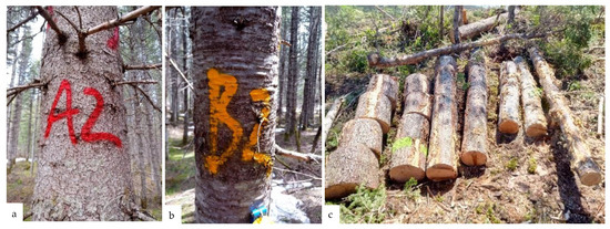
Figure 2.
Example of alphanumeric code painted on study trees (a) White Spruce (b) Balsam fir; (c) Example of stem reconstruction.
Since machine operating trails were not planned before harvesting, the unique alphanumeric code was painted on four sides of the study trees at 0.2 m and 2 m in height to ensure visibility in video footage. A binary code was used to characterize tree form. For assessment, a study tree was divided into three merchantable sections of approximately the same length, and if there was a complex geometry for a respective section, a code of 1 was tallied and a code of 0 was tallied if the section did not present any issues that would hinder harvesting productivity. For example: a stem with only a fork at the last section would receive a code of 0-0-1 [17].
2.3. Machine Specifications and Operating Procedure
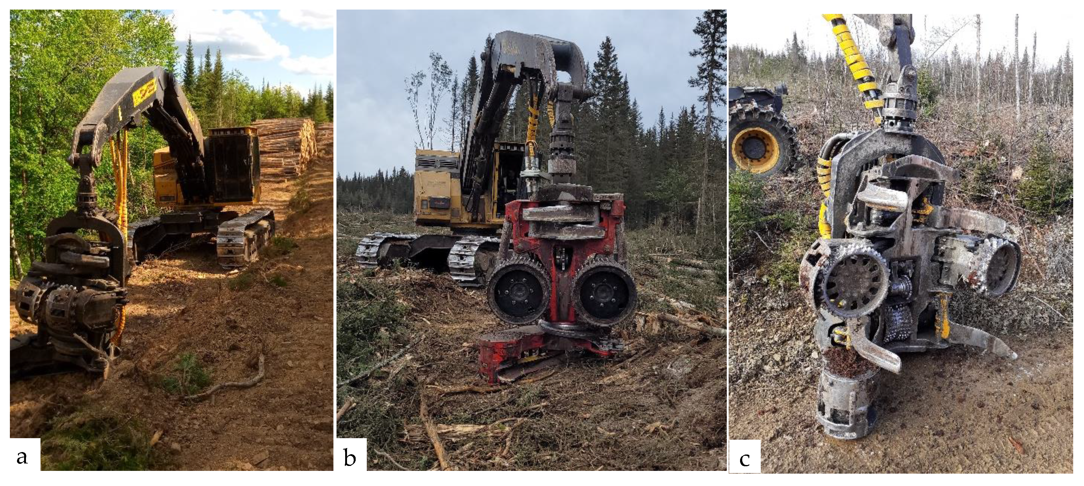
Each of the five harvesters were calibrated as prescribed by the manufacturer (Figure 3). A project was created in the OBC to gather data (production and GPS tracking) of all study trees. Operators were instructed to first harvest unmarked trees and to transport the logs to the side of the road before starting to harvest the study trees. This sequence was applied to avoid confusion during the field inventory. Woody material derived from individual study trees (products, discs, forks, and tops) was laid on the ground to facilitate measurements and reconstruction within the database (Figure 2c).

Figure 3.
Harvesting heads used in the study, (a) Ponsse H8HD; (b) LogMax6000V; (c) Ponsse H7.
Video footage was obtained by two digital video cameras (GoPro) mounted inside the harvester cabin. One camera was aimed at the harvesting head while the other was directed at the OBC screen. Time-sensitive video footage of both cameras was used to pair field data with OBC data. Data concerning the length, diameter, and volume per log was acquired through .hpr/.pri and compiled by the harvesters OBC.
2.4. Post-Harvest Inventory
After harvesting, post-inventory was carried out on the minimum 200 study trees. For every tree, the length of each harvested section was measured with a measuring tape (cm accuracy). Two perpendicular diameter measurements (1 mm accuracy) were taken for the small- and large-end diameters of each harvested section of the tree (Figure 2c). Every section of the stem was sequentially numbered to facilitate its reconstruction.
2.5. Data Analysis
Data were first verified for ANOVA prerequisites, homoscedasticity, and normality. Through an ANOVA and a Tukey test, characteristics of study trees (DBH, height, and gross merchantable volume) were than evaluated to verify if any statistical difference existed between study sites [18]. Gross merchantable volume was calculated using Perron’s cubing rate [19]. All statistical analyses, ANOVA’s, Tukey tests, and linear regressions were performed using R 4.1.2 (1 November 2021) (Ihaka, R. and Gentleman, R. (1993) Auckland, New-Zealand), and the underlying significance level used in all tests was 5%. The following sections presents the stepwise approach used for data analysis to achieve the first objective.
2.5.1. Stem Reconstruction
The first step was to reconstruct the stem in the OBC data. In some cases, when the tree presented a complex geometry (such as forks, sweeps, and crooks) the feed-rollers and associated delimbing knives of the harvesting head needed to be opened/repositioned to allow bypassing a portion of a stem. In this instance, a new tree count was triggered in the OBC data despite being the same tree as compared to the pre-bypassed section. To eliminate this problem, a combination of data sources was used to find and evaluate the occurrences. The first data source was a compilation of the inventoried characteristics of the tree before harvesting. The second dataset was the production file of the OBC and .hpr/.pri, whereas the third dataset was taper measurement of the logs manually recorded after harvesting.
Video footage of all harvesting activities within the study area was evaluated to associate OBC and field data on a per tree level. Within the pre-harvest inventory, some tree breaks (log or top) were observed and omitted from the study since their reconstruction was not possible. Moreover, trees were also omitted when the association between OBC data and field data was impossible, mainly due to camera issue or with difficulties in identifying the alphanumeric number.
OBC data and field data were then merged in Microsoft Excel to create a master file by harvest area. An exploratory analysis was performed to compare and validate the precision between OBC data and field data using the aov function from stats package (3.6.2) [18].
2.5.2. Estimation of Total Tree Length above Stump Height
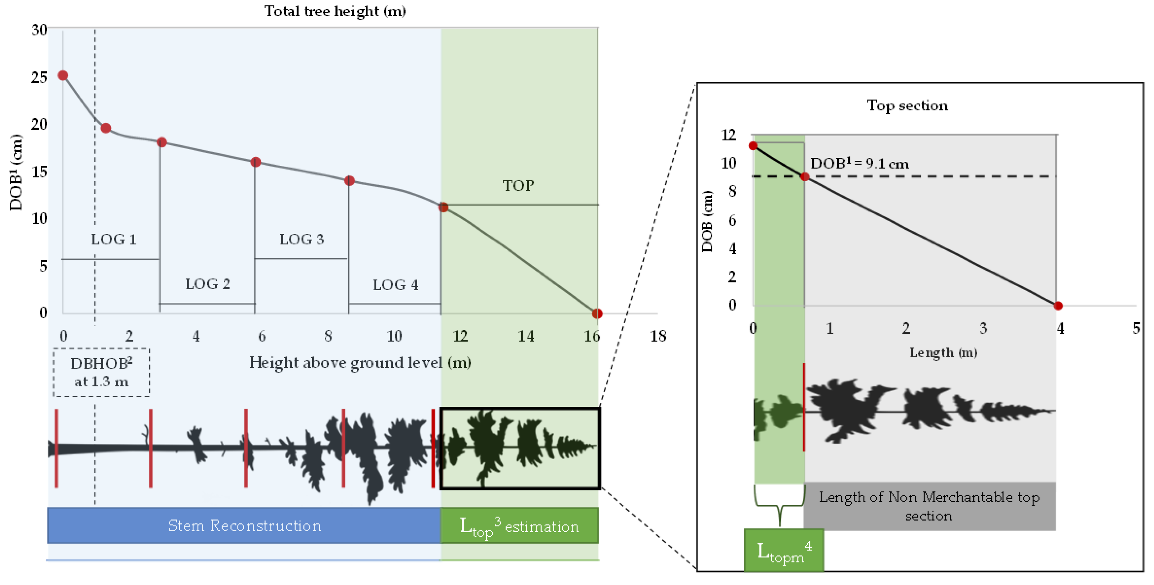
To estimate the merchantable top section of a tree, multiple analyses were done, and the most accurate response was obtained by first estimating total tree length above stump. The stepwise approach to estimate total tree length above stump is described in the following section (Figure 4).

Figure 4.
Reconstruction and estimation of top length, total length, and merchantable top length 1 DOB: Diameter over bark; 2 DBHOB: Diameter at breast height over bark; 3 Ltop: Top length; 4 Ltopm: (Merchantable top length).
Varjo (1995) formulated a model to predict the length of the top section of a tree that is not processed by the harvesting head for pine, spruce, and birch species in Finland. The model developed uses total log length, diameter at breast height over bark (DBHOB), and the small-end diameter under bark of the last log (SEDUB) [20]. Afterwards, Lu et al. modified Varjo’s model, by replacing SEDUB by small-end diameter over bark (SEDOB), to use in a radiata pine plantation [14].
We also used Varjo’s modified model to estimate total tree length above stump for balsam fir, since no model was made for this species.
- Ltop: top section length (m)
- L: total log length (m)
- DBHOB: diameter at breast height over bark (cm)
- SEDOBTL: small-end diameter over bark of the last log (cm)
- ax: parameter
The species dependent database was divided randomly to use 75% of the data to estimate parameters and 25% to test the model. Parameters were estimated through linear regression (lm function), with the stats package (3.6.2) [18]. Outlier analysis of the difference between observed and predicted was performed with Rosner’s test in EnvStats package (version 2.3.1) (Steven P. Millard, Seattle, United States of America) [21]. Homoscedasticity and normality were tested using standard graphical procedures. Observed values were obtained by subtracting total log length and an average stump height of 0.15 cm from the total height measured with a digital height, distance, and inclination instrument (Vertex IV and Transponder T3). Residuals were examined by using both diagnostic plots and statistical tests to detect possible violations of the normality assumption. To correct for log transformation bias, Snowdon’s (1991) bias correction factor was calculated following parameter estimation.
Using the estimated Ltop, the predicted total tree height above stump height was calculated using Varjo’s modified model. The model is generally used to estimate total tree height through the addition of stump height, total length and back transformed predicted Ltop. In this study, stump height was excluded from Equation (2) (modified Varjo’s model) since the objective was to estimate total length above stump level, rather than total height of the tree including its stump.
- H: total tree length above stump level (m)
- L: total log length (m)
- θ: Snowdon’s bias correction factor
Logarithmic regression in the system of equations created bias in the estimation of total tree length above stump level when the predicted values were back-transformed from logarithm. To correct this bias, Snowdon’s bias correction factor, the ratio of the arithmetic sample mean and the mean of the back-transformed predicted values from the regression, was calculated [22]. lnLtop is the predicted value of log transformed Ltop from Equation (1) to evaluate the predictive performance of Equation (2). Using the observed and converted values of H, the mean error of prediction (MEP), mean absolute error of prediction (MAEP), mean squared error of prediction (MSEP) and the prediction coefficient of determination (R2p) were calculated. Four benchmarking statistics (Equations (3)–(6)), commonly used to assess predictive performance of forest models were used to evaluate the predictive results [14,23].
- Hp∶ predicted values
- Ho∶ observed values
- ∶ average of the observe values Ho
- n∶ number of samples in validation data
Among the validation statistics, MEP indicates the direction of the differences between observed and predicted values. The MAEP removes the signs of the prediction errors and gives the absolute differences between observed values and predicted values, whereas R2p reports the model’s efficiency coefficient. MEP and MAEP give an indicator to the accuracy of the model’s prediction, while MSEP and R2p describe its precision [14].
2.5.3. Estimating Merchantable Tree-Top
Stem reconstruction and predicted total tree height were used to estimate the merchantable section of the tree-top (Figure 4). Species dependent databases were used to compare predicted vs observed values. To validate the estimation of merchantable tree-tops, several methodological approaches were tested, and their results were compared with each other. The most accurate in terms of precision and coherent response was a linear regression model, developed for each individual tree using the last log and the estimated total length. Parameters a and b were estimated individually for each tree, to allow the best fit possible, using small-end diameter and sum of log length in .hpr/.pri report.
- Ltopm: length of the merchantable top section (m)
- DOBM: diameter over bark merchantable (cm) and equal 9.1 cm
- a and b: estimated parameters
Predicted value was compared to merchantable length measured in the field. Trees that did not have the measured length of top at 9.1 cm, because of breakage of the tree-top were omitted from the database. Moreover, trees for which the last log had a diameter equal or smaller to 9.1 cm were excluded, since by default their top could not have merchantable timber. The same four benchmarking statistics were used (Equations (3)–(6)) as total tree height.
2.6. Software Tool
The software tool was developed with WinForm ×64 as an interface in. NET with the collaboration of FORAC Research Consortium (Québec City, QC, Canada). The main objective was to spatialize the NUWM for every harvest site. An editable matrix was created to separate processed logs from NUWM. This matrix can be modified and tailored to individual stakeholder needs (i.e., product 1: length of 500 ± 5 cm and small-end diameter of 9.1 cm). Other logs in. pri/hpr files that do not match the assortments in the matrix are considered as NUWM. It was developed considering the difference of StanForD and StanForD 2010.
Volume calculation is done by using the same algorithms that are selected in the harvester and the estimated top length will be used to calculate, with the same algorithms, the volume of the top section. Symbology was created to attribute a color code; color gradient from green to red, starting at 0 m3/ha in 5 m3/ha increments, until the maximum value is reached.
Both .hpr and .pri files (StanforD 2010 and StanForD) can be used as input with GPS tracklog. The execution of the software tool provides the spatialization of NUWM in shapefile format. With a .pri file, it is possible to obtain positioning of the stem if the harvesting head is equipped with a GPS sensor [24]. However, this was not the case in our project. This mean that it is not possible to have information on time of harvest by stem in the pri file. Therefore, standard GPS are installed in the cabin of the harvester as standard equipment. Considering these facts, the version of the software tool is more primitive and only located the harvester by using the date of GPS tracklog and the start and end date of the project. A volume by hectare is calculated using the total volume of the stem in the harvest area and the area in hectares. With .hpr files and their integrated timestamps, every stem was positioned combining GPS track log and .hpr. A 100 m × 100 m (1 ha) fishnet is performed by the tool and the addition of the NUWM volume per hectare is represented in every square of the fishnet grid.
2.7. Assessment and Comparision
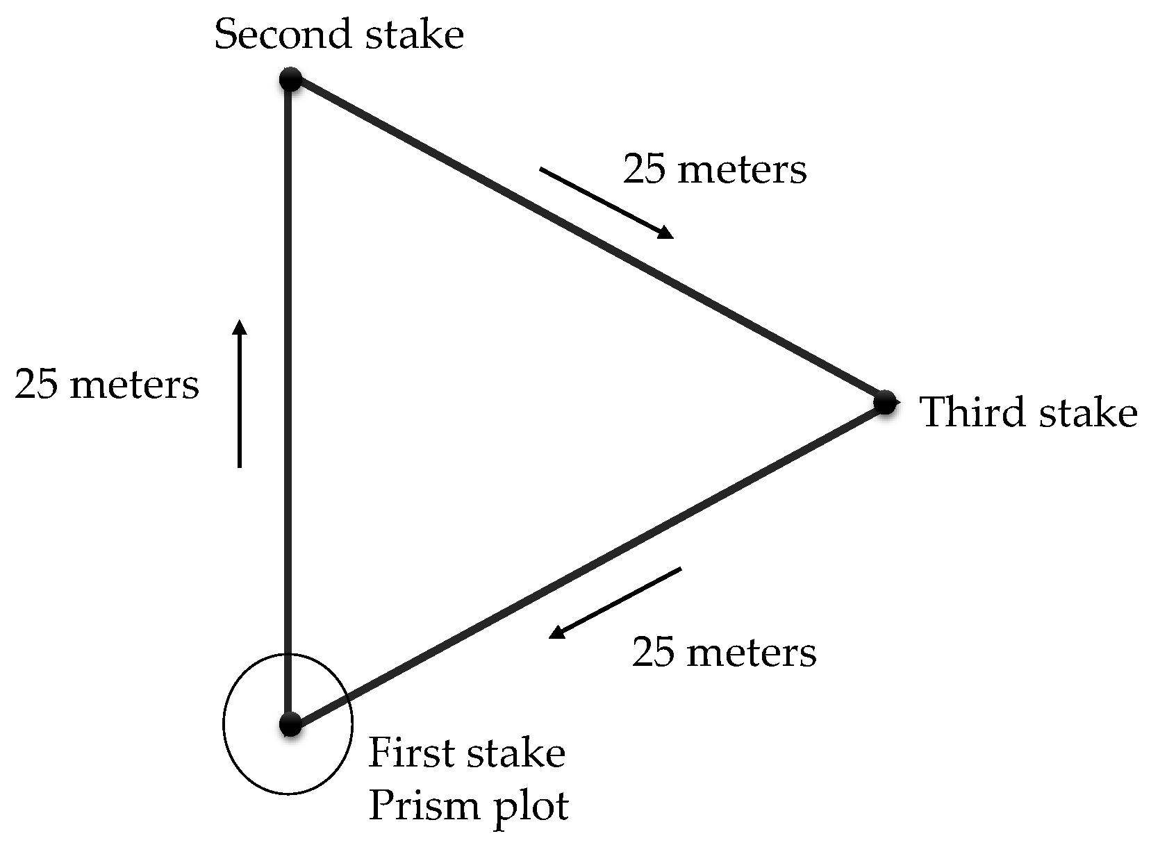
Conventional NUWM field inventory in Gaspésie region is based on an equilateral triangular transect method, where three stakes are set 25 m apart [25]. With this method, a variable radius plot is performed at the first stake. In the variable radius plot, only merchantable standing trees are evaluated and species, DBH and total height are noted. In the transect method, only merchantable debris resulting from harvesting activities are considered. Between each stake, each merchantable debris that crosses the 25-m line has its small- and large-end diameters and length measured (Figure 5). NUWM inventory sampling is forest type sensitive and requires a minimum of transect plots considering the harvested area by forest type. Sampling frequency varies between 15 plots for areas smaller than 20 ha to 70 plots for areas larger than 250 ha. If the transect plot minimum is respected, there is no requirement to have a plot in each harvest area of a forest block. A literature review was made, and our expert knowledge was used to orient the explorative comparison. A summary table was made to facilitate the understating of the exploratory comparison.

Figure 5.
Schematic reconstitution of conventional NUWM triangular transect.
3. Results
3.1. Pre-Harvest Study Tree Inventory
A total of 974 study trees were used to develop the algorithms. Sample size per site varied between 70 and 103 for white spruce and between 95 and 122 for balsam fir. DBH varied between 20.1 and 25.1 cm for white spruce and between 19.6 and 21.3 cm for balsam fir. No significant difference for DBH was observed between the five sites for balsam fir in contrary to white spruce, where a statistical difference occurred between the sites. The height of white spruce trees ranged from 12.9 to 17.3 m, whereas balsam fir oscillated between 14.3 and 16.5 m. Gross merchantable volume per tree varied between 0.19 and 0.39 m3 for white spruce and between 0.19 and 0.26 m3 for balsam fir with statistical differences detected between all five sites (Table 3).
Table 3.
Characteristics of study trees by study area. Statistical differences (aov function) based on Tukey test (Tukey HSD function) are illustrated in parentheses and are species dependent.
3.2. Estimating Total Tree Height
Before evaluating the possibilities of estimating total tree height, sum of length, small-end diameter by log and DBH were tested with an ANOVA and a Tukey test and no significant difference was detected.
For white spruce, 355 trees were used to estimate the parameters and 105 for testing (Table 4; Figure 6). The estimated parameters a1, a3 and a6 for white spruce were significantly different from zero. Since the prediction of the model was not improved by the removal of the other parameters, we decided to keep all parameters, as in Varjo’s model. The model explained 40.6% of the variation in the log transformed Ltop and the calculated bias correction factor was 0.985.
Table 4.
Parameter estimates, along with their standard errors in brackets and Snowdon’s bias correction factor (h) for Varjo’s model in Equation (1) for white spruce and balsam fir.
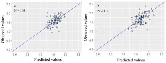
Figure 6.
Observed lnLtop plotted against predicted values with a line of unity for (a) white spruce and (b) balsam fir.
For balsam fir, 390 trees were used to estimate the parameters and 120 for testing (Table 4; Figure 6). The estimated balsam fir parameters a5 and a6 were significantly different from zero. The model explained 47.5% of the variation in the log transformed Ltop. The calculated bias correction factor was 0.994. Following Rosner’s outlier test, only one outlier was found in the balsam fir dataset where height was less than the length of the log and this sample was excluded.
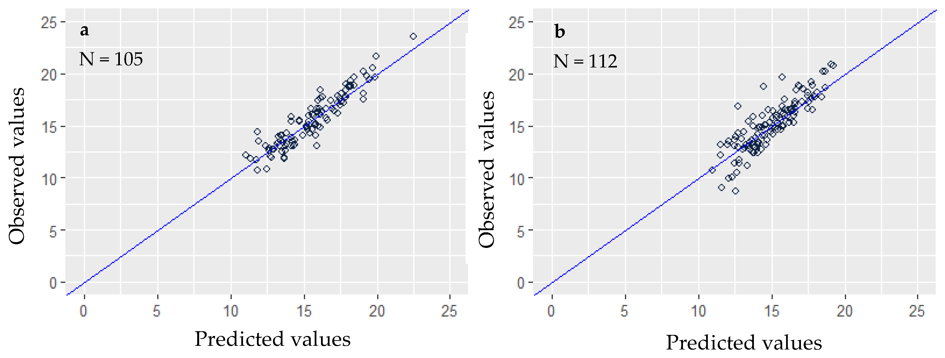
The predicted lnLtop was back-transformed from logarithm, corrected for log-transformation bias, and included in Equation (2) for the prediction of total tree length above stump (Figure 7). Bias in white spruce prediction of total tree length above stump (MEP) was −0.0069 m and the average size of the prediction error was 0.1757 m (MAEP). The value of MSEP was 0.2058 and the prediction coefficient of determination was 0.8603. Bias in balsam fir prediction of total tree length above stump (MEP) was 0.0958 m and the average size of the prediction error was 0.9539 m (MAEP). The value of MSEP was 1.6079 and the prediction coefficient of determination was 0.7312.
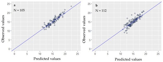
Figure 7.
Observed total tree height plotted against predicted values with a line of unity for (a) white spruce and (b) balsam fir.
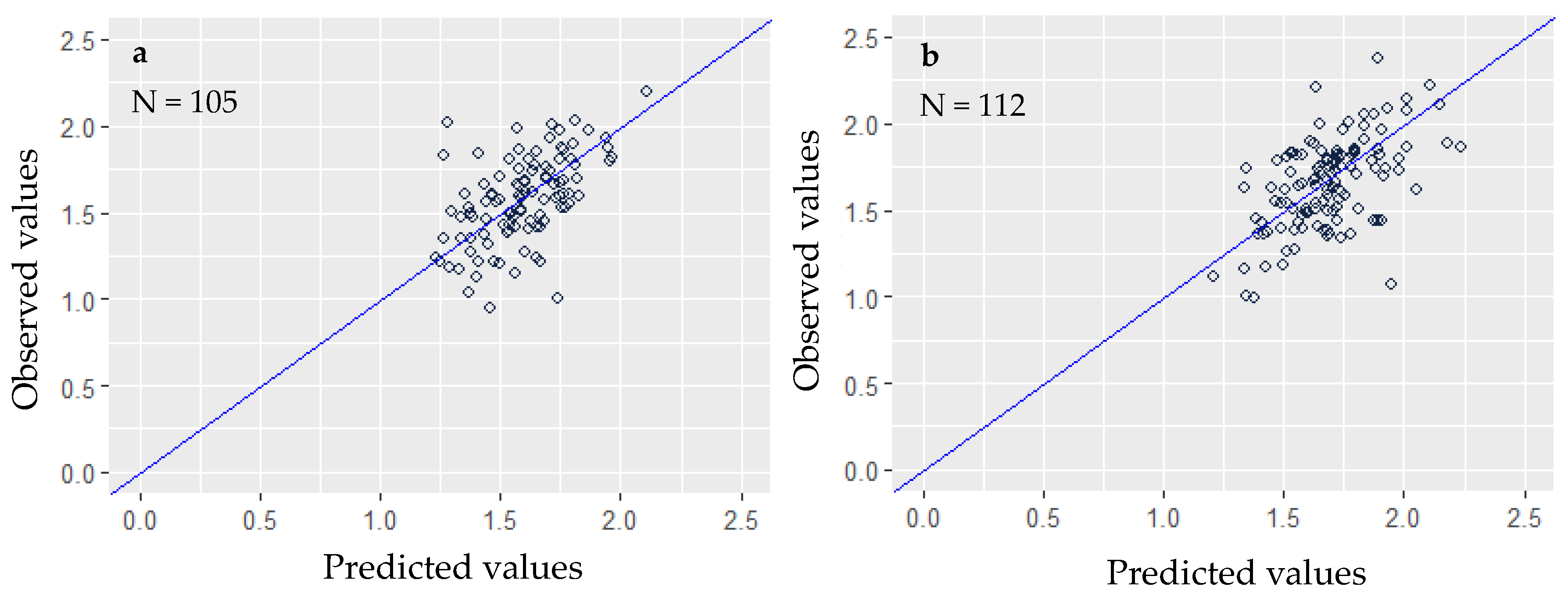
3.3. Estimating Merchantable Top Length
Bias in white spruce prediction of total tree height (MEP) was 0.0245 m and the average size of the prediction error was 0.3987 m (MAEP) (Figure 8a). The value of MSEP was 0.2805 and the prediction coefficient of determination was 0.5084. Bias in balsam fir prediction of total tree height (MEP) was 0.1748 m and the average size of the prediction error was 0.4452 m (MAEP) (Figure 8b). The value of MSEP was 0.3838 and the prediction coefficient of determination was 0.5788.
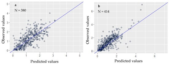
Figure 8.
Observed merchantable top length plotted against predicted values with a line of unity for (a) white spruce and (b) balsam fir.
3.4. Spatialization Tool
Outputs of the spatialization tool varied according to the StanForD version. In StanForD, the only output was a shapefile displaying a summary of NUWM per harvest area (Figure 9a). In StanForD 2010, two shapefiles were provided (1) the location of the harvested stems along with its volume of NUWM and (2) the sum of NUWM volume per hectare (100 × 100 m grid) (Figure 9b).
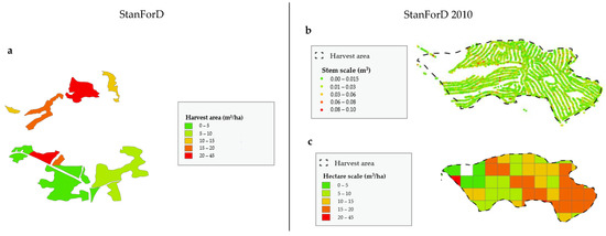
Figure 9.
Graphical display of the outputs obtained from the NUWM spatialization tool; for StanForD (a) at a harvest area scale and StandForD 2010 (b) at a stem scale, (c) at a hectare scale (100 × 100 m grid).
3.5. Explorative Comparison
The explorative comparison highlighted key information that could be useful for decision making (Table 5). As indicated in the methodology, a literature review and our expert knowledge were used to orient the explorative comparison.
Table 5.
Summary of exploratory comparison of technical aspect.
The estimation of the cost for the conventional field method and the OBC method was calculated as follows. For the conventional field method, 25 transects at a cost of 115 $/transect are required to assess the amount of NUWM remaining after harvesting for a harvest area of 60 ha (average size of harvest areas in the region). Therefore, these mandatory field inventories are averaging costs of 50 $/hectare. Single-grip harvesters are normally operating double shifts of 10-h per day, thus totaling 85 h per week. Within this time and based on the silvicultural treatments applied in the region, they commonly harvest 1 ha per 10-h shift for a total of 8.5 ha per week. A technician requires approx. 1 h (at a cost of 75–80 $/h) to download the production and positioning data for one week, therefore, providing an average cost of 8.8–9.4 $/ha for the OBC method. It is likely that the OBC method developed cannot exclusively replace the conventional field inventory and that a complimentary field inventory might be warranted in problematic areas. For this reason, we decided to add a 40% buffer to the costs of the OBC method, which represents approximately 3.5–3.8 $/ha and brings the estimated total costs to 12.3–13.2 $/ha.
Snow was often a limiting factor in the realization of NWUM inventories. Consequently, conventional field method can only be made during the summer. Conversely, OBC method is not weather dependent, thereby making the results available on a per day basis. Seasonal workers need to be hired in the summer for the conventional field method, as on the contrary, the OBC method does not require new hiring.
As the conventional field method is executed by forests technicians, there is always a potential for human error and the precision of the measurement is of 2 cm classes. As for the OBC method, the predominant error possible is harvester imprecision and the precision of the measurement is at a millimetric precision. Between the two methods, the scale is different, as plot scale is used for the conventional method and tree scale is used for the OBC method.
4. Discussion
4.1. Study Limitations
The algorithms and spatialization tool were developed only for white spruce and balsam fir found within the Gaspésie region of Canada. Therefore, a direct transfer of these developments to other species or jurisdictions is not recommended without performing further calibration. Furthermore, results obtained in this project are somewhat sensitive to the experience of harvester operators and product specifications.
4.2. Estimation of Merchantable Top Section
Results suggest that by combining Varjo’s model with the linear regression for individual stems, it is possible to reconstruct and estimate the section of NUWM using OBC data. It was first necessary to estimate the top length (Ltop) to improve the response of the merchantable top length at diameter 9.1 cm over bark. Varjo’s predictive equations have proven to be useful in reconstructing individual trees from harvester data [12,14,26,27]. Originally, Varjo’s predictive equations were developed for stems with a small-end diameter of the top log (SEDUBTL) between 5 and 10 cm and with a minimum log length of 1.5 m [14,20,27]. Equation (1) for predicting Ltop was based on Varjo’s (1995) model but with SEDUBTL replaced by SEDOBTL as a predictor. The value of SEDOBTL for white spruce ranged from 7.30–18.10 cm, and the minimum log length was 2.76 m amongst the 355 trees used in estimating the parameters of Equation (1). The value of SEDOBTL for balsam fir ranged from 7.80–23.50 cm, and the minimum log length was 2.76 m amongst the 390 trees used in estimating the parameters of Equation (1). The minimum log length of 1.5 m is respected in this study considering that the smallest product assortment is of 2.5 m. The range of SEDOBTL in our study was similar to the results reported by Lu et al. for their model developed for radiata pine [14]. However, our SEDOBTL remained more variable than the diameters used in Varjo’s model that was developed for spruce, birch, and pine in Finland.
For both species, when the predicted Ltop was added to total log length and stump height (Equation (2)), the total tree height had a smaller bias than the predicted Ltop (white spruce: 0.4064 to 0.8603; balsam fir: 0.5249 to 0.7312.) The same phenomenon was described by Lu et al. (2021), showing similar range of differences [14]. Prediction values of white spruce total length above stump level was generally underestimated by the model (MEP: −0.0069 m). Despite not being originally developed for balsam fir, Varjo’s model could indeed be used to estimate Ltop and total length above stump. Bias in balsam fir prediction of total tree length above stump (MEP) was 0.0958 m and suggested an overestimation compared to observed values.
Similarly, Lu et al. [7] used Varjo’s model to estimate total height of radiata pine trees in plantation stands and their results were more uniform than the ones reported in our study. The lower variation can be explained by differing stand characteristics, as our study was in natural forests, which creates a more natural variability than what is commonly encountered in plantations. A difference between total field length and OBC total length of stems was observed. In large part, this difference is linked to the creation of wood discs that are missing from OBC data but measured in the field. Wood discs are common occurrences when an operator performs a so-called “free-cut” to reset the length measurement of the OBC. Close monitoring of the operators work method is recommended. It can create an underestimation of predicted total length above stump level (Figure 7).
Varjo’s model was selected for its both its applicability and simplicity and the fact that it was already used for spruce in Finland. Another model, proposed by Shan [15], was developed to reconstruct stem height of radiata pines and generally showed better results and less variability than Varjo’s model. Estimations of parameters for Shan’s model and a comparison between both models with more data could lead to interesting information to improve our total length estimation.
To our knowledge, this study represents the first rigorous attempt at developing a model for predicting merchantable length of the top section in order to estimate quantities of NUWM from CTL harvester data. The estimation of Ltopm (DOBM = 9.1 cm) was obtained with linear regression and parameters estimated for each individual trees. The main explanation of differences between observed and predicted length values is a divergence of small-end diameter of the top log in the OBC data and the observed large-end diameter of the top. This can be explained by the presence of forks or large diameter branches, whereby a considerable fluctuation in diameter within a short distance is observed. As the small-end diameter of the last log increases, length prediction becomes less accurate and may need more analysis in the future. However, these instances did not occur frequently in our dataset. If length prediction is the variable of interest, other models may be applied to obtain a clearer result.
4.3. Spatialization Tool
Stem spatialization tools using OBC data already exist and are used in other countries. For instance, Woo et al. (2021) [24] developed a software named Forest Inventory Electronic Live Data (FIELD) to analyze StanForD .pri files and implement a real-time geospatial harvesting residue monitoring system. Biomass availability after harvesting was estimated using suitable allometric equations. In our case, merchantable volume is evaluated instead of biomass. Moreover, the spatialization tool we developed uses both StanForD and StanForD 2010, as both standards are frequently used in eastern Canada. With StanForD, the output is not spatializing the NUWM volume by stem since none of the harvesters used the manufacturer GPS and the .pri files does not contain tree-level timestamp information. For this reason, StanForD does not provide the same precision as StanForD 2010, which spatializes NUWM volume by stem. If high precision is needed, the change from StanForD to StanForD 2010 to position stems or the purchase of manufacturer GPS to have position of the stem in .pri files should be considered. Moreover, to spatialize the NUWM volume into a harvest area, a simple deduction is made using the start and end time of the project in the OBC with timestamp of GPS tracklog. Errors can be created in the positioning if both OBC and GPS times are not synced. It is also important to mention that when using a .hpr file, the software tool spatializes the location of the harvester at the time a stem is harvested and processed, and not the exact location of the stem since the GPS is normally located in the cabin and not on the boom. Therefore, the exact location of the stem might differ by several meters.
4.4. Explorative Comparison
Industrial stakeholders in the Gaspésie region will be able to estimate the volumes of NUWM for white spruce and balsam fir using a tool integrated into the OBC in real-time and visualize the spatial distribution of NUWM within the harvest site. The explorative comparison highlighted a possible reduction approx. 36.8 $/ha when using OBC data instead of the conventional NUWM field inventory. We are not implying that the OBC method developed can exclusively replace the conventional field inventory, but it can be used to identify problematic areas, which could in turn become target areas for complimentary field inventories. Moreover, the delays associated with conventional field inventory of NUWM will therefore be reduced and the information will be accessible more quickly and easily, thus facilitating decision related to forest operations and industrial planning. Considering that the aim of the inventory is to avoid unnecessary waste of wood on public lands, the evaluation of NUWM, through the developed algorithms, can be performed year-long and could allow industrial stakeholders to correct nonconformities when the agreement is not respected. At the moment, corrections are difficult to make since NUWM field inventories are only done in summer and the delay between data acquisition and processing can take up to one year.
5. Conclusions
The aim of this research was to estimate the volume of NUWM after mechanized CTL harvesting operations using data from the OBC. Mathematic algorithms were developed with data from five study areas located in Gaspésie region of Canada. Results obtained in this study demonstrated the effectiveness of using StanForD files to estimate the length of the top section on a per tree basis for white spruce and balsam fir. A spatialization tool was developed to position NUWM volume. Industrial stakeholders of the region will be able to estimate the volume of NUWM for white spruce and balsam fir using the developed tool in real-time and visualize the spatial distribution of NUWM within the harvest site. Finally, the explorative comparison highlighted the cost-saving opportunity (approx. 36.8 $/ha) linked with using OBD data to estimate NUWM, while allowing a more rapid response time to address any corrections by targeting problematic areas.
Although the case study was site specific, the problem associated with the lack of pulpwood takers is not unique to the region. With certain regional adaptations, the algorithms and tool developed could be used in other regions of Canada to support the competitiveness of the forest sector. Further studies should focus on developing the mathematic algorithms for others commercial species and to develop an integrated software that collects and analyses data automatically.
Author Contributions
Conceptualization, M.D. and E.R.L.; methodology, M.D. and E.R.L.; software, Alexandre Morneau, M.D., E.R.L.; data collection, M.D.; data analysis, M.D. and E.R.L.; writing, M.D. and E.R.L.; supervision, E.R.L.; funding acquisition, E.R.L. All authors have read and agreed to the published version of the manuscript.
Funding
This master’s thesis was funded by MITACS (grant number IT18990) and the APC was covered by the Université Laval.
Institutional Review Board Statement
Not applicable.
Informed Consent Statement
Not applicable.
Data Availability Statement
Not applicable.
Acknowledgments
We would like to thank industrial and governmental stakeholders in Gaspésie for their support and information provided during every step of the study. We would also like to thank every worker on the project for their hard work in the field and during the development of the spatialization tool. Lastly, we wish to acknowledge the constructive comments received by the reviewers.
Conflicts of Interest
The authors declare no conflict of interest.
References
- Labelle, E.R.; Jaeger, D.; Poltorak, B.J. Assessing the Ability of Hardwood and Softwood Brush Mats to Distribute Applied Loads. Croat. J. For. Eng. 2015, 36, 227–242. [Google Scholar]
- Uusitalo, J. Introduction to Forest Operations and Technology, 2010th ed.; JVP Forest Systems Oy: Tampere, Finland, 2010; ISBN 952-92-5269-2. [Google Scholar]
- Labelle, E.R.; Jaeger, D. Soil Compaction Caused by Cut-to-Length Forest Operations and Possible Short-Term Natural Rehabilitation of Soil Density. Soil Sci. Soc. Am. J. 2011, 75, 2314–2329. [Google Scholar] [CrossRef] [Green Version]
- Éditeur officiel du Québec. Loi sur L’aménagement Durable du Territoire Forestier; Gouvernement du Québec: Quebec, QC, Canada, 2021; Chapter A-18.1; p. 88.
- Plasse, J.-G. Inventaire de la Matière Ligneuse Utilisable mais non Récoltée dans les Aires de Coupe: Instructions; Ministère des Ressources Naturelles, Division des Permis D’intervention et de L’utilisation Polyvalente, Direction de L’assistance Technique: Charlesbourg, QC, Canada, 2000.
- Proulx, G.; Beaudoin, J.-M.; Asselin, H.; Bouthillier, L.; Théberge, D. Untapped Potential? Attitudes and Behaviours of Forestry Employers toward the Indigenous Workforce in Quebec, Canada. Can. J. For. Res. 2020, 50, 413–421. [Google Scholar] [CrossRef]
- Kemmerer, J.; Labelle, E.R. Using Harvester Data from On-Board Computers: A Review of Key Findings, Opportunities and Challenges. Eur. J. For. Res. 2021, 140, 1–17. [Google Scholar] [CrossRef]
- Roth, G. StanForD as a Data Source for Forest Management: A Forest Stand Reconciliation Implementation Case Study; University of Canterbury: Christchurch, New Zealand, 2016. [Google Scholar]
- Latvia University of Life Sciences and Technologies; Strubergs, A.; Lazdins, A.; Latvia State Forest Research Institute ‘Silava’; Sisenis, L. Latvia University of Life Sciences and Technologies Evaluation of Compliance of Existing Forest Machine Information Systems for the Implementation of the Standard StanForD 2010; Research for Rural Development. International Scientific Conference Proceedings (Latvia): Jelgava, Latvia, 2020; pp. 66–72. [Google Scholar]
- Terblanche, M. Unlocking the Potential of Harvester On-Board-Computer Data in the South African Forestry Value Chain; Stellenbosch University: Stellenbosch, South Africa, 2019. [Google Scholar]
- Ghaffariyan, M.R. Evaluating the Machine Utilisation Rate of Harvester and Forwarder Using On-Board Computers in Southern Tasmania (Australia). J. For. Sci. 2016, 61, 277–281. [Google Scholar] [CrossRef]
- Vesa, L.; Palander, T. Modeling Stump Biomass of Stands Using Harvester Measurements for Adaptive Energy Wood Procurement Systems. Energy 2010, 35, 3717–3721. [Google Scholar] [CrossRef]
- Rodrigues, C.K.; Lopes, E.S.; Figueiredo Filho, A.; Pelissari, A.L.; Silva, M.K.C. Modeling Residual Biomass from Mechanized Wood Harvesting with Data Measured by Forest Harvester. An. Acad. Bras. Ciênc. 2019, 91, e20190194. [Google Scholar] [CrossRef] [PubMed]
- Lu, K.; Bi, H.; Watt, D.; Strandgard, M.; Li, Y. Reconstructing the Size of Individual Trees Using Log Data from Cut-to-Length Harvesters in Pinus Radiata Plantations: A Case Study in NSW, Australia. J. For. Res. 2018, 29, 13–33. [Google Scholar] [CrossRef] [Green Version]
- Shan, C.; Bi, H.; Watt, D.; Li, Y.; Strandgard, M.; Ghaffariyan, M.R. A New Model for Predicting the Total Tree Height for Stems Cut-to-Length by Harvesters in Pinus Radiata Plantations. J. For. Res. 2021, 32, 21–41. [Google Scholar] [CrossRef] [Green Version]
- Ministère des Forêts, de la Faune et des Parcs Ressources et industries forestières du Québec, portrait statistique 2020. 2020. p. 160. Available online: https://mffp.gouv.qc.ca/wp-content/uploads/PortraitStatistique_2020.pdf (accessed on 12 May 2022).
- Labelle, E.; Huss, L. Creation of Value through a Harvester On-Board Bucking Optimization System Operated in a Spruce Stand. Silva Fenn. 2018, 52, 9947. [Google Scholar] [CrossRef]
- Team, R.C. R: A Language and Environment for Statistical Computing; R Foundation for Statistical Computing: Vienna, Austria, 2018. [Google Scholar]
- Perron, J.-Y.; Québec (Province) Direction des Inventaires Forestiers. Tarif de Cubage Général: Volume Marchand Brut; Direction des Inventaires Forestiers: Quebec, QC, Canada, 2003; ISBN 978-2-551-21866-0.
- Varjo, J. Puutavaran Mittauksen Kehittämistutkimuksia 1989–1993; Metsäntutkimuslaitoksen Tiedonantoja; Metsäntutkimuslaitos: Helsinki, Finland, 1995; ISBN 978-951-40-1434-5. [Google Scholar]
- Craigmile, P.F. EnvStats: An R Package for Environmental Statistics by Steven P. Millard. J. Agric. Biol. Environ. Stat. 2017, 22, 107–109. [Google Scholar] [CrossRef]
- Snowdon, P. A Ratio Estimator for Bias Correction in Logarithmic Regressions. Can. J. For. Res. 1991, 21, 720–724. [Google Scholar] [CrossRef]
- Huang, S.; Yang, Y.; Wang, Y. A Critical Look at Procedures for Validating Growth and Yield Models. In Modelling Forest Systems, Proceedings of the Workshop on the Interface between Reality, Modelling and the Parameter Estimation Processes, Sesimbra, Portugal, 2–5 June 2002; Amaro, A., Reed, D., Soares, P., Eds.; CABI: Wallingford, UK, 2003; pp. 271–292. ISBN 978-0-85199-693-6. [Google Scholar]
- Woo, H.; Acuna, M.; Choi, B.; Han, S. FIELD: A Software Tool That Integrates Harvester Data and Allometric Equations for a Dynamic Estimation of Forest Harvesting Residues. Forests 2021, 12, 834. [Google Scholar] [CrossRef]
- Ministère des Forêts, de la Faune et des Parcs Devis technique: Inventaires de suivi de la matière ligneuse non utilisée (MLNU)—Méthode du transect 2018. Available online: https://mffp.gouv.qc.ca/publications/forets/entreprises/Norme_echange_numerique_BGA_2018_19.pdf (accessed on 12 May 2022).
- Palander, T.; Vesa, L.; Tokola, T.; Pihlaja, P.; Ovaskainen, H. Modelling the Stump Biomass of Stands for Energy Production Using a Harvester Data Management System. Biosyst. Eng. 2009, 102, 69–74. [Google Scholar] [CrossRef]
- Siipilehto, J.; Lindeman, H.; Vastaranta, M.; Yu, X.; Uusitalo, J. Reliability of the Predicted Stand Structure for Clear-Cut Stands Using Optional Methods: Airborne Laser Scanning-Based Methods, Smartphone-Based Forest Inventory Application Trestima and Pre-Harvest Measurement Tool EMO. Silva Fenn. 2016, 50, 1568. [Google Scholar] [CrossRef] [Green Version]


Publisher’s Note: MDPI stays neutral with regard to jurisdictional claims in published maps and institutional affiliations. |
© 2022 by the authors. Licensee MDPI, Basel, Switzerland. This article is an open access article distributed under the terms and conditions of the Creative Commons Attribution (CC BY) license (https://creativecommons.org/licenses/by/4.0/).