
Global Sensitivity Analysis of the LPJ Model for Larix olgensis Henry Forests NPP in Jilin Province, China


Abstract
:1. Introduction
2. Material and Methods
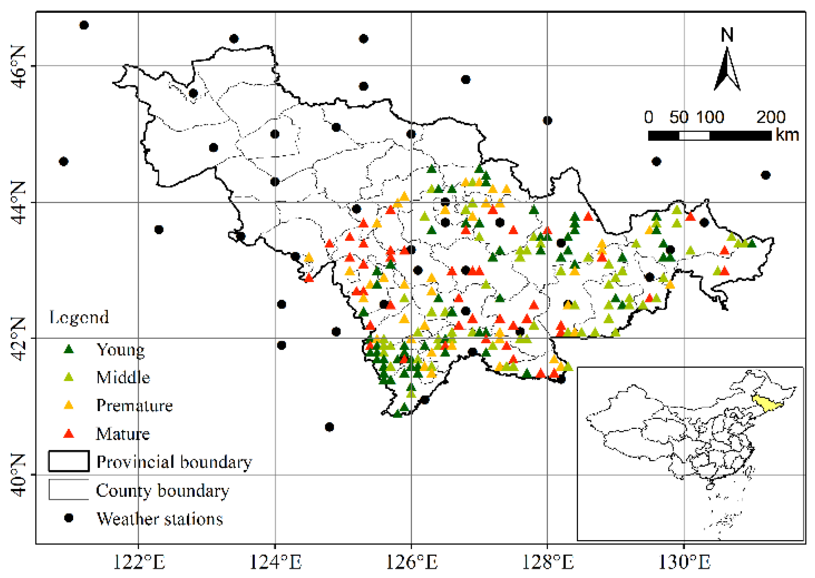
2.1. Site Description
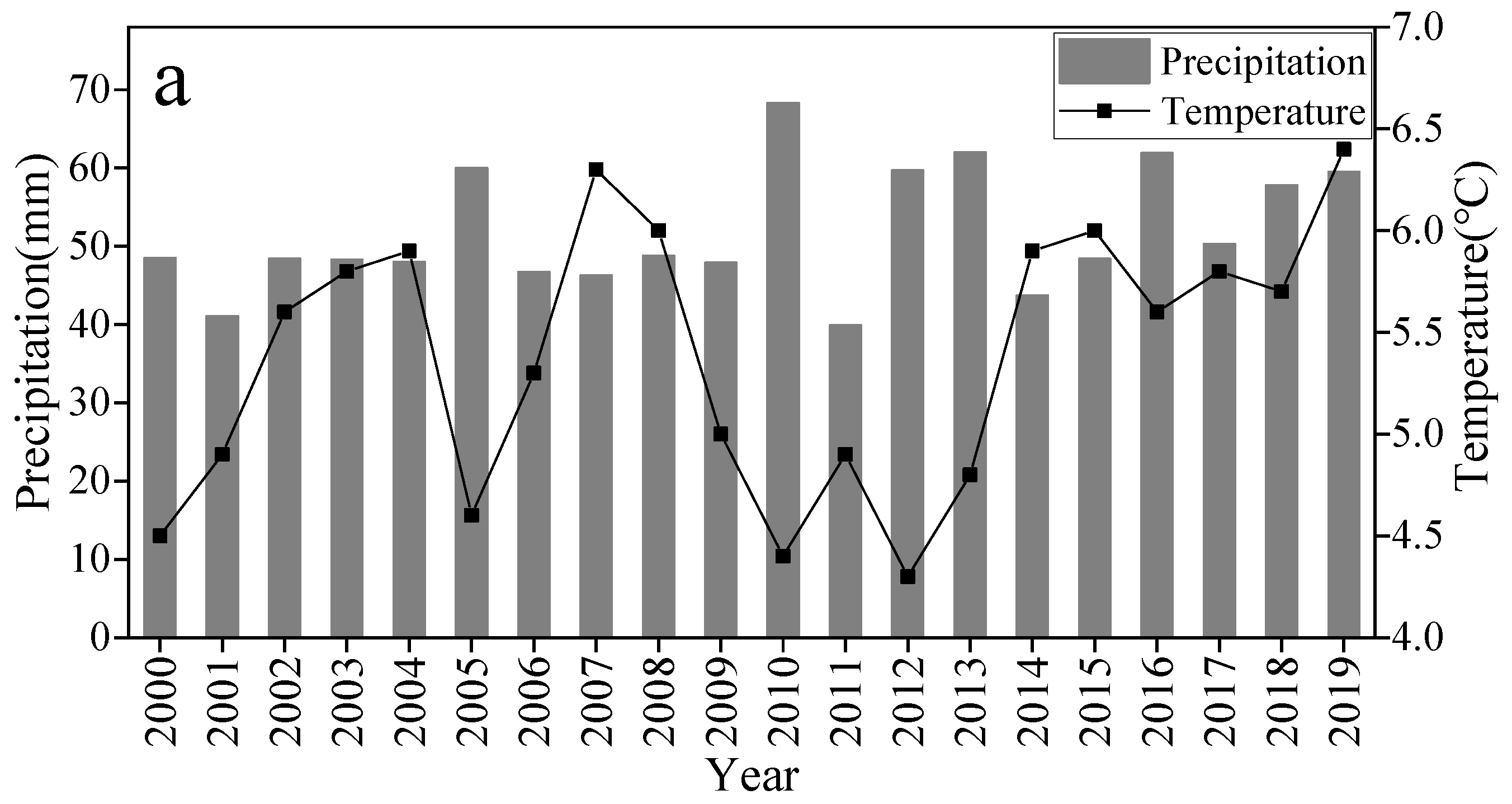
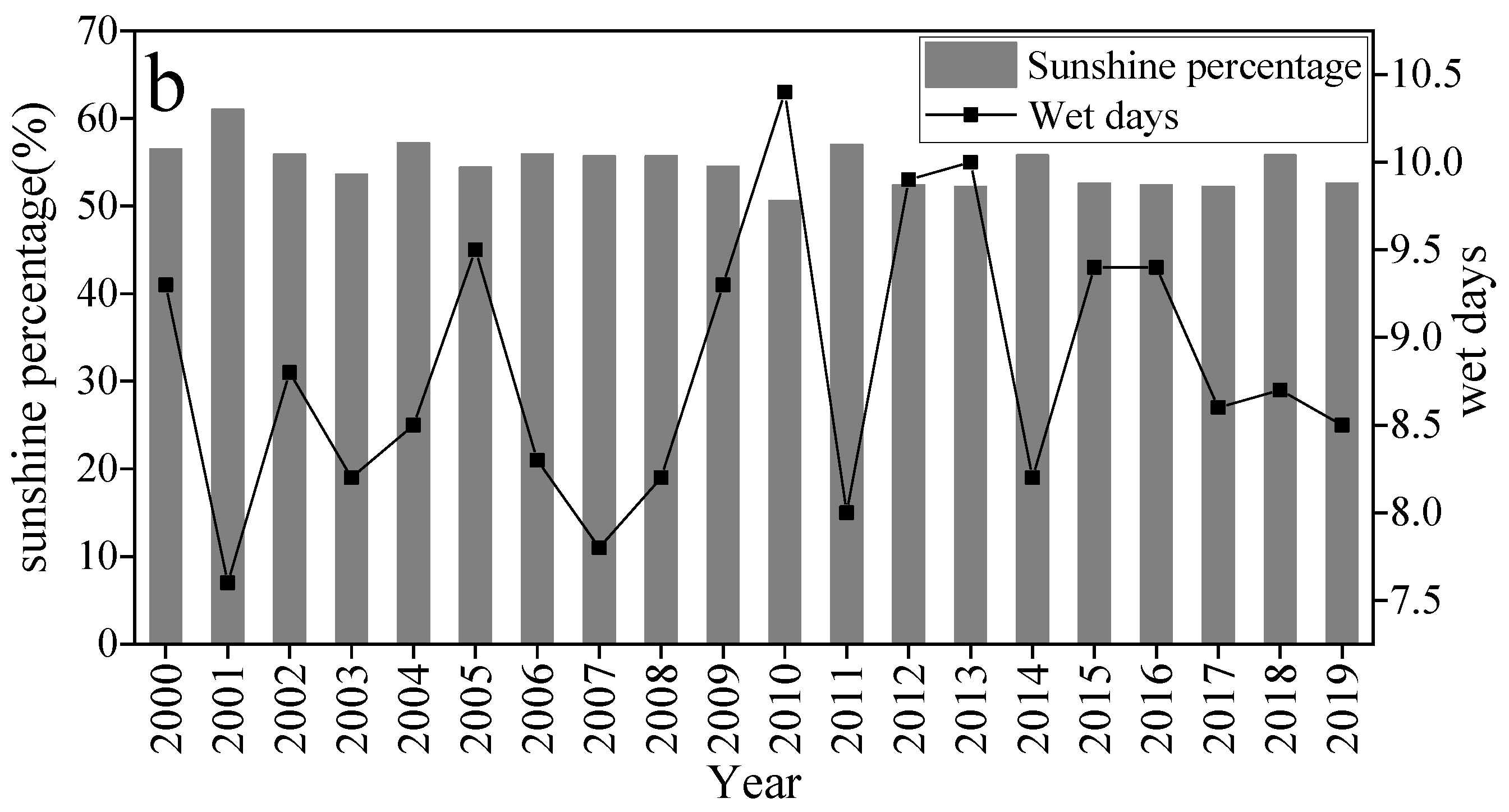
2.2. Climate Data
2.3. Description of the LPJ Model and Input Parameter Setting
2.3.1. Description of LPJ-DGVM
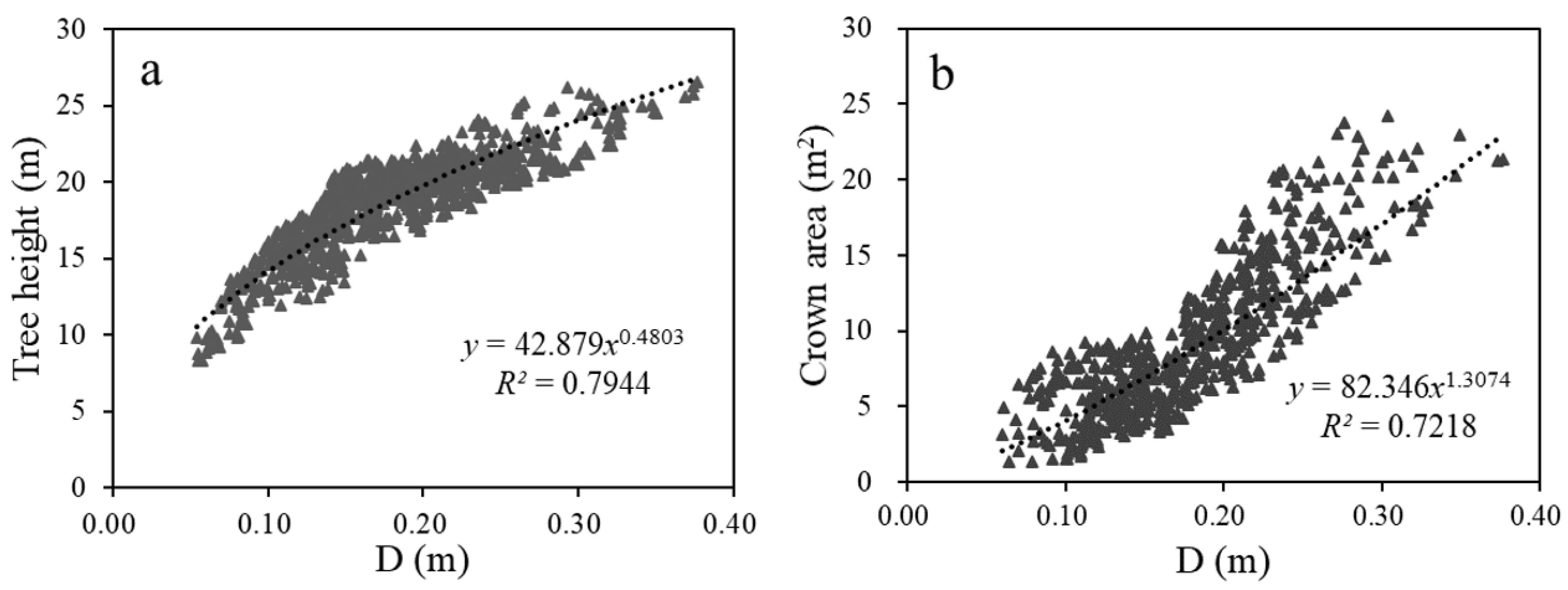
2.3.2. Input Parameters Setting
2.4. Sensitivity Analysis Methods and Scheme
2.4.1. EFAST Method
2.4.2. Morris Method
2.4.3. Sensitivity Analysis Scheme
2.5. Remote Sensing Observation Data of NPP
2.6. Measured Data and Accuracy Evaluation Index
3. Results
3.1. LPJ Model Output NPP Based on the EFAST and Morris Methods
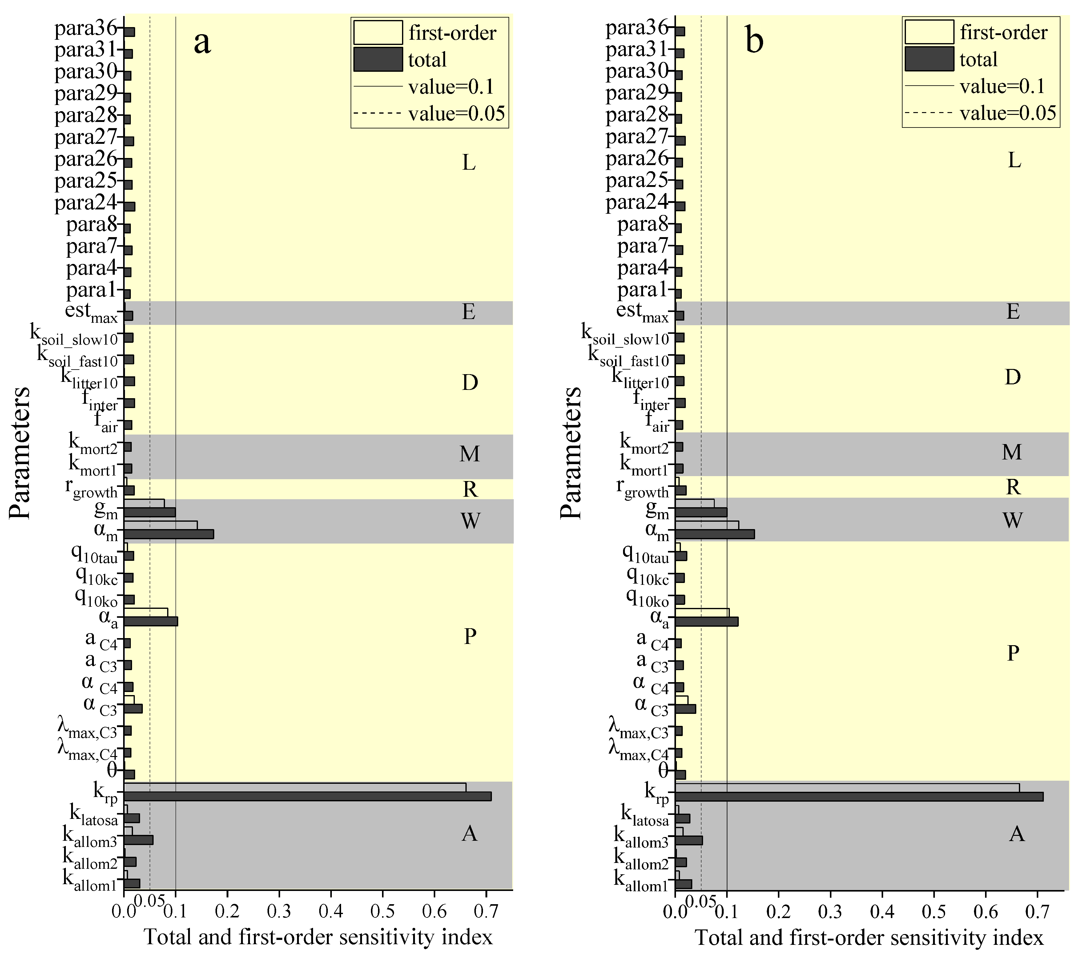
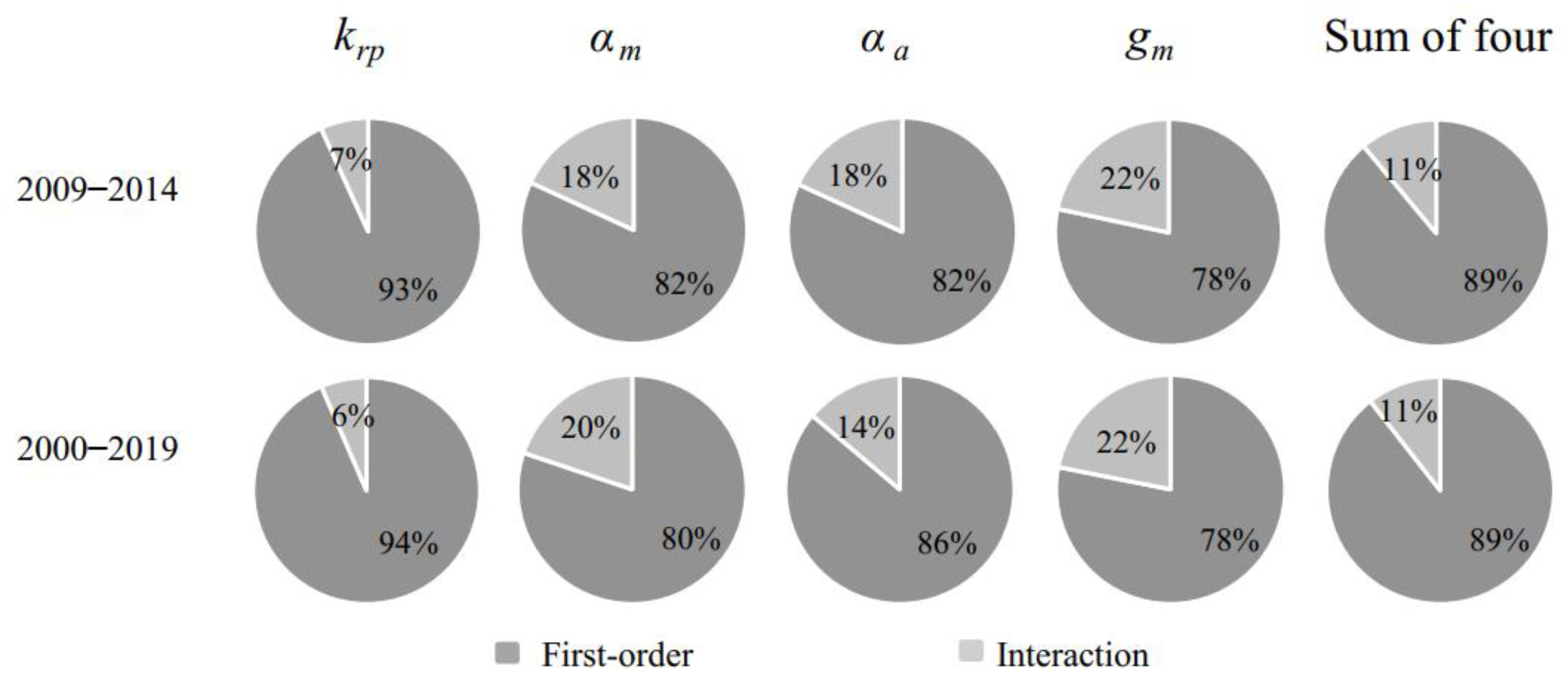
3.2. Importance Ranking of the LPJ Model to NPP Sensitivity Based on the EFAST Method
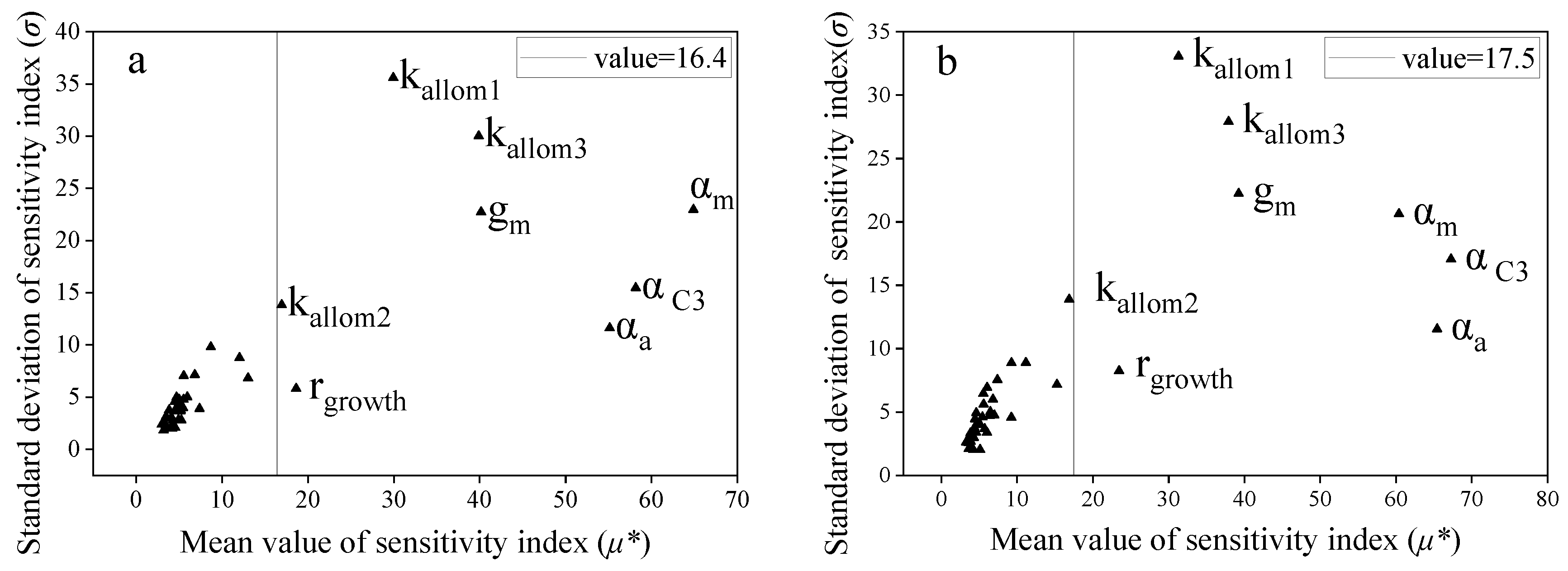
3.3. Importance Ranking of the LPJ Model to NPP Sensitivity Based on the Morris Method
3.4. Comparison of Analysis Results Based on the EFAST and Morris Methods
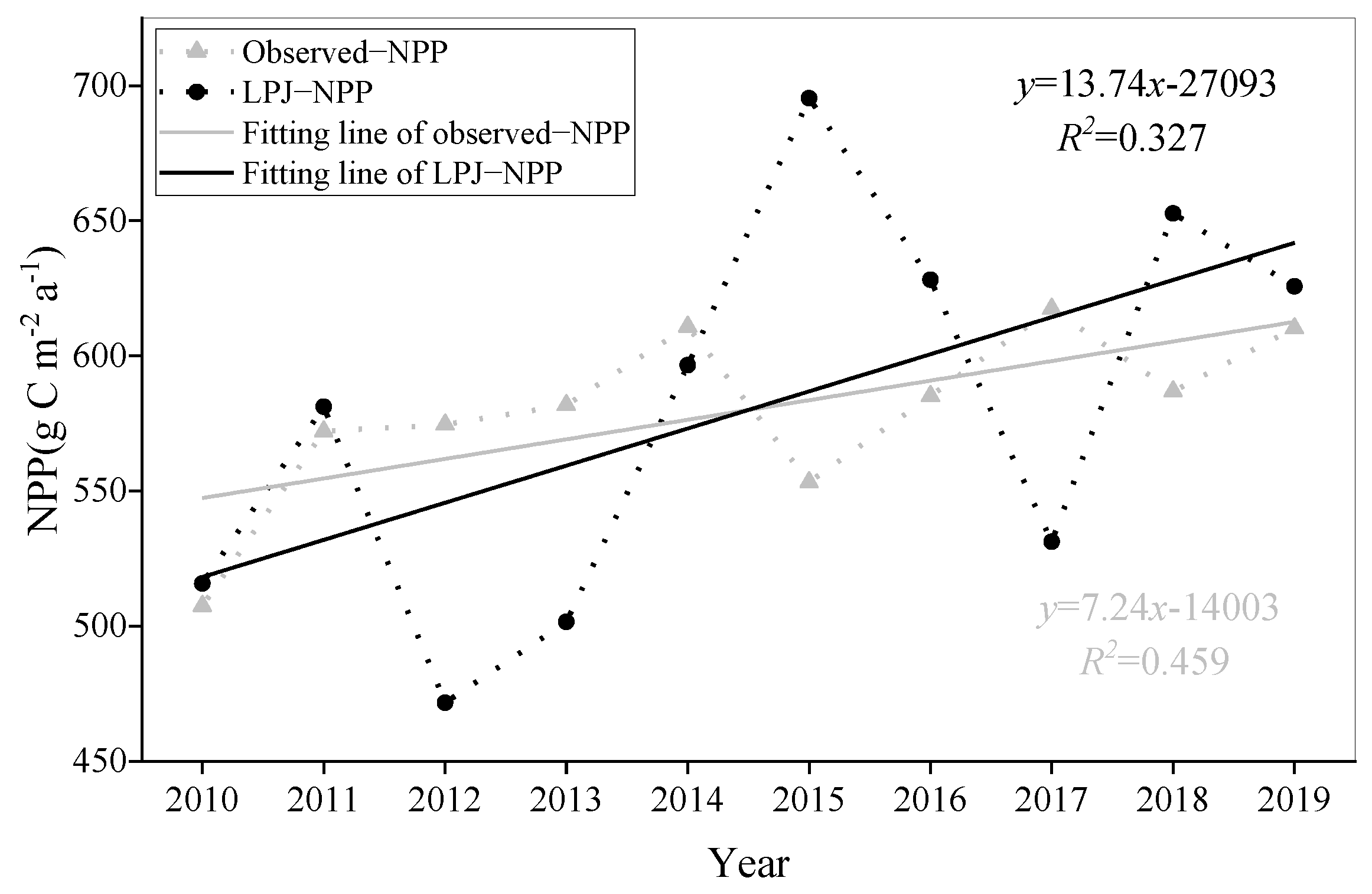
3.5. Model Optimization and Accuracy Verification
4. Discussion
4.1. Comparison between the EFAST and Morris Method
4.2. Uncertainty of Sensitivity Analysis Method
4.3. Uncertainty of the LPJ Model
5. Conclusions
Author Contributions
Funding
Institutional Review Board Statement
Informed Consent Statement
Data Availability Statement
Acknowledgments
Conflicts of Interest
References
- Sallaba, F.; Lehsten, D.; Seaquist, J.; Sykes, M.T. A rapid NPP meta-model for current and future climate and CO2 scenarios in Europe. Ecol. Model. 2015, 302, 29–41. [Google Scholar] [CrossRef]
- Kong, R.; Zhang, Z.; Zhang, F.; Tian, J.; Zhu, B.; Zhu, M.; Wang, Y. Spatial and temporal dynamics of forest carbon storage and its driving factors in the Yangtze River Basin. Res. Soil Water Conserv. 2020, 27, 60–66. [Google Scholar]
- Dubey, S.; Sharma, A.; Panchariya, V.K.; Goyal, M.K.; Surampalli, R.Y.; Zhang, T.C. Regional sustainable development of renewable natural resources using Net Primary Productivity on a global scale. Ecol. Indic. 2021, 127, 107768. [Google Scholar] [CrossRef]
- Yan, Y.; Wu, C.; Wen, Y. Determining the impacts of climate change and urban expansion on net primary productivity using the spatio-temporal fusion of remote sensing data. Ecol. Indic. 2021, 127, 107737. [Google Scholar] [CrossRef]
- Xie, Y.; Wang, H.; Lei, X. Effects of climate change on net primary productivity in Larix olgensis plantations based on process modeling. Chin. J. Plant Ecol. 2017, 41, 826–839. [Google Scholar]
- Li, Y.; Wang, Y.; Sun, Y.; Lei, Y.; Shao, W.; Li, J. Temporal-spatial characteristics of NPP and its response to climate change of Larix forests in Jilin Province. Acta Ecol. Sin. 2022, 42, 947–959. [Google Scholar]
- Jiang, Y.; Zhuang, Q.; Sitch, S.; O’Donnell, J.A.; Kicklighter, D.; Sokolov, A.; Melillo, J. Importance of soil thermal regime in terrestrial ecosystem carbon dynamics in the circumpolar north. Glob. Planet Chang. 2016, 142, 28–40. [Google Scholar] [CrossRef] [Green Version]
- Cui, B.; Zheng, J.; Tuerxun, H.; Duan, S.; Du, M. Spatio-temporal characteristics of grassland net primary productivity(NPP) in the Tarim River basin. Acta Prataculturae Sin. 2020, 29, 1–13. [Google Scholar]
- Smith, B.; Prentice, I.C.; Syks, M.T. Representation of vegetation dynamics in the modelling of terrestrial ecosystems: Comparing two contrasting approaches within European climate space. Glob. Energy Biogeogr. 2001, 10, 621–637. [Google Scholar] [CrossRef]
- Sitch, S.; Smith, B.; Prentice, I.C.; Arneth, A.; Bondeau, A.; Cramer, W.; Kaplan, J.O.; Levis, S.; Lucht, W.; Sykes, M.T.; et al. Evaluation of ecosystem dynamics, plant geography and terrestrial carbon cycling in the LP dynamic global vegetation model. Glob. Chang. Biol. 2003, 9, 161–185. [Google Scholar] [CrossRef]
- Sakschewski, B.; von Bloh, W.; Boit, A.; Rammig, A.; Kattge, J.; Poorter, L.; Peñuelas, J.; Thonicke, K. Leaf and stem economics spectra drive diversity of functional plant traits in a dynamic global vegetation model. Glob. Chang. Biol. 2015, 21, 2711–2725. [Google Scholar] [CrossRef] [PubMed]
- Renwick, K.M.; Fellows, A.; Flerchinger, G.N.; Lohse, K.A.; Clark, P.E.; Smith, W.K.; Emmett, K.; Poulter, B. Modeling phenological controls on carbon dynamics in dryland sagebrush ecosystems. Agric. For. Meteorol. 2019, 274, 85–94. [Google Scholar] [CrossRef]
- Morris, M.D. Factorial Sampling Plans for Preliminary Computational Experiments. Technometrics 1991, 33, 161–174. [Google Scholar] [CrossRef]
- Saltelli, A.; Tarantola, S.; Chan, K.P.S. A Quantitative Model-Independent Method for Global Sensitivity Analysis of Model Output. Technometrics 1999, 41, 39–56. [Google Scholar] [CrossRef]
- DeJonge, K.C.; Ascough, J.C.; Ahmadi, M.; Andales, A.A.; Arabi, M. Global sensitivity and uncertainty analysis of a dynamic agroecosystem model under different irrigation treatments. Ecol. Model. 2012, 231, 113–125. [Google Scholar] [CrossRef]
- Cui, J.; Shao, G.; Lin, J.; Ding, M. Global Sensitivity Analysis of CROPGRO-Tomato Model Parameters Based on EFAST Method. Trans. Chin. Soc. Agric. Mach. 2020, 51, 237–244. [Google Scholar]
- Zhang, T.; Sun, R.; Hu, B.; Feng, L. Using simulated annealing algorithm to optimize the parameters of Biome-BGC model. Chin. J. Ecol. 2011, 30, 408–414. [Google Scholar]
- Crosetto, M.; Tarantola, S.; Saltelli, A. Sensitivity and uncertainty analysis in spatial modelling based on GIS. Agric. Ecosyst. Environ. 2000, 81, 71–79. [Google Scholar] [CrossRef]
- Jiang, Z.; Chen, Z.; Zhou, Q.; Ren, J. Global sensitivity analysis of CERES-Wheat model parameters. Trans. CSAE 2011, 27, 236–242. [Google Scholar]
- Klepper, O. Multivariate aspects of model uncertainty analysis: Tools for sensitivity analysis and calibration. Ecol. Model. 1997, 101, 1–13. [Google Scholar] [CrossRef]
- Confalonieri, R.; Bellocchi, G.; Tarantola, S.; Acutis, M.; Donatelli, M.; Genovese, G. Sensitivity analysis of the rice model WARM in Europe: Exploring the effects of different locations, climates and methods of analysis on model sensitivity to crop parameters. Environ. Modell. Softw. 2010, 25, 479–488. [Google Scholar] [CrossRef]
- Xing, H.; Xiang, S.; Xu, X.; Chen, Y.; Feng, H.; Yang, G.; Chen, Z. Global Sensitivity Analysis of AquaCrop Crop Model Parameters Based on EFAST Method. Sci. Agric. Sin. 2017, 50, 64–76. [Google Scholar]
- Saltelli, A.; Annoni, P. How to avoid a perfunctory sensitivity analysis. Environ. Modell. Softw. 2010, 25, 1508–1517. [Google Scholar] [CrossRef]
- Zhang, N.; Zhang, Q.; Yu, H.; Cheng, M.; Dong, S. Sensitivity analysis for parameters of crop growth simulation model. J. Zhejiang Univ. Agric. Life Sci. 2018, 44, 107–115. [Google Scholar]
- Sobol, I.M. Global sensitivity indices for nonlinear mathematical models and their Monte Carlo estimates. Math. Comput. Simulat. 2001, 55, 271–280. [Google Scholar] [CrossRef]
- Li, B.; Li, C.; Yao, M.; Wei, X.; Bao, Z.; Sun, X. Sensitivity and Uncertainty Analysis for CROPGRO-Tomato Model at Different Irrigation Levels. J. Shenyang Agric. Univ. 2020, 51, 153–161. [Google Scholar]
- Pappas, C.; Fatichi, S.; Leuzinger, S.; Wolf, A.; Burlando, P. Sensitivity analysis of a process-based ecosystem model: Pinpointing parameterization and structural issues. J. Geophys. Res. Biogeosci. 2013, 118, 505–528. [Google Scholar] [CrossRef]
- Vazquez-Cruz, M.A.; Guzman-Cruz, R.; Lopez-Cruz, I.L.; Cornejo-Perez, O.; Torres-Pacheco, I.; Guevara-Gonzalez, R.G. Global sensitivity analysis by means of EFAST and Sobol methods and calibration of reduced state-variable TOMGRO model using genetic algorithms. Comput. Electron. Agric. 2014, 100, 1–12. [Google Scholar] [CrossRef]
- Jin, X.; Li, Z.; Nie, C.; Xu, X.; Feng, H.; Guo, W.; Wang, J. Parameter sensitivity analysis of the AquaCrop model based on extended fourier amplitude sensitivity under different agro-meteorological conditions and application. Field Crops Res. 2018, 226, 1–15. [Google Scholar] [CrossRef]
- Xing, A.; Zhuo, Z.; Zhao, Y.; Li, Y.; Huang, Y. Sensitivity Analysis of WOFOST Model Crop Parameters under Different Production Levels Based on EFAST Method. Trans. Chin. Soc. Agric. Mach. 2020, 51, 161–171. [Google Scholar]
- Editorial Committee of Vegetation Map of China. Vegetation map of the People’s Republic of China; Geological Publishing House: Beijing, China, 2007. [Google Scholar]
- Shinozaki, K.; Yoda, K.; Hozumi, K.; Kira, T. A quantitative analysis of plant form-the pipe model theory I. basic analyses. Jpn. J. Ecol. 1964, 14, 97–105. [Google Scholar]
- Shinozaki, K.; Yoda, K.; Hozumi, K.; Kira, T. A quantitative analysis of plant form-the pipe model theory II. further evidence of the theory and its application in forest ecology. Jpn. J. Ecol. 1964, 14, 133–139. [Google Scholar]
- Waring, R.H.; Schroeder, P.E.; Oren, R. Application of the pipe model theory to predict canopy leaf area. Can. J. For. Res. 1982, 12, 556–560. [Google Scholar] [CrossRef]
- Magnani, F.; Leonardi, S.; Tognetti, R.; Grace, J.; Borghetti, M. Modelling the surface conductance of a broad-leaf canopy: Effects of partial decoupling from the atmosphere. Plant Cell Environ. 1998, 21, 867–879. [Google Scholar] [CrossRef]
- Monteith, J.L. Accommodation between transpiring vegetation and the convective boundary layer. J. Hydrol. 1995, 166, 251–263. [Google Scholar] [CrossRef]
- Zaehle, S.; Sitch, S.; Smith, B.; Hatterman, F. Effects of parameter uncertainties on the modeling of terrestrial biosphere dynamics. Glob. Biogeochem. Cycles 2005, 19, 1–16. [Google Scholar] [CrossRef]
- Prentice, I.C.; Sykes, M.T.; Cramer, W. A simulation model for the transient effects of climate change on forest landscapes. Ecol. Model. 1993, 65, 51–70. [Google Scholar] [CrossRef]
- Huang, S.; Titus, S.J.; Wiens, D.P. Comparison of nonlinear height-diameter functions for major Alberta tree species. Can. J. For. Res. 1992, 22, 1297–1304. [Google Scholar] [CrossRef]
- Enquist, B.J. Global Allocation Rules for Patterns of Biomass Partitioning in Seed Plants. Science 2002, 295, 1517–1520. [Google Scholar] [CrossRef] [Green Version]
- Collatz, G.J.; Berry, J.A.; Farquhar, G.D.; Pierce, J. The relationship between the Rubisco reaction mechanism and models of photosynthesis. Plant Cell Environ. 1990, 13, 219–225. [Google Scholar] [CrossRef]
- Haxeltine, A.; Pretience, I.C. BIOME: An equilibrium terrestrial biosphere model based on ecophysiological constrains, resource availability, and competition among plant functional types. Funct. Ecol. 1996, 10, 551–561. [Google Scholar] [CrossRef]
- Farquhar, G.D.; von Caemmerer, S.; Berry, J.A. A biochemical model of photosynthetic CO2 assimilation in leaves of C3 species. Planta 1980, 149, 78–90. [Google Scholar] [CrossRef] [Green Version]
- Haxeltine, A.; Prentice, I.C.L.U.; Creswell, I.D. A coupled carbon and water flux model to predict vegetation structure. J. Veg. Sci. 1996, 7, 651–666. [Google Scholar] [CrossRef]
- Sprugel, D.G.; Ryan, M.G.; Renée, J.; Brooks, K.A.V.A. Respiration from the Organ Level to the Stand Level to the Stand. Resour. Physiol. Conifers 1995, 8, 255–299. [Google Scholar]
- Jenkinson, D.S. The Turnover of Organic Carbon and Nitrogen in Soil. Philos. Trans. R. Soc. Lond. B 1990, 329, 361–368. [Google Scholar]
- Foley, J.A. An equilibrium model of the terrestrial carbon budget. Tellus 1995, 47B, 310–319. [Google Scholar] [CrossRef] [Green Version]
- Wu, L.; Zhang, F.; Fan, J.; Zhou, H.; Xing, Y.; Qiang, S. Sensitivity and uncertainty analysis for CROPGRO-cotton model at different irrigation levels. Trans. Chin. Soc. Agric. Eng. 2015, 31, 55–64. [Google Scholar]
- Campolongo, F.; Cariboni, J.; Saltelli, A. An effective screening design for sensitivity analysis of large models. Environ. Modell. Softw. 2007, 22, 1509–1518. [Google Scholar] [CrossRef]
- Dong, L.; Zhang, L.; Li, F. Developing additive systems of biomass equations for nine hardwood species in Northeast China. Trees 2015, 29, 1149–1163. [Google Scholar] [CrossRef]
- Wang, C. Biomass allometric equations for 10 co-occurring tree species in Chinese temperate forests. For. Ecol. Manag. 2006, 222, 9–16. [Google Scholar] [CrossRef]
- Fang, J.; Liu, G.; Xu, S. Biomass and net production of forest vegetation in China. Acta Ecol. Sin. 1996, 16, 497–508. [Google Scholar]
- Ma, R. Dynamic Simulation and Analysis of Carbon and Water Fluxes in China Based on Model-Data Fusion; University of Chinese Academy of Sciences: Beijing, China, 2018. [Google Scholar]
- Song, M.; Feng, H.; Li, Z.; Gao, J. Global Sensitivity Analyses of DSSAT-CERES-Wheat Model Using Morris and EFAST Methods. Trans. Chin. Soc. Agric. Mach. 2014, 45, 124–166. [Google Scholar]
- Shin, M.; Guillaume, J.H.A.; Croke, B.F.W.; Jakeman, A.J. Addressing ten questions about conceptual rainfall–runoff models with global sensitivity analyses in R. J. Hydrol. 2013, 503, 135–152. [Google Scholar] [CrossRef]
- Vanuytrecht, E.; Raes, D.; Willems, P. Global sensitivity analysis of yield output from the water productivity model. Environ. Modell. Softw. 2014, 51, 323–332. [Google Scholar] [CrossRef] [Green Version]
- He, L. Response of Net Primary Productivity of Larix.x olgensis Forest to Climate Change in Northeast China. Master’s Thesis, Beijing Forestry University, Beijing, China, 2015. [Google Scholar]
- Zhao, D.; Wu, S.; Yin, Y. Variation trends of natural vegetation net primary productivity in China under climate change scenario. Chin. J. Appl. Ecol. 2011, 22, 897–904. [Google Scholar]
- Wang, X.; Sun, Y.; Ma, W. Biomass and carbon storage distribution of different density in Larix olgensis plantation. J. Fujian Coll. For. 2011, 31, 221–226. [Google Scholar]


| No | Parameter | Default Value | Lower Value | Upper Value | Description | Reference |
|---|---|---|---|---|---|---|
| 1 | kallom1-A | 100 | 90 | 110 | parameter in Equation (4) | [37] |
| 2 | kallom2-A | 40 | 36 | 44 | parameter in Equation (3) | [39] |
| 3 | kallom3-A | 0.50 | 0.45 | 0.55 | parameter in Equation (3) | [39] |
| 4 | klatosa-A | 4000 | 3600 | 4400 | parameter (cross-sectional area) in Equation (1) | [34] |
| 5 | krp-A | 1.60 | 1.44 | 1.76 | parameter in allometric Equation (4) | [40] |
| 6 | θ-P | 0.70 | 0.63 | 0.77 | colimitation (shape) parameter | [41] |
| 7 | λmax,C4-P | 0.40 | 0.36 | 0.44 | optimal ratio of intercellular to ambient CO2 concentration in C4 plants | [41] |
| 8 | λmax,C3-P | 0.80 | 0.72 | 0.88 | optimal ratio of intercellular to ambient CO2 concentration in C3 plants | [42] |
| 9 | α C3-P | 0.080 | 0.072 | 0.088 | intrinsic quantum efficiency of CO2 uptake in C3 plants | [43] |
| 10 | α C4-P | 0.0530 | 0.0477 | 0.0583 | intrinsic quantum efficiency of CO2 uptake in C4 plants | [41] |
| 11 | a C3-P | 0.0150 | 0.0135 | 0.0165 | leaf respiration as a fraction of Robisco capacity for C3 plants | [43] |
| 12 | a C4-P | 0.020 | 0.018 | 0.022 | leaf respiration as a fraction of vmax for C4 plants | [41] |
| 13 | αa-P | 0.450 | 0.405 | 0.495 | fraction of PAR assimilated at ecosystem level relative to leaf level | [44] |
| 14 | q10ko-P | 1.20 | 1.08 | 1.32 | q10 for temperature-sensitive parameter ko | [42] |
| 15 | q10kc-P | 2.10 | 1.89 | 2.31 | q10 for temperature-sensitive parameter kc | [42] |
| 16 | q10tau-P | 0.570 | 0.513 | 0.627 | q10 for temperature-sensitive parameter tau | [42] |
| 17 | αm-W | 1.40 | 1.26 | 1.54 | Priestley-Taylor coefficient (Demand) | [36] |
| 18 | gm-W | 3.26 | 2.934 | 3.586 | empirical parameter in demand function | [35] |
| 19 | rgrowth-R | 0.25 | 0.225 | 0.275 | Proportion of growth respiration per unit NPP | [45] |
| 20 | kmort1-M | 0.050 | 0.045 | 0.055 | asymptotic maximum mortality rate (/year) | [37] |
| 21 | kmort2-M | 0.50 | 0.45 | 0.55 | mortality equation | [37] |
| 22 | fair-D | 0.70 | 0.63 | 0.77 | fraction of litter decomposition going directly into the atmosphere | [46] |
| 23 | finter-D | 0.980 | 0.882 | 1.078 | fraction of litter entering fast soil decomposition pool | [47] |
| 24 | klitter10-D | 0.350 | 0.315 | 0.385 | litter decomposition rate at 10 deg C (/year) | [47] |
| 25 | ksoil_fast10-D | 0.030 | 0.027 | 0.033 | fast pool decomposition rate at 10 deg C (/year) | [47] |
| 26 | ksoil_slow10-D | 0.0010 | 0.0009 | 0.0011 | slow pool decomposition rate at 10 deg C (/year) | [47] |
| 27 | estmax-E | 0.120 | 0.108 | 0.132 | maximum sapling establishment rate | [37] |
| 28 | para1-L | 0.70 | 0.63 | 0.77 | fraction of roots in upper soil layer | [10] |
| 29 | para4-L | 0.30 | 0.27 | 0.33 | canopy conductance component (gmin, mm/s) not associated with photosynthesis | [42] |
| 30 | para7-L | 100 | 90 | 110 | maximum foliar N content (mg/g) | [42] |
| 31 | para8-L | 0.120 | 0.108 | 0.132 | fire resistance index | [10] |
| 32 | para24-L | −4.0 | −3.6 | −4.4 | low temperature limit for CO2 uptake CO2 | [10] |
| 33 | para25-L | 15.0 | 13.5 | 16.5 | lower range of temperature optimum for photosynthesis | [10] |
| 34 | para26-L | 30.0 | 27.0 | 33.0 | upper range of temperature optimum for photosynthesis | [10] |
| 35 | para27-L | 42.0 | 37.8 | 46.2 | high temperature limit for CO2 uptake | [10] |
| 36 | para28-L | −13.0 | −11.7 | −14.3 | minimum coldest monthly mean temperature | [10] |
| 37 | para29-L | 3.0 | 2.7 | 3.3 | maximum coldest monthly mean temperature | [10] |
| 38 | para30-L | 900 | 810 | 990 | minimum growing degree days (at above 5 °C) | [10] |
| 39 | para31-L | 1000 | 900 | 1100 | upper limit of temperature of the warmest month | [10] |
| 40 | para36-L | 0.060 | 0.054 | 0.066 | interception storage parameter, unitless | [10] |
| NO | Parameters | 2009–2014 | 2000–2019 | ||
|---|---|---|---|---|---|
| EFAST Rank | Morris Rank | EFAST Rank | Morris Rank | ||
| 1 | kallom1-A | 7 | 7 | 7 | 7 |
| 2 | kallom2-A | 9 | 9 | 10 | 9 |
| 3 | kallom3-A | 5 | 6 | 5 | 6 |
| 4 | klatosa-A | 8 | 12 | 8 | 12 |
| 5 | krp-A | 1 | 1 | 1 | 1 |
| 6 | θ-P | 12 | 23 | 12 | 13 |
| 7 | λmax,C4-P | 35 | 31 | 34 | 37 |
| 8 | λmax,C3-P | 32 | 25 | 33 | 26 |
| 9 | α C3-P | 6 | 3 | 6 | 2 |
| 10 | α C4-P | 22 | 36 | 24 | 40 |
| 11 | a C3-P | 30 | 13 | 25 | 15 |
| 12 | a C4-P | 37 | 20 | 38 | 27 |
| 13 | αa-P | 3 | 4 | 3 | 3 |
| 14 | αm-W | 2 | 2 | 2 | 4 |
| 15 | gm-W | 4 | 5 | 4 | 5 |
| 16 | kmort1-M | 29 | 14 | 26 | 14 |
| 17 | kmort2-M | 31 | 37 | 30 | 38 |
| 18 | fair-D | 27 | 21 | 29 | 17 |
| 19 | finter-D | 13 | 15 | 13 | 16 |
| 20 | estmax-E | 23 | 11 | 23 | 11 |
| 21 | rgrowth-R | 15 | 8 | 11 | 8 |
| 22 | q10ko-P | 16 | 32 | 17 | 32 |
| 23 | q10kc-P | 20 | 24 | 18 | 20 |
| 24 | q10tau-P | 17 | 10 | 9 | 10 |
| 25 | klitter10-D | 11 | 38 | 22 | 36 |
| 26 | ksoil_fast10-D | 19 | 33 | 19 | 31 |
| 27 | ksoil_slow10-D | 21 | 39 | 20 | 35 |
| 28 | para1-L | 40 | 17 | 40 | 28 |
| 29 | para4-L | 33 | 40 | 35 | 34 |
| 30 | para7-L | 26 | 19 | 28 | 29 |
| 31 | para8-L | 39 | 22 | 39 | 23 |
| 32 | para24-L | 10 | 28 | 15 | 24 |
| 33 | para25-L | 25 | 18 | 27 | 18 |
| 34 | para26-L | 28 | 35 | 31 | 39 |
| 35 | para27-L | 18 | 27 | 14 | 33 |
| 36 | para28-L | 38 | 16 | 37 | 19 |
| 37 | para29-L | 36 | 26 | 36 | 22 |
| 38 | para30-L | 34 | 34 | 32 | 30 |
| 39 | para31-L | 24 | 30 | 21 | 21 |
| 40 | para36-L | 14 | 29 | 16 | 25 |
| Parameters of Analysis | 2009–2014 | 2000–2019 |
|---|---|---|
| All parameters | 0.501 ** | 0.674 ** |
| Both sensitively | 0.883 ** | 0.738 * |
| Periods | Methods | Before Optimization | After Optimization | ||
|---|---|---|---|---|---|
| MRE (%) | MAE (g C m−2 a−1) | MRE (%) | MAE (g C m−2 a−1) | ||
| 2009–2014 | LPJ–Measured | 50.8 | 193.2 | 40.2 | 153.0 |
| 2010–2019 | LPJ–MODIS NPP | 11.4 | 65.5 | 9.8 | 56.7 |
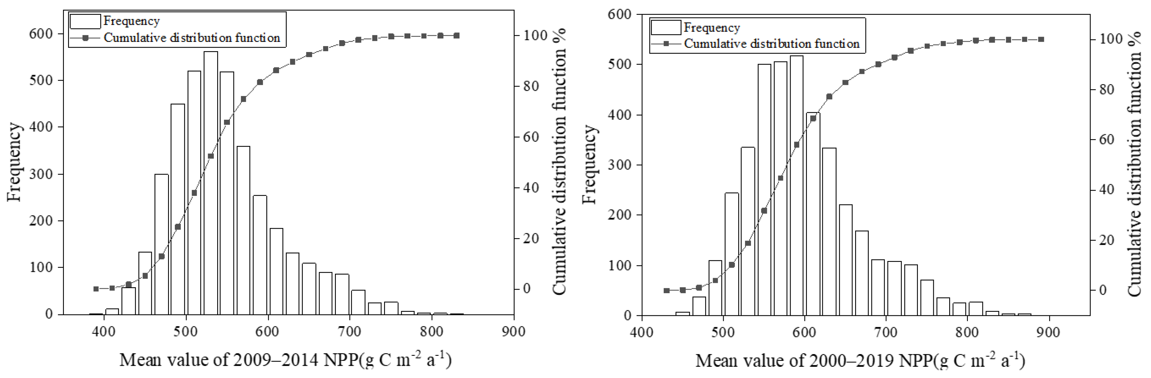
| Period of NPP | The MODIS NPP | Medium Value | 95% Confidence Interval Lower Limit | 95% Confidence Interval Upper Limit | Standard Deviation |
|---|---|---|---|---|---|
| 2009–2014 | 573 | 536 | 418 | 675 | 66 |
| 2000–2019 | 580 | 587 | 463 | 734 | 69 |
Publisher’s Note: MDPI stays neutral with regard to jurisdictional claims in published maps and institutional affiliations. |
© 2022 by the authors. Licensee MDPI, Basel, Switzerland. This article is an open access article distributed under the terms and conditions of the Creative Commons Attribution (CC BY) license (https://creativecommons.org/licenses/by/4.0/).
Share and Cite
Li, Y.; Wang, Y.; Sun, Y.; Li, J. Global Sensitivity Analysis of the LPJ Model for Larix olgensis Henry Forests NPP in Jilin Province, China. Forests 2022, 13, 874. https://doi.org/10.3390/f13060874
Li Y, Wang Y, Sun Y, Li J. Global Sensitivity Analysis of the LPJ Model for Larix olgensis Henry Forests NPP in Jilin Province, China. Forests. 2022; 13(6):874. https://doi.org/10.3390/f13060874
Chicago/Turabian StyleLi, Yun, Yifu Wang, Yujun Sun, and Jie Li. 2022. "Global Sensitivity Analysis of the LPJ Model for Larix olgensis Henry Forests NPP in Jilin Province, China" Forests 13, no. 6: 874. https://doi.org/10.3390/f13060874
APA StyleLi, Y., Wang, Y., Sun, Y., & Li, J. (2022). Global Sensitivity Analysis of the LPJ Model for Larix olgensis Henry Forests NPP in Jilin Province, China. Forests, 13(6), 874. https://doi.org/10.3390/f13060874