Article

Causes of Changing Woodland Landscape Patterns in Southern China

1
School of Geography and Environmental Engineering, Gannan Normal University, Ganzhou 341000, China
2
Department of Surveying and Geo-Informatics, Jiangxi College of Applied Technology, Ganzhou 341000, China
3
Ganzhou Bureau of Natural Resources, Ganzhou 341000, China
*
Author to whom correspondence should be addressed.
Forests 2022, 13(12), 2183; https://doi.org/10.3390/f13122183
Submission received: 16 October 2022 / Revised: 10 December 2022 / Accepted: 16 December 2022 / Published: 19 December 2022

Abstract

:
Forests are composed of landscape spatial units (patches) of different sizes, shapes, and characteristics. The forest landscape pattern and its trends are closely related to resistance to disturbance, restoration, stability, and the biodiversity of the forest landscape and directly influence the benefits and sustainable exploitation of forest landscape resources. Therefore, forest landscape patterns and the driving forces have increasingly attracted the attention of researchers. The present study analyzed the spatial and temporal dynamics of woodland landscape patterns in typical hilly mountainous areas in southern China using ArcGIS, landscape pattern index, and morphological spatial pattern analysis. Meanwhile, a logistic regression model was used to analyze the drivers of woodland change in Anyuan County from three aspects: natural, geographic location, and socio-economic conditions. The total area of woodland decreased during the 10-year study period, with a net decrease of 4959.27 ha, mainly due to conversion into cultivated land, garden land, and construction land. Patch density, edge density, and aggregation index of woodlands increased over time, indicating enhanced fragmentation, stable and complex patch edges, and increased patch connectivity. Conversely, the highest patch index values exhibited decreasing trends, indicating decreases in the dominant patch type. Morphological spatial pattern analysis results showed that the core area was dominant and the islet area increased over time, which also indicates enhanced fragmentation. Forest landscape change is the result of environmental change, ecological processes, and human disturbance, with geographical location and social economy having greater influences on forest landscape change. Human activities such as navel orange cultivation, returning cultivated land to forest, and land occupation for construction were the major factors driving woodland change. The results provide reference that could facilitate forest management and sustainable forest resource utilization.

1. Introduction

Forests play fundamental roles in the maintenance of terrestrial ecosystems, safeguarding of basic human living conditions, and mitigation of climate change; in addition, they are essential for sustainable socio-economic development [1,2]. As the carrier of forest resources, forest land is not only the basis for sustainable forestry development but also a prerequisite for the maintenance of the ecological services of forests [3,4,5]. Different forest landscape systems are observed under various forest ecological types, and geographical, climatic, and socio-economic conditions, leading to distinct and diverse forest landscape mosaics [6,7,8].
The study of forest landscape structure, function, the dynamics and mechanisms of mutual influence and control, and the rational spatial configuration according to the characteristics of different ecosystems helps to reveal the relationship between the natural environment and human society. It can also facilitate the maximization the production potential of natural resources [9,10,11,12]. Consequently, forest landscape patterns have increasingly attracted the attention of various stakeholders, particularly changes in forest landscape patterns and the driving forces over the long term [13].
Current studies on forest landscape patterns have focused on heterogeneity over time and space. For example, Wu et al. quantified the degree of human interference by constructing the Hemeroby index (HI) and explored the spatio-temporal characteristics of landscape patterns and human interference in the course of urbanization [14]. Coops et al. combined remote sensing techniques with landscape pattern indices to analyze changes in forest fragmentation following beetle infestation over time [15]. However, landscape pattern research mainly analyzes the type, quantity, and spatial distribution and configuration of landscape units, which are largely limited to two-dimensional planes [16]. In contrast, the introduction of morphological spatial pattern analysis (MSPA) into forest landscape analysis can facilitate the rapid and intuitive identification of spatial morphology [17], which is conducive for the optimization of the ecological security barrier system, establishment of ecological corridors and biodiversity conservation networks, forest ecological network construction, and decision-making and data support in forest resource management [18,19,20]. Therefore, the application of MSPA to landscape ecology is increasing.
The forest landscape pattern refers to the composition and spatial distribution of forest in the landscape, reflecting landscape heterogeneity, and is the result of interactions between natural and human factors across space and time [21]. It is of great scientific significance to clarify the characteristics and driving forces of spatial and temporal changes in forest landscape, which can facilitate the understanding of shifts in regional ecological environment, rational use of resources, and harmonization of the relationship between people and land [22]. Therefore, researchers have applied different variables to explain the forces that drive woodland change; however, previous analyses often ignore the driving influence of socio-economic factors or the spatial heterogeneity of institutions (policies) on land use change, making it difficult to objectively and accurately reveal the causes of woodland change [23]. As for the research methodology, the influence of each driving factor in different geographical locations is mainly obtained through Moran’s I index analysis [24], geographically weighted regression and principal component analysis [25]; however, at present, there are fewer studies that involve exploring the influence of each factor on the degree of land use from the overall to the local level [26]. Logistic regression models can not only take account of the spatial heterogeneity of land use change drivers but can also quantify the relationship between regional land use dynamics and drivers, such as social, economic, technological, policy, and natural environment factors [24]. In recent years, some scholars have used logistic regression models to analyze the drivers of urban spatial expansion, arable land change, and land use change; however, they are relatively less frequently applied to woodland landscape analysis [25].
The Gannan area of Jiangxi Province is an ecological geographical barrier in southern China. The forest ecosystem in the area is influenced by geographical and human factors simultaneously so that a single landscape index may not adequately reflect changes in forest landscape [27]. Consequently, there is an urgent need for a variety of methods to analyze forest landscape trends. Therefore, the present study attempts to collect landscape pattern data and morphological data and systematically analyze the spatio-temporal changes in forest landscapes in Anyuan County, a typical county in the hilly mountains of southern Jiangxi Province, using the logistic regression model to analyze the factors driving forest landscape change in the region. The objectives of the present study are: (1) to determine the change of woodland area using a land-use conversion matrix; (2) to explore the change of woodland landscape using morphological spatial pattern analysis (MSPA) and landscape pattern indices; (3) to identify the drivers of forest landscape change using a logistic model; and (4) to propose an optimal management strategy for the forest landscape in the study area.

2. Materials and Methods

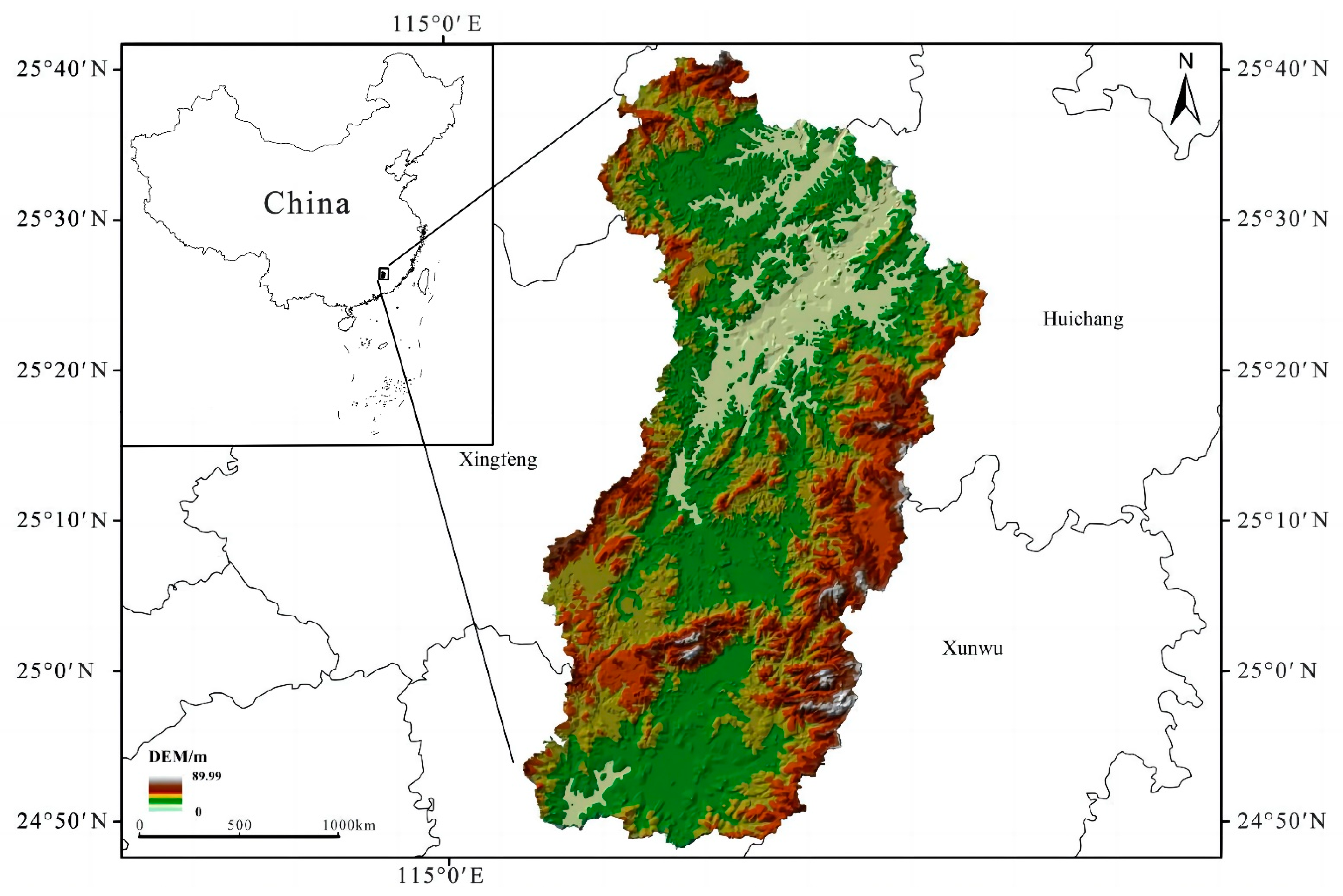
2.1. Study Area and Data Collection

Anyuan County is located in the south of Jiangxi Province, China (115°9′112″–115°37′13″ E, 24°52′18″–25°36′52″ N). It belongs to the humid monsoon hanging area at the southern edge of the Central Subtropics. The topography of the study area is undulating and mainly consists of low and medium mountains and hills extending from the Nanling Mountain Range (Figure 1). The total land area of Anyuan County is 235,924.1 ha, out of which 83.4% is mountainous. Anyuan County is a typical inland mountainous area dominated by woodlands and is the origin of the upper Ganjiang River (Yangtze River system) and the Dongjiang River (Pearl River system), which provide drinking water for Hong Kong.

2.2. Data Sources and Processing

The 2009 Second National Land Survey Data, 2014 Land Use Change Data and 2019 National Land Survey Data were obtained from the Natural Resources Bureau of Anyuan County. Digital elevation model (DEM) data for Anyuan County with a 30 m × 30 m resolution were downloaded from the Geospatial Data Cloud (http://www.gscloud.cn, 17 August 2022) to extract slope and topographic relief information. Soil texture and soil type maps of Anyuan County were also extracted from the corresponding maps of Jiangxi Province. Socio-economic statistical data, such as navel orange cultivation, returning farmland to forest, and land occupancy for construction were derived from the Anyuan County Statistical Yearbook (Table 1). Using ArcGIS v10.6 (ESRI Inc., Redlands, CA, USA), land use data for 2009, 2014, and 2019 were used to reclassify the study area into seven categories: farmland, garden land, woodland, grassland, construction land, water area, and other land. Woodland was further divided into forestland, shrubland, and other woodland (Figure 2).

2.3. Transfer Matrix-Based Analysis of Woodland Change

The land use transfer matrix was derived from a Markov model to analyze woodland change in the study area [28,29]. The Markov model can not only quantify the transferred area between different land use types but also reveal the rate of land use transfer. The equation is as follows:
D i j = i j n [ S i j S i ] × 100 %
where Dij is the proportion of land use type i converted to type j in the study period; Si is the initial area of land use type i in the study area; Si−j is the area of land use type i converted to type j in a study period; and n is the number of land use types converted in the study area. Vector data were converted into 30 m × 30 m raster data and subjected to overlay analysis using ArcGIS v10.6. The results were imported into Excel v2021 (Microsoft Corp., Redmond, WA, USA), and a pivot table was inserted to derive the woodlands transfer matrix.

2.4. Selection of Landscape Pattern Indices

Landscape pattern analysis is the core process in landscape ecology research. Understanding the relationships between landscape elements and the development of landscape patterns is essential for accurately revealing trends in ecological environment change. At present, this analysis is the most widely used method to quantitatively study the landscape pattern [30,31,32]. Therefore, 11 landscape pattern indices were selected based on their ecological connotations combined with the characteristics of landscape types in the study area. Five indices were selected at the level of patch type: largest patch index (LPI), aggregation index (AI), landscape shape index (LSI), patch density (PD), and edge density (ED). Six indices were selected at the landscape level: patch density (PD), number of patches (NP), edge density (ED), landscape shape index (LSI), aggregation index (AI), and Shannon diversity (SHDI). The ecological connotations of each index are summarized in Table 2 [33,34,35]. The landscape indices of woodlands in each study period were calculated using Fragstats v4.2 (Department of Forest Science, Oregon State University, Corvallis, OR, USA) [36].

2.5. Morphological Spatial Pattern Analysis

MSPA identifies important habitat patches and corridors that play a vital role in the landscape connectivity of woodlands at the pixel level. This morphological approach emphasizes structural connectivity. First, it divides the foreground into seven non-overlapping classes (i.e., core, islet, perforation, edge, bridge, loop, and branch) [17,37]. Next, the important classes for maintaining landscape connectivity are identified, and the current status of morphological landscape distribution and corridor structure is obtained via the spatial analysis function, which is superior to traditional landscape analysis methods. The MSPA classes and their ecological connotations are summarized in Table 3 [18,38,39]. MSPA was implemented using GuidosToolbox v3.0 (Peter Vogt.,European Commission Joint Research Centre (JRC), Brussels, Belgium) [40], with woodland as the foreground and other land use types as the background. Woodland was assigned a value of 2, and other land use types were assigned a value of 1, while the attribute value of blank areas was set to 0. Data were transformed into binary raster data in TIFF format, and the morphological spatial patterns of woodlands were identified using eight-neighborhood analysis with an edge width of 1 and a raster size of 30 m × 30 m. Seven groups of morphological indices were obtained for the MSPA classes [41,42]. MSPA analysis of the data was performed to obtain seven landscape types that do not overlap. Afterward, the images in TIFF format were imported into ArcGIS v10.6 (ESRI Inc., Redlands, CA, USA), and unique values were obtained using the symbol system in the layer properties, and then multiple layers could be observed. The layers were merged with the same category to obtain the above seven landscape types [43,44].

2.6. Logistic Regression Model

The dichotomous logistic regression model allows regression modeling of dependent and independent (or continuous or mixed) variables [45,46]. The independent variable is xi = (x1, x2xn), and the dichotomous dependent variable Yi takes the value 0 or 1 (Yi = 0 means that the subject event does not occur and Yi = 1 means that the subject event does occur). The forest land changes when Y = 1, and 0 otherwise. The model illustrates the relationship between the dependent variable and the independent variable of the model. Pi is the probability of occurrence of an event, and the probability can be calculated using a logistic function [47]. The formula is as follows:
P = ( Y = 1 |   x 1 , x 2 x n ) = e x p ( β 0 + β i x i ) [ 1 + e x p ( β 0 + β i x ) ]
A logit transformation is usually performed on the formula P to transform it into a linear formula. The formula is as follows:
I n ( P 1 P ) = β 0 + β 1 x 1 + + β n x n
where: x1, x2......xn are independent variables; parameters are regression coefficients to be determined; P/(1 − P) is the occurrence ratio of 1 set of events; and the occurrence ratio expβ is an important indicator of the independent variable on the dependent variable. expβ indicates the change in the occurrence ratio of events for each one-unit increase in the independent variable. Wald χ2 is used to evaluate the degree of explanation of the dependent variable by each independent variable. A p value less than 0.05 indicates a good model fit. The Homsmer–Lemeshow indicator (HL) was used to test the fit of the logistic regression equation, and HL values greater than 0.05 showed that the model fit was good [48].
Using the ArcGIS v10.6 platform, this study spatially analyzed the land use data in 2009 and 2019, assigned the raster for increasing or decreasing forest land from 2009 to 2019 as 1 and the raster for unchanging forest land as 0. According to the characteristics of woodland change in Anyuan County, the representativeness and accessibility of data, and with reference to relevant research results [49,50], the woodland change indicators were finally constructed based on natural environment, socio-economic factors, and geographical location. Natural factors include single factors such as elevation, slope, soil type, soil erosion, temperature and precipitation, as well as comprehensive indicators such as biodiversity evaluation, wind and sand control evaluation, soil and water conservation evaluation, and surface roughness factor. Geographic location indicators include distance to rivers, roads, towns, rural settlements, urban settlements, orchards, industrial and mining sites, etc. Socio-economic indicators consist of the seven economic indicators of total rural population in townships, total rural labor force, total rural electricity consumption, rural educated population, garden fruit production, navel orange and citrus production, and population density in townships. To facilitate analysis, relevant indicators were analyzed, quantified, and reclassified. According to the “Technical Regulations for Current Land Use Survey” promulgated by China Agricultural Zoning Commission in 1984, the slope was divided into five classes, which were ≤2°, 2°~6°, 6°~15°, 15°~25° and >25°. Soil type was divided into six classes according to the results of the Second National Soil Census: I (yellow soil), II (red soil), III (yellow-red soil), IV (waterloggogenic paddy soil), V (submergenic paddy soil), and VI (intermediate purple soil). Temperature and precipitation were normalized; geographical location was based on the current land use map of Anyuan County; and roads, rural settlements, etc. were extracted. The indicators were first analyzed by Euclidean distance analysis in ArcGIS v10.6 (ESRI Inc.), and then the raster data were classified into six levels using the natural breakpoint method using reclassification tools for each factor. Population density and navel orange and citrus production data were from the 2019 Anyuan County Statistical Yearbook. Logistic regression model analysis was performed in SPSS25.0 for the above multiple indicators, and the following less significant indicators were excluded: soil erosion degree and comprehensive indicators in natural factors; distance to rivers and urban settlements in geographical location indicators; and five economic indicators—total population of villages and towns, total rural labor force, total rural electricity consumption, rural educated population, and garden fruit production. Finally, the index system shown in Table 4 was formed.

3. Results

3.1. Woodland Transfer in Anyuan County

Land use data for woodlands in the study area (2009–2019) are summarized in Table 5 after reclassification. The total woodland area decreased over the 10-year period, from 178,863.66 ha in 2009 to 173,904.39 ha in 2019, a net decrease of 4959.27 ha. Among the different woodland types, the largest decrease occurred in forestland area, with a net decrease of 3064.15 ha. ‘Other woodland’ area also decreased markedly, with a net decrease of 2044.99 ha, while the net decrease in shrubland area was only 149.88 ha. Overall, the decrease in woodland area over the latter 5 years (2014–2019) was greater than that in the previous 5 years (2009–2014).
To investigate the transfer-in and transfer-out of different woodland types, a transfer matrix of woodlands in the study area was obtained (Table 6). During the 10-year study period, the total area of woodland transferred to non-woodland was 16,534.25 ha, and this transfer-out area was mainly attributed to garden land (11,000.62 ha/66.53%), construction land (3083.11 ha/18.65%), and farmland (1471.63 ha/8.90%). Meanwhile, 11,574.97 ha of some land types were transferred to woodland, and this transfer-in area was mainly derived from garden land (6447.55 ha/55.70%), farmland (3196.75 ha/27.62%), and construction land (812.99 ha/7.02%). The spatial transfer map of woodland in the study area from 2009 to 2019 is shown in Figure 3.

3.2. Landscape Pattern Change of Woodlands

3.2.1. Landscape Pattern Change at the Patch Level

The landscape pattern indices of woodlands at the patch level are summarized in Table 7. In both forestland and other woodland, PD showed an overall upward trend over time. PD values of forestland increased from 1.76 in 2009 to 3.44 in 2019, and those of other woodland correspondingly increased from 2.03 to 5.30, indicating an enhancement in patch fragmentation for both woodland types. By contrast, PD values of shrubland decreased over time, which signified a decline in patch fragmentation for this woodland type. In addition, the highest LPI value was observed for forestland, indicating that forestland was the dominant type of woodlands in the study area. However, there was a striking decrease in the LPI values of both forestland and other woodland over time, indicating that their dominant patch types tended to decrease.
Generally, ED values of forestland and other woodland increased over the study period, while the opposite trend was observed for shrubland, especially from 2014 to 2019. Accordingly, the edge complexity of forestland and other woodland was greater than that of shrubland. LSI values of forestland and other woodland increased over time, suggesting an increase in the complexity of their patch shapes. LSI values of shrubland decreased markedly in 2019 compared with those in the earlier periods, indicating that the patch shapes tended to be regular. The AI values for both forestland and other woodland decreased from 2009 to 2019, indicating increased landscape fragmentation level and a strikingly dispersed spatial distribution, with less inter-patch connectivity. On the contrary, the AI values for shrubland first decreased slightly then increased markedly, indicating an overall enhancement of patch connectivity and a tendency for landscape aggregation.

3.2.2. Landscape Pattern Change at the Landscape Level

At the landscape level, both NP and PD values of woodlands showed an overall upward trend from 2009 to 2019, and their change over the last 5 years was distinctly faster than that in the first 5 years (Table 8). NP increased from 7011 in 2009 to 15,411 in 2019, and PD correspondingly increased from 3.92 to 8.87, indicating an overall increase in the landscape fragmentation of woodlands. Similarly, ED and LSI values increased over the 10-year study period, while AI and SHDI values tended to decrease. ED increased from 12.65 to 14.66, and LSI increased from 92.51 to 112.77, indicating that patch edge complexity and landscape fragmentation in woodlands increased over time. AI values reached 90.87–92.57, indicating that woodland patches dominated land use types. The AI exhibited a downward trend over time, indicating an increase in landscape fragmentation and a decrease in landscape connectivity of woodlands. SHDI values decreased from 0.37 in 2009 to 0.35 in 2019, indicating an improvement in the ecological environment of woodlands with a balanced distribution of ecological space.

3.3. Morphological Spatial Patterns of Woodlands

The total area of different MSPA classes in woodlands exhibited a downward trend over time, decreasing from 178,843.3 ha in 2009 to 174,730.95 ha in 2019, a net decrease of 4959.27 ha (Table 9). The core area was widely distributed and well connected in a faceted manner (Figure 4). As the primary MSPA class in the study area, the core area accounted for 80.71%, 80.32%, and 77.34% of the total woodland area in 2009, 2014, and 2019, respectively. By comparison, the edge area accounted for 7.70%–9.09% of the total woodland area, while the proportions of other classes were relatively low.
Based on the morphological indices, the core area displayed a decreasing trend over time, from 144,342.9 ha in 2009 to 135,145.53 ha in 2019, a net decrease of 9197.37 ha. The proportion of the core area decreased from 80.71% to 77.34%, and the area of larger habitat patches in pixels decreased. Conversely, the islet area increased over time, from 1421.82 ha in 2009 to 2529.9 ha in 2019, a net increase of 1108.08 ha. This trend indicates a dramatic increase in small patches in disconnected, isolated, and fragmented woodlands. Overall, the perforation area showed a downward trend, decreasing from 7079.47 ha in 2009 to 5947.47 ha in 2019, a net decrease of 1150.52 ha. Accordingly, there was a decrease in perforations within the central area and further enhancement of patch connectivity in woodlands. Furthermore, an increase in the area of edges and bridges coincided with an increase in the area of branches and loops, which optimized structural corridors in the landscape and conveyed benefits to biological migration and landscape connectivity.

3.4. Logistic Regression Analysis of Woodland Change

In the HL test, the Sig value is 2.96 (Table 10), which is greater than 0.05, and the model fits well. The area under the receiver operating characteristic (ROC) curve is 0.869, greater than 0.7, and the model passes all tests and can be used for the driving force analysis of forest land area reduction. In terms of coefficients, precipitation (X5), distance to road (X6), distance to rural settlement (X8), distance to orchard (X9), and distance to industrial and mining land (X10) were negatively correlated with forest land area change; that is, the lower the values of X5, X6, X8, X9, and X10, the greater the forest land change, and the remaining indicators were positively correlated. According to the significance level and Wald χ2 statistic, among the natural environmental drivers, X1~X5 were significantly correlated, among which, X2 (Ⅰ) and X3 (V) were significantly greater than 0.05, indicating that slope (0°~2°) and soil type V (purplish soil) did not have significant effects on woodland area. Specifically, the four slope ranges of slope II (2°~6°), slope III (6°~15°), slope IV (15°~25°), and slope V (>25°) all had significant effects on woodland change. In addition, according to the Wald χ2 statistic in Table 10, the Wald χ2 statistic of slope II (2°~6 °) was the largest, which indicates that its positive influence on woodland area change is greater than other slope ranges; that is, the probability of woodland area change was 566% with slope I (≤2°) as the reference object. Similarly, among the six soils, X3 (IV~V) had a greater effect on woodland change, i.e., with soil I as the reference object, the probability of woodland area change was 1090%.
Among the geographical location drivers, X6~X10 indicators were significantly correlated; only X7 was positively correlated, and the others had a negative correlation. Among them, woodland change had a significant rural settlement effect, i.e., the closer the distance to the rural settlement, the faster the decrease in woodland is, and the conversion area of woodland to another land use decreases gradually as the distance from the road increases.
Among the socio-economic factors, population density (X11) and navel orange and citrus production (X12) had significant effects on woodland landscape variation.

4. Discussion

Forest landscape change is most significantly influenced by socio-economic factors [51]. Firstly, Anyuan County is one of the most important navel orange production areas in southern Ganzhou, with an area of 20,667 ha under navel orange cultivation in 2022, and forest land tends to be in a “reciprocal” relationship with navel orange plantations. From 2009–2014, the core area decreased from 144,342.9 to 143,057.34 ha, a net decrease of 1285.65 ha. In addition, since 2012, there have been large-scale outbreaks of citrus yellow shoot in Ganzhou. To prevent the spread of the disease, many farmers cut down diseased trees and stopped planting and managing navel oranges, and some abandoned orchards, which were naturally restored to woodland (Figure 5a). From 2014 to 2019, the patch density (PD) of shrublands decreased from 0.13 to 0.12, with a trend toward patches. Second, ionic rare-earth resources are abundant in Anyuan County, and rare earths are mostly distributed in hilly mountain areas, and the mining of rare-earth mines causes direct damage to woodlands. According to remote sensing monitoring data, from 2009 to 2014, the area of forest land damaged by rare earth mining in Anyuan was 180.5 ha, and the area of isolated islets increased, from 1421.82 ha in 2009 to 1513.35 ha in 2014. Concurrently, since 2014–2019, the local government has continued to promote mining environment management and ecological restoration, restoring 103 mining plots with an area of 230.8 ha, with many exposed rare earth mining sites restored to woodland and the landscape status improved, with the shrub landscape shape index (LSI) value decreasing from 20.81 to 14.98 from 2014 to 2019 (Figure 5b). Furthermore, the expansion of urban and rural constructed land has had major impacts on forest landscape change. Anyuan County is a hilly and mountainous county, the periphery of the town is surrounded by forest land and cultivated land, and most of the expansion of the town is achieved by leveling the surrounding hills, and the edge density (ED) of woodlands around towns increased from 2009–2019, with an increase in ED from 12.65 to 14.66. Additionally, to promote rural revitalization, the state has supported Anyuan County through the Ministry of Transport (Figure 5c). Over the past 10 years, RMB 3.8 billion of has been disbursed to complete the upgrading of 131 km of national and provincial roads in addition to the construction of 1875 km of rural roads. Whereas transport infrastructure has been improved, many woodlands have been separated by roads, with considerable impacts on woodland landscape patterns (Figure 5d).
Moreover, physical and geographic conditions, such as elevation, slope, and soil type are influencing woodland landscape patterns, which is consistent with the results of previous studies [52,53]. Elevation and topographic slope influence the temperature and rainfall distribution in a woodlot, thus influencing plant growth [54]. The topography of Anyuan County rises in the middle and slopes to the north and south, and woodlands are mainly distributed in areas with higher elevation and slope between 2° and 25°, and in the three soil types yellow loam, red loam, and yellow–red loam, which are more widespread. Geographical location is also a key factor influencing variation in woodland in Anyuan County. Accessibility through roads favors the development and occupation of woodlands. The closer a woodland is to a rural settlement, the more vulnerable it is to disturbance from human activity.
The changes in woodland area and landscape pattern not only mark trends in forestry development but also characterize trends in land evolution [55]. The rationality of development trends is directly related to the scale and layout of forestry production, which plays a pivotal role in people’s welfare and livelihood. Through the analysis of the evolution of the landscape pattern of woodland, it is of great significance to identify the existing problems and strengthen the management of forest resources in order to promote the sustainable development of forestry. Based on the observation of the evolution of woodland changes and landscape patterns in Anyuan County, the following strategies for woodland development and protection are proposed. Firstly, woodlands must be protected, especially within the core ecological source areas, to minimize disturbance, and prevent adverse impacts such as landscape fragmentation. Secondly, forest land should be exploited rationally, balancing the relationships between navel orange cultivation and construction projects and forestry to ensure the sustainable development of forest land. Thirdly, the monitoring of forest land should be enhanced, and the damage that rare-earth mining and navel orange cultivation cause to forest land should be minimized. Furthermore, restoration activities should be undertaken in areas that have already been damaged to optimize forest landscape resources and morphological structure.
It is better to analyze the changes of various types of landscapes during the study period by combining the landscape pattern index and morphological spatial pattern analysis (MSPA). The introduction of logistic regression models into the study of the drivers of woodland change can identify which factors have influenced woodland change. Compared with qualitative research methods, this method is more convincing. Inevitably, there are limitations of this study. In the process of selecting the driving factors, the authors are limited to the information of the study area, and when selecting economic data, few indicators were selected, which cannot fully reflect the real situation in the study area. In the follow-up study, the screening of influencing factors can be expanded to enrich the research content. Second, extending the research period and combining research with remote sensing information technology may make the study more convincing and representative. In the follow-up study, the author will try to make up for the above deficiencies and make the study more representative.

5. Conclusions

Overall, from 2009 to 2019, the total area of woodland in Anyuan County shows a decreasing tendency, with a net decrease of 4995.27 ha, which is mainly due to the conversion of woodland to agricultural land, garden land, and construction land. Woodland change is the result of a combination of internal and external factors such as nature, geography, and socio-economy. In this study, the influence of socio-economic factors is the most significant. Firstly, the area of navel orange plantation and woodland are in a “wane and wax” relationship, and navel orange plantation has encroached on a large amount of woodland. Secondly, mining, especially rare-earth mines, has produced a large amount of bare land which exerts serious effects on the surrounding ecological environment. Moreover, there is a large amount of woodland around the cities in the hilly mountainous areas of southern China, and the process of urban expansion inevitably encroaches on some woodland for construction. The construction of roads and other infrastructure also has an important impact on the landscape pattern of woodland and also facilitates the development and utilization of woodlands. Meanwhile, among the natural environmental drivers, the influence of elevation on woodland change cannot be ignored. The natural, geographical, and socio-economic influences have caused important changes in woodland patches and shape indices, such as enhanced patch fragmentation, decreased core area, enhanced isolation and fragmentation, etc. The results of this study can provide a basis for regulating the impact indicators of woodland change and optimizing woodland landscape patterns, which can promote sustainable management of woodland.

Author Contributions

Conceptualization, J.L. and A.D.; methodology, C.Z.; software, Y.Z.; validation, H.Y., Y.Z. and S.L.; formal analysis, W.C.; investigation, J.L.; resources, C.Z.; data curation, A.D.; writing—original draft preparation, J.L.; writing—review and editing, J.L.; visualization, H.Y.; supervision, Y.Z.; project administration, Y.L.; funding acquisition, W.C. All authors have read and agreed to the published version of the manuscript.

Funding

This research was funded by the Humanities and Social Sciences Research Project of Jiangxi Province, grant number GL21129.

Institutional Review Board Statement

The study does not require ethical approval.

Informed Consent Statement

Informed consent was obtained from all subjects involved in the study.

Data Availability Statement

All data in this study can be found in the research data sources in the article. The 2009 Second National Land Survey Data, 2014 Land Use Change Data, and 2019 National Land Survey Data were obtained from the Natural Resources Bureau of Anyuan County. Digital elevation model (DEM) data for Anyuan County with a 30 m × 30 m resolution were downloaded from the Geospatial Data Cloud (http://www.gscloud.cn, 17 August 2022) to extract slope and topographic relief information.

Acknowledgments

The authors sincerely thank Yangyang Liu of Ganzhou Natural Resources Bureau for his valuable help with this manuscript and Yefeng Jiang of Zhejiang University for providing valuable comments and pointing out the shortcomings of this paper.

Conflicts of Interest

The authors declare no conflict of interest.

References

  1. Minerva, S.; Evans, D.; Chevance, J.-B.; Tan, B.S.; Wiggins, N.; Kong, L.; Sakhoeun, S. Evaluating the ability of community-protected forests in Cambodia to prevent deforestation and degradation using temporal remote sensing data. Ecol. Evol. 2018, 8, 10175–10191. [Google Scholar]
  2. Acero-Murcia, A.C.; Amaral, F.R.D.; de Barros, F.C.; Ribeiro, T.D.S.; Miyaki, C.Y.; Maldonado-Coelho, M. Ecological and evolutionary drivers of geographic variation in songs of a Neotropical suboscine bird: The Drab-breasted Bamboo Tyrant (Hemitriccus diops, Rhynchocyclidae). Ornithology 2021, 138, ukab003. [Google Scholar] [CrossRef]
  3. Lynch, L.; Kokou, K.; Todd, S. Comparison of the ecological value of sacred and nonsacred community forests in Kaboli, Togo. Trop. Conserv. Sci. 2018, 11, 194008291875827. [Google Scholar] [CrossRef] [Green Version]
  4. Krupskaya, L.T.; Gul, L.P.; Filatova, M.Y.; A Romashkina, E.; A Kolobanov, K. Problems and prospects for forest restoration, conservation and protection by reclamation during mineral development in the far eastern federal district. IOP Conf. Ser. Earth Environ. Sci. 2021, 876, 012046. [Google Scholar] [CrossRef]
  5. Alexis, A.; Moreau, G.; Coops, N.C.; Axelson, J.N.; Barrette, J.; Bédard, S.; Byrne, K.E.; Caspersen, J.; Dick, A.R.; D’Orangeville, L.; et al. The changing culture of silviculture. For. Int. J. For. Res. 2022, 95, 143–152. [Google Scholar]
  6. Adebayo, W.A. Environmental law and the reality of the conservation and management of forests in Nigeria. J. Law Policy Glob. 2020, 96. [Google Scholar] [CrossRef]
  7. Paula, R.R.; Calmon, M.; Lopes-Assad, M.L.; Mendonça, E.D.S. Soil organic carbon storage in forest restoration models and environmental conditions. For. Res. Engl. Ed. 2022, 33, 12. [Google Scholar] [CrossRef]
  8. Eliana, M.; Valeria, O.; Martin, M.; Girona, M.M.; Ramirez, J.A.C. Long-term impacts of forest management practices under climate change on structure, composition, and fragmentation of the Canadian boreal landscape. Forests 2022, 13, 1292. [Google Scholar] [CrossRef]
  9. Zhang, M.; Wang, J.; Li, S.; Feng, D.; Cao, E. Dynamic changes in landscape pattern in a large-scale opencast coal mine area from 1986 to 2015: A complex network approach. Catena 2020, 194, 10483. [Google Scholar] [CrossRef]
  10. Tang, Q.; Li, J.; Tang, T.; Liao, P.; Wang, D. Construction of a forest ecological network based on the forest ecological suitability index and the morphological spatial pattern method: A case study of jindong forest farm in Hunan Province. Sustainability 2022, 14, 3082. [Google Scholar] [CrossRef]
  11. Ørka, H.O.; Jutras-Perreault, M.-C.; Næsset, E.; Gobakken, T. A framework for a forest ecological base map—An example from Norway. Ecol. Indic. 2022, 136, 108636. [Google Scholar] [CrossRef]
  12. Hof, A.R.; Girona, M.M.; Fortin, M.-J.; Tremblay, J.A. Editorial: Using landscape simulation models to help balance conflicting goals in Changing Forests. Front. Ecol. Evol. 2021. [Google Scholar] [CrossRef]
  13. Guga, S.; Xu, J.; Riao, D.; Li, K.; Han, A.; Zhang, J. Combining MaxEnt model and landscape pattern theory for analyzing interdecadal variation of sugarcane climate suitability in Guangxi, China. Ecol. Indic. 2021, 131, 108152. [Google Scholar] [CrossRef]
  14. Tao, W.; Zha, P.; Yu, M.; Jiang, G.; Zhang, J.; You, Q.; Xie, X. Landscape pattern evolution and its response to human disturbance in a newly metropolitan area: A case study in Jin-Yi Metropolitan Area. Land 2021, 10, 767. [Google Scholar]
  15. Coops, N.C.; Gillanders, S.N.; Wulder, M.A.; Gergel, S.E.; Nelson, T.; Goodwin, N.R. Assessing changes in forest fragmentation following infestation using time series Landsat imagery. For. Ecol. Manag. 2010, 259, 2355–2365. [Google Scholar] [CrossRef]
  16. Liu, Y.; Cao, X.; Li, T. Influence of accessibility on land use and landscape pattern based on mapping knowledge domains: Review and implications. J. Adv. Transp. 2020, 2020, 7985719. [Google Scholar] [CrossRef]
  17. Chen, B.; Xie, M.; Feng, Q.; Li, Z.; Chu, L.; Liu, Q. Heat risk of residents in different types of communities from urban heat-exposed areas. Sci. Total Environ. 2021, 768, 145052. [Google Scholar] [CrossRef]
  18. Xiao, Z.T.; Zhang, W.Y.; Hao, L.J. The evolution of spatial and temporal patterns of Zhengzhou ecological network based on MSPA. Arab. J. Geosci. 2021, 14, 1107. [Google Scholar]
  19. Tang, F.; Zhou, X.; Wang, L.; Zhang, Y.; Fu, M.; Zhang, P. Linking ecosystem service and MSPA to construct landscape ecological network of the Huaiyang Section of the Grand Canal. Land 2021, 10, 919. [Google Scholar] [CrossRef]
  20. Mostafizur, R.M.; György, S. Impact of land use and land cover changes on urban ecosystem service value in Dhaka, Bangladesh. Land 2021, 10, 793. [Google Scholar]
  21. Zhao, Y.; Ren, H.; Li, X. Forest transition and its driving forces in the Qian-Gui Karst Mountainous Areas. J. Resour. Ecol. 2020, 11, 59. [Google Scholar]
  22. Zhang, X.; Yao, J.; Wang, J.; Sila-Nowicka, K. Changes of forestland in China’s coastal areas (1996–2015): Regional variations and driving forces. Land Use Policy 2020, 99, 105018. [Google Scholar] [CrossRef]
  23. Wang, H.; Yu, W.; Chen, T.; Yu, S.; Zhang, S. Study on the temporal-spatial evolution rules of inter-provincial eco-efficiency in China. Environ. Eng. Manag. J. 2020, 19, 2255–2261. [Google Scholar] [CrossRef]
  24. Chen, Y.; Fu, M.; Feng, D.; Sun, Y.; Zhai, G. Spatiotemporal changes in vegetation cover and its influencing factors in the loess plateau of China based on the geographically weighted regression model. Forests 2021, 12, 673. [Google Scholar]
  25. Sneha, B.; Novo, L.A.B.; Pietrzykowski, M.; Maiti, S.K. Assessment of forest ecosystem development in coal mine degraded land by using Integrated Mine Soil Quality Index (IMSQI): The evidence from India. Forests 2020, 11, 1310. [Google Scholar]
  26. Dagnachew, M.; Kebede, A.; Moges, A.; Abebe, A. Land use land cover changes and its drivers in Gojeb River Catchment, Omo Gibe Basin, Ethiopia. Environ. Sci. 2020, 114, 33–56. [Google Scholar]
  27. Chen, X.; Li, F.; Li, X.; Hu, Y.; Hu, P. Quantifying the compound factors of forest land changes in the Pearl River Delta, China. Remote Sens. 2021, 13, 1911. [Google Scholar] [CrossRef]
  28. Xia, C.; Chen, B. Urban land-carbon nexus based on ecological network analysis. Appl. Energy 2020, 276, 115465. [Google Scholar] [CrossRef]
  29. Zhang, X.; Huang, B.; Liu, F. Information extraction and dynamic evaluation of soil salinization with a remote sensing method in a typical county on the Huang-Huai-Hai Plain of China. Pedosphere 2020, 30, 496–507. [Google Scholar] [CrossRef]
  30. Liu, S.; Sun, Y.; Wu, X.; Li, W.; Liu, Y.; Tran, L.S.-P. Driving factor analysis of ecosystem service balance for watershed management in the Lancang River Valley, Southwest China. Land 2021, 10, 522. [Google Scholar] [CrossRef]
  31. Ai, J.; Yu, K.; Zeng, Z.; Yang, L.; Liu, Y.; Liu, J. Assessing the dynamic landscape ecological risk and its driving forces in an island city based on optimal spatial scales: Haitan Island, China. Ecol. Indic. 2022, 137, 108771. [Google Scholar] [CrossRef]
  32. Berila, A.; Isufi, F. Two decades (2000–2020) measuring urban sprawl using GIS, RS and landscape metrics: A case study of Municipality of Prishtina (Kosovo). J. Ecol. Eng. 2021, 22, 114–125. [Google Scholar] [CrossRef]
  33. Yushanjiang, A.; Zhang, F.; Yu, H.; Kung, H.-T. Quantifying the spatial correlations between landscape pattern and ecosystem service value: A case study in Ebinur Lake Basin, Xinjiang, China. Ecol. Eng. 2018, 113, 94–104. [Google Scholar] [CrossRef]
  34. Zhang, Q.; Chen, C.; Wang, J.; Yang, D.; Zhang, Y.; Wang, Z.; Gao, M. The spatial granularity effect, changing landscape patterns, and suitable landscape metrics in the Three Gorges Reservoir Area, 1995–2015. Ecol. Indic. 2020, 114, 106259. [Google Scholar] [CrossRef]
  35. Grafius, D.R.; Corstanje, R.; Harris, J.A. Linking ecosystem services, urban form and green space configuration using multivariate landscape metric analysis. Landsc. Ecol. 2018, 33, 557–573. [Google Scholar] [CrossRef] [PubMed] [Green Version]
  36. Huang, X.-Y.; Ye, Y.-H.; Zhang, Z.-Y.; Ye, J.-X.; Gao, J.; Bogonovich, M.; Zhang, X. A township-level assessment of forest fragmentation using morphological spatial pattern analysis in Qujing, Yunnan Province, China. J. Mt. Sci. Engl. Ed. 2021, 18, 13. [Google Scholar] [CrossRef]
  37. Wang, T.; Ren, Y. Optimization of green infrastructure network in fengdong new town based on MSPA and MCR model. Sci. Discov. 2021, 9, 226. [Google Scholar] [CrossRef]
  38. Carlier, J.; Davis, E.; Ruas, S.; Byrne, D.; Caffrey, J.M.; Coughlan, N.E.; Dick, J.T.; Lucy, F.E. Using open-source software and digital imagery to efficiently and objectively quantify cover density of an invasive alien plant species. J. Environ. Manag. 2020, 266, 110519. [Google Scholar] [CrossRef]
  39. Yang, Z.G.; Jiang, Z.Y.; Guo, C.X.; Yang, X.J.; Xu, X.J.; Li, X.; Hu, Z.M.; Zhou, H.Y. Construction of ecological network using morphological spatial pattern analysis and minimal cumulative resistance models in Guangzhou City, China. Chin. J. Appl. Ecol. 2018, 29, 3367–3376. [Google Scholar]
  40. Yong, Y.; Tai, S.; Bao, X. Scale effect of Nanjing urban green infrastructure network pattern and connectivity analysis. J. Appl. Ecol. 2016, 27, 2119–2127. [Google Scholar]
  41. Soille, P.; Vogt, P. Morphological segmentation of binary patterns. Pattern Recognit. Lett. 2008, 30, 456–459. [Google Scholar] [CrossRef]
  42. Sun, J.; Southworth, J. Indicating structural connectivity in Amazonian rainforests from 1986 to 2010 using morphological image processing analysis. Int. J. Remote Sens. 2013, 34, 5187–5200. [Google Scholar] [CrossRef]
  43. Badra, H.M.; Hearath, S. Geospatial assessment on land-use changes of Home Gardens in Upper Mahaweli Catchment in Sri Lanka. Vidyodaya J. Humanit. Soc. Sci. 2021, 6, 83–98. [Google Scholar] [CrossRef]
  44. Jiaxing, X.; Gang, L.; Guoliang, C. Analysis of the driving forces of land use evolution in mining areas based on logistic regression models. J. Agric. Eng. 2012, 28, 247–255. [Google Scholar]
  45. Xu, X.; Sinha, S.K. Robust designs for generalized linear mixed models with possible model misspecification. J. Stat. Plan. Inference 2021, 210, 20–41. [Google Scholar] [CrossRef]
  46. Xing, W.; Qian, Y.; Guan, X.; Yang, T.; Wu, H. A novel cellular automata model integrated with deep learning for dynamic spatio-temporal land use change simulation. Comput. Geosci. 2020, 137, 104430. [Google Scholar] [CrossRef]
  47. Xu, Y.; Tian, Q.Y.; Li, S.P. Spatial simulation of land use change drivers and construction land increase in Zhangjiakou City based on logistic regression model. J. Peking Univ. 2015, 51, 955–964. [Google Scholar]
  48. Li, Y.; Han, M. Study on the transformation of arable land trajectory and driving forces in the Yellow River Delta in the last 30 years. China Popul. Resour. Environ. 2019, 29, 136–143. [Google Scholar]
  49. Xie, H.; Li, B. Analysis of the driving forces of land use change in the agro-pastoral interlacing area based on logistic regression model—Wengniut Banner in Inner Mongolia as an example. Geogr. Res. 2008, 2, 294–304. [Google Scholar]
  50. Hou, L.; Wu, F.; Xie, X. The spatial characteristics and relationships between landscape pattern and ecosystem service value along an urban-rural gradient in Xi’an city, China. Ecol. Indic. 2020, 108, 105720. [Google Scholar] [CrossRef]
  51. Li, J.; Li, S.; Huang, X.; Tang, R.; Zhang, R.; Li, C.; Xu, C.; Su, J. Plant diversity and soil properties regulate the microbial community of monsoon evergreen broad-leaved forest under different intensities of woodland use. Sci. Total Environ. 2022, 821, 153565. [Google Scholar] [CrossRef] [PubMed]
  52. Liu, D.; Li, S.; Fu, D.; Shen, C. Remote sensing analysis of mangrove distribution and dynamics in Zhanjiang from 1991 to 2011. J. Oceanol. Limnol. 2018, 36, 1597–1603. [Google Scholar] [CrossRef]
  53. Yuanjie, D. Logistic regression model-based analysis of the driving forces of forest land change in the Qinba Mountains of Shaanxi. J. Nanjing For. Univ. 2022, 46, 106–114. [Google Scholar]
  54. Girona, M.; Rossi, S.; Lussier, J.M.; Walsh, D.; Morin, H. Understanding tree growth responses after partial cuttings: A new approach. PLoS ONE 2017, 12, e0172653. [Google Scholar]
  55. Xie, H.; He, Y.; Zhang, N. Spatiotemporal changes and fragmentation of forest land in Jiangxi Province, China. J. For. Econ. 2017, 29, 4–13. [Google Scholar] [CrossRef]
Figure 1. Topographical and geomorphological map of the study area (Anyuan County, Jiangxi Province, China). DEM, digital elevation model.
Forests 13 02183 g001
Figure 2. Distribution of major land use types in Anyuan County, 2009–2019.
Forests 13 02183 g002
Figure 3. Spatial transfer of woodlands in Anyuan County, 2009–2019. ((a) indicates an increase in woodland around farmland, (b) indicates a decrease in woodland around farmland and construction land, (c) indicates an increase in woodland around garden land, and (d) indicates a decrease in woodland around garden land).
Forests 13 02183 g003
Figure 4. Spatial pattern of woodland MSPA for typical land types in Anyuan County, 2009–2019.
Forests 13 02183 g004
Figure 5. Location map of woodland changes in Anyuan County. ((a) indicates woodland change around garden land, (b) indicates woodland change around mining land, (c) indicates woodland change around construction land and (d) indicates woodland change around roads).
Forests 13 02183 g005
Table 1. Table of data sources.
DataSource
Land survey dataThe Natural Resources Bureau of Anyuan County
Digital elevation model (DEM) dataThe Geospatial Data Cloud (http://www.gscloud.cn, 17 August 2022)
Soil texture and soil type mapsThe corresponding maps of Jiangxi Province
Socio-economic dataThe Anyuan County Statistical Yearbook
Table 2. Landscape pattern indices used in this study and their ecological connotations.
IndexCalculation FormulaParameter Description and Ecological Connotations
Number of patches (NP)NP is obtained using ArcGIS v10.6.It is positively correlated with landscape fragmentation.
Aggregation index (AI) A I = [ g i i / m a s g i i ] ( 100 ) The gii is the number of similar neighboring patches of the corresponding landscape type. The smaller the AI value, the more dispersed the land landscape is.
Landscape shape index (LSI) S c = L / 2 ( Π A ) 1 / 2 The A and L are the mean area and perimeter of patches, respectively. The smaller the Sc value, the more regular and simpler the shape of the patches and landscape.
Patch density (PD) P d = N / A N is the number of patches and A is the total area of the landscape or patches. The larger the Pd value, the greater the fragmentation of the landscape.
Largest patch index (LPI) L P I = a m a x / A × 100 amax is the area of the largest patch in the landscape or patch type, while A is the total area of the landscape. The LPI determines the dominant patch type in the landscape.
Edge density (ED) E D = E / A E is the total length of the edge of all patches, and A is the total area of the landscape. The ED value is highest when the components account for equal proportions.
Shannon diversity (SHDI)   S D H I = i = 1 m ( P i I n P i ) Pi is the proportion of landscape patch type i. Higher SHDI values indicate a more balanced distribution of patch types in the landscape.
Table 3. Classes of morphological spatial patterns and their ecological connotations.
Morphological Spatial PatternDefinitionEcological Connotations
CoreA set of pixels with foreground pixels that are far away from background pixels, at a distance larger than the specified value for a certain parameter.Larger habitat patches in the foreground pixel provide larger habitats for species, which are essential for biodiversity conservation and are source sites in the ecological network.
IsletPatches that are not connected to any foreground areas and that are smaller than the minimum threshold of the core area.Small, isolated, and fragmented patches that are not connected to each other, have low connectivity between patches, and low potential for internal exchange and transfer of material and energy.
PerforationA hole inside the central area, with the edge outside the foreground made up of the background.It is a transition area between the core and non-green landscape patches, namely internal patch edges (edge effects).
EdgeThe edge outside the foreground.It is a transition area between the core area and the major non-green landscape areas.
BridgeAt least two points connected to different cores.The narrow area linked to the core area represents a corridor connecting patches in the ecological network, which is crucial for biological migration and landscape connectivity.
LoopAt least two points connected to the same core area.Corridors connecting the same core area are shortcuts for species migration within the same core area.
BranchOnly one side is connected to the edge, bridge, or loop.Areas that are only connected at one end to an edge, bridge, loop, or perforation.
Table 4. Driving indicators of forest land change in Anyuan County, 2009–2019.
Driving Force IndexVariablesTypes of VariablesUnits
Dependent variableWoodland change (Y)Secondary classification0, 1
Natural driversElevation (X1)Continuous typem
Slope (X2)Multi-categoryI~V
Soil type (X3)Multi-categoryI~V
Temperature (X4)Continuous type°C
Precipitation (X5)Continuous typemm
Geographical location driversDistance to road (X6)Continuous typem
Distance to town (X7)Continuous typem
Distance to rural settlements (X8)Continuous typem
Distance to orchards (X9)Continuous typem
Distance to industrial and mining sites (X10)Continuous typem
Socio-economic driversPopulation density (X11)Continuous typePerson/km2
Navel orange and citrus production (X12)Continuous typet
Table 5. Area of different woodland types in Anyuan County and the change over time (Unit: ha).
Woodland TypeWoodland AreaChange Over Time
2009201420192009–20142014–20192009–2019
Forestland158,503.17157,976.33155,439.01−526.83−2537.32−3064.15
Shrubland495.31486.07645.18−9.24159.11149.88
Other woodland19,865.1919,727.5117,820.19−137.68−1907.32−2044.99
Total178,863.66178,189.92173,904.39−673.74−4285.52−4959.27
Table 6. Transfer matrix of woodlands in Anyuan County, 2009–2019 (Unit: ha).
Woodland TypeTransfer DirectionFarmlandGarden LandConstruction LandWater AreaGrasslandOther LandTotal
ForestlandTransfer-out1154.468484.332447.94731.1960.436.0112,884.36
Transfer-in1986.444235.68465.83120.25433.76113.817355.77
ShrublandTransfer-out9.9474.0221.538.881.380.00115.75
Transfer-in20.0024.353.840.973.661.0853.90
Other woodlandTransfer-out307.232442.28613.64147.7418.574.683534.14
Transfer-in1190.312187.52343.3278.13297.7368.294165.30
TotalTransfer-out1471.6311,000.623083.11887.8180.3710.6916,534.25
Transfer-in3196.756447.55812.99199.36735.15183.1811,574.97
Table 7. Landscape pattern change in woodlands based on patch-level indices in Anyuan County.
YearWoodland TypePDLPIEDLSIAI
2009Forestland1.7681.5812.5880.6293.99
Shrubland0.130.040.5320.5773.16
Other woodland2.031.0612.1986.6581.71
2014Forestland1.8478.3012.5681.3093.93
Shrubland0.130.030.5320.8172.50
Other woodland2.091.0512.1886.7781.62
2019Forestland3.4459.4414.5995.0692.83
Shrubland0.120.200.5014.9883.25
Other woodland5.300.3214.23116.4273.99
PD, patch density; LPI, largest patch index; ED, edge density; LSI, landscape shape index; AI, aggregation index.
Table 8. Landscape pattern change of woodlands based on landscape-level indices in Anyuan County.
YearNPPDEDLSISHDIAI
200970113.9212.6592.510.3792.57
201472474.0712.6393.230.3792.51
201915,4118.8714.66112.770.3590.87
NP, number of patches; PD, patch density; ED, edge density; LSI, landscape shape index; SHDI, Shannon diversity; AI, aggregation index.
Table 9. The area and proportion of MSPA classes in woodlands of Anyuan County (Unit: ha).
Morphological Spatial Pattern200920142019
AreaProportionAreaProportionAreaProportion
Core144,342.980.71%143,057.3480.32%135,145.5377.34%
Islet1421.820.80%1513.350.85%2529.91.45%
Perforation7097.493.97%6883.023.86%5947.473.40%
Edge 13,762.177.70%13,852.447.78%15,885.729.09%
Bridge3546.271.98%3827.522.15%4856.222.78%
Loop4255.742.38%4320.092.43%4742.192.71%
Branch4416.932.47%4648.142.61%5623.923.22%
Total178,843.3100.00%178,101.9100.00%174,730.95100.00%
Table 10. Analysis of drivers of forest land change in Anyuan County, 2009–2019.
Driving Force IndexVariablesβ FactorStandard ErrorWald χ2Sig.Exp (β)
Natural driversX10.0060.0002963.7780.000 **1.006
X2--521.3120.000 **-
X2 (I)−18.26410,815.2270.0000.9990.000
X2 (II)1.7330.119213.3360.000 **5.659
X2 (III)1.6890.128174.2760.000 **5.412
X2 (IV)1.3270.115133.8210.000 **3.768
X2 (V)0.6880.11933.5170.000 **1.990
X3--17.1420.004 **-
X3 (I~II)2.2580.7159.9780.002 **9.560
X3 (II~III)2.1610.7588.1350.004 **8.683
X3 (III~IV)2.3130.71610.4490.001 **10.108
X3 (IV~V)2.3880.71611.1160.001 **10.896
X3 (V~VI)25.24640,192.9690.0000.9999.205
X40.0840.004362.0300.000 **1.088
X5−0.2810.1047.3120.007 **0.755
Geographical location driversX6−0.1310.03911.4140.001 **0.878
X70.0560.0235.9840.014 *1.058
X8−0.6480.09151.1970.000 **0.523
X9−0.5370.11721.2060.000 **0.585
X10−0.00010.000104.3820.000 **1.000
Socio-economic driversX110.00040.0007.3120.007 **1.000
X120.0000.00081.7710.000 **1.000
Constants−21.8041.236311.3770.0000.000
** and * indicate significance at 0.01 and 0.05 levels, respectively.
Publisher’s Note: MDPI stays neutral with regard to jurisdictional claims in published maps and institutional affiliations.

