Article

The Application of Terrestrial Light Detection and Ranging to Forest Resource Inventories for Timber Yield and Carbon Sink Estimation

1
Forest ICT Research Center, National Institute of Forest Science, Seoul 02455, Republic of Korea
2
Department of Ecology and Environment System, Graduate School, Kyungpook University, Sangju 37224, Republic of Korea
*
Author to whom correspondence should be addressed.
Forests 2022, 13(12), 2087; https://doi.org/10.3390/f13122087
Submission received: 4 October 2022 / Revised: 2 December 2022 / Accepted: 4 December 2022 / Published: 7 December 2022
(This article belongs to the Section Forest Inventory, Modeling and Remote Sensing)

Abstract

:
New technologies are utilized to improve forest management, but they require the collection and analysis of digital data. This study assessed the applicability of using light detection and ranging (LiDAR) devices for the examination of forest resource inventories to obtain digital forest resource information. Two terrestrial LiDARs, a backpack laser scanner (BPLS) and a terrestrial laser scanner (TLS) were used and compared with the traditional method to identify which was optimal. The findings showed that the TLS single-scan method was least accurate due to occlusion. The TLS multi-scan method and the BPLS showed high levels of accuracy for the height and diameter at breast height (DBH) estimates in most sample plots. However, the BPLS underestimated height to a greater extent than the other methods in a sloped plot (24°). Nevertheless, the efficiency of the BPLS was 2.8 times higher than that of the TLS when considering the amount of time spent on completing all indoor and outdoor tasks. Thus, these results prove that the utilization of LiDAR devices increases the efficiency of data collection and overcomes the limitations of existing methods. Moreover, they provide accurate information that will be a basis for forest management plans, the estimation of biomass, and the transaction of forest products.

1. Introduction

The major purposes of a forest inventory are to quantify the forest resources, determine the forest structure, and facilitate forest management [1]. As the forest area is generally vast, conducting a forest resource inventory is time-consuming, labor-intensive, and costly. Thus, a forest resource inventory is commonly conducted at a sample plot level. However, the forest resource inventory, even at a plot level, does not ensure efficiency if all tree variables and their volume in the plot are to be surveyed [2]. To improve this efficiency, the accurate estimation of major tree variables is crucial. The number of trees in a plot and the height and diameter at breast height (DBH) of a tree are considered the most important tree variables. This is because they are utilized to estimate variables that are directly immeasurable, such as age, volume, biomass, and carbon storage. Therefore, it is important to accurately measure the height and DBH of a tree to estimate all related variables [3].
DBH is commonly measured by using a caliper and diameter tape. However, a caliper has limitations in that all parts of a tree should be directly measured from all directions to avoid the inaccuracies that can arise due to the uneven shapes of trees. Although a diameter tape is less susceptible to the shape of a tree as all parts of a tree are directly measured, this method is more time-consuming when a tree has a wide diameter and many branches and bushes around it. To precisely measure height, a tree must be felled. Nonetheless, felling all trees in a plot is not only infeasible but also destructive to the environment. Therefore, various devices have been developed to measure height in a more efficient and non-destructive way. A height meter (SUNTO) and a vertex (Haglöf Sweden AB, Långsele, Sweden) are commonly used. These traditional devices require a clear view of the top of a tree and DBH sections for triangulation. Thus, they are of limited use in dense forests or with leafy trees where the treetop is rarely observed [3]. Furthermore, unlike DBH, which is directly and manually measured, height measurement is indirect and thus likely to cause variation between measurers due to differences in competence levels. Päivinen [4] reported that using a height meter and vertex led to a slight overestimation (around 30 cm) of heights of all tree species of interest in the study. This highlights the importance of training and experience when measuring on the spot [5].
There has recently been an increase in the demand globally for the precise estimation of forest resources in forestry because the precise estimation can enhance the quality of information on tree variables [1,2,3]. This information serves as a basis for full understanding of the size and distribution of species and construction of forest maps, which is necessary for rational decision-making. Furthermore, more accurate information will help the industry to meet the demand for timber consumption and carbon sinks [2]. Laser scanning (LS) is one of the key techniques that have increased the precision of measurements. LS devices have contributed to an increase in efficiency and accuracy of forest resource inventories. They provide precise data by scanning all tree parts in a plot. The data consist of point clouds with coordinates. Therefore, unlike two-dimensional data acquired by the traditional method, LS devices provide three-dimensional spatial data. Thus, they can provide precise information not only on height and DBH but also on the width and area of the crown and other vegetation. As all data are collected automatically, the inevitable variation between measurers is eliminated. In addition to accuracy, efficiency can also be improved because even one person can operate an LS device, such as light detection and ranging (LiDAR) when carrying out a forest resource survey. This is significant in South Korea in which at least three persons are generally required to conduct a forest resource inventory according to the traditional survey method. Another merit of using an LS device is that data are protected as they are immediately stored on electronic devices after collection. Furthermore, these techniques are non-destructive and widely recognized as an alternative for the construction and monitoring of forest resource inventories. Therefore, much academic attention has been paid to the development and application of LS techniques [6,7,8].
Collecting three-dimensionally structured data on objects and their locations through a LiDAR is crucial for the digitalization of forest resource information [9]. There are various types of LiDARs based on the sensors used, which can be placed on satellites, planes, vehicles, or terrestrial equipment. In forests, an airborne laser scanner (ALS) and a terrestrial laser scanner (TLS) are commonly applied. The ALS has a LiDAR sensor that can scan the forest from the air to identify its structural characteristics.
The ALS was widely used in early forestry studies. These studies utilized differences between values of the digital surface model (DSM) and digital elevation model (DEM) drawn from ALS data to estimate height. The ALS was also combined with a field survey to carry out a huge range of forest resource inventories. In addition, the ALS has been employed to estimate height at a plot level as it is impossible to acquire all data from the ground. The height estimates are then used in a regression equation to estimate DBH values. Many studies have been conducted to devise algorithms and ways of producing optimal parameters to classify the ground and enhance data accuracy. Moreover, the ALS has been used to estimate carbon sinks, annual tree growth, and changes in the crown area [10,11,12,13,14,15,16,17]. More recently, photographic surveying and machine learning have been actively applied to increase the accuracy of classifying individual trees and species [10,12,14,15,16,17].
During the past decade, the TLS has been recognized globally as an alternative to the traditional forest resource survey method [18,19,20,21,22,23]. Studies have applied the TLS to measure height and DBH [24]. When the TLS was first introduced, measurements of the two tree variables required manual procedures. Over time, algorithms were developed to measure them in a semi-automatic way [25,26]. Nevertheless, variables other than height and DBH, such as crown and stem, are still difficult to extract and are thus manually deciphered and observed. Recent studies are underway to develop automatic algorithms for estimating a standing tree’s volume at a plot level. Academic attention is also paid to ways of applying TLS data for the estimation of ground biomass [26,27,28], stem volume [29,30,31], and the amount of fuel [32]. Some researchers have utilized a mobile laser scanner (MLS) to map forest roads [33]. However, the TLS lacks mobility and accuracy in co-registering data. Therefore, a backpack laser scanner (BPLS) has gained much academic attention as a method to complement the limitations of the TLS and low efficiency of the traditional survey method. Nevertheless, previous studies are focused on the accuracy of estimating DBH and detecting trees [8,17,34,35]. Consequently, little research exists on efficient and effective methods to collect data using the BPLS. There is a dramatic rise in the number of studies applying the BPLS to the analysis of the structure of a forest and tree growth modelling. Still, few studies in South Korea have utilized the BPLS and TLS to survey forest resources, and there is no research on the efficiency of using the two LiDARs.
Therefore, the aim of this study was to compare and analyze the efficiency and accuracy of a TLS and BPLS in obtaining non-destructive data on the height, DBH, and structure of a forest. The study further aimed to estimate timber yield and carbon sinks and develop a digital forest resource inventory method to enhance the efficiency of constructing information on forest resources.

2. Materials and Methods

2.1. Study Site and Materials

The study site was a planted forest in the Hongreung arboretum of the National Institute of Forest Science in Seoul, South Korea. The site showed variation in the amount of vegetation, tree density and species composition. These variations were considered to be helpful to compare the efficiency of the methods used in this study. Three plots containing Cryptomeria japonica, Chamaecyparis pisifera, and Taxodium distichum, respectively, were selected. Each plot was 20 × 20 m (0.04 ha). Located in a valley with low vegetation, the Cryptomeria japonica plot had a moderate density (500 trees/ha) and a high slope (24°). The Chamaecyparis pisifera plot also had a moderate density (500 trees/ha) but a slope lower than 24° and high level of vegetation. Finally, the Taxodium distichum plot had neither vegetation nor slope, and its density was low (175 trees/ha) (Table 1, Figure 1).

2.2. Field Survey Methods and Data Collection Using LiDARs

Data were collected using a field survey, the TLS, and the BPLS. Table 2 describes the specifications of the two types of LiDARs (Figure 2).
Each plot in the study site was 20 × 20 m (0.04 ha), which is typical for a forest field survey in South Korea. Two traditional devices were employed in the field survey to estimate the tree height and DBH. One is a Vertex Laser Geo (Haglöf Sweden AB, Långsele, Sweden) [36] used to measure the height. The other is a diameter tape to obtain DBH values for a comparison with the results from the two LiDARs that produced three-dimensional data. The statistics of the field survey are presented in Table 3.
This study used the Leica RTC360 3D laser scanner (Leica Geosystems, ST. Gallen, Switzerland) [37] as the TLS. It has an accuracy of 2.9 mm at 20 m, a resolution of 6 mm at 10 m, and a scanning speed of 1 MhzA. In addition, a double scanning technique was utilized in which data for moving objects, including people and animals, were recognized as noises, and removed by scanning the same spot twice. Moreover, HDR scanning images enabled the application of RGB values to point clouds. A single-scan method and a multi-scan method were used and compared (Figure 3). As to the single-scan method, the target is scanned once at a central spot of the plot. In contrast, the number of scans of the multi-scan method varies according to decisions by the researcher and the stand environment. Regarding the multi-scan method in this study, each site was scanned five times to avoid occlusion. Thus, scans were conducted at the four edges and the center of the plot. The scan position at the edge was adjusted by moving a few steps to secure a clear view if trees were within a 1 m distance [1].
This study used the LiBackpack D50 (Greenvalley International, University Ave, Berkeley, CA, USA) [38] as the BPLS. This device enabled us to identify the construction of point clouds in real time on a smartphone or tablet through a Wi-Fi connection. Thus, the user is able to check if data for every part of a plot have been collected when scanning. The BPLS sensor has a precision of ±3 cm and its coverage is 100 m. However, its performance depends in part on weather conditions, including wind and solar radiation, and obstacles. One of the distinct advantages of the BPLS is the automatic matching and calibration of data reiterations through SLAM (Simultaneous localization and mapping; SLAM) and IMU (Inertial Measurement Unit; IMU) techniques that the TLS does not have. This automation reduces the data processing time. In this study, data were obtained based on three types of distance intervals: border lines of the site only, an interval of 5 m and border lines, and lastly an interval of 10 m and border lines (Figure 4). The results of the BPLS were compared to those of the TLS and the field survey [39].

2.3. Extraction of Forest Variables

The software LiDAR360 [40] was used in this study to process and extract forest variables from the LiDAR data. The procedures are plot extraction, noise filtering, ground point classification, attribute allocation, and stem extraction, in order [36]. Details of each procedure are given below.
  • Plot extraction—extracting only points within a sample point (20 × 20 m) of the entire point cloud;
  • Noise filtering—removing outliers caused by multipath effects of laser pulses from the data tasks to improve quality;
  • Ground point classification—separating the terrain using the triangulated irregular network (TIN) algorithm;
  • Attribute allocation—giving each point cloud a property value for (e.g., entry, understory vegetation, buildings, etc.);
  • Stem extraction—extracting stands using the CSP algorithm.
As to the plot extraction, a plot of interest was filtered and presented. After the plot extraction, noises were removed that were caused by the multipath effects of laser pulses using software tools (Remove Outliers and Noise Filter). Then, the point clouds of a tree and the ground linked to the tree were classified. This procedure was conducted using a triangulated irregular network (TIN) model. The attribute allocation was then conducted through which an individual tree was divided from properties such as entries, vegetation, and buildings using a comparative shortest-path algorithm (CSP) designed for spatial clustering. The point cloud of the individual tree was then extracted to determine the stem and estimate its height and DBH. An estimate of the DBH was obtained by extracting a 10 cm-long slice from a 1.2 m section of the point cloud for the extracted individual tree [41]. The distance between the point clouds of the top and bottom of the tree was calculated to estimate height.
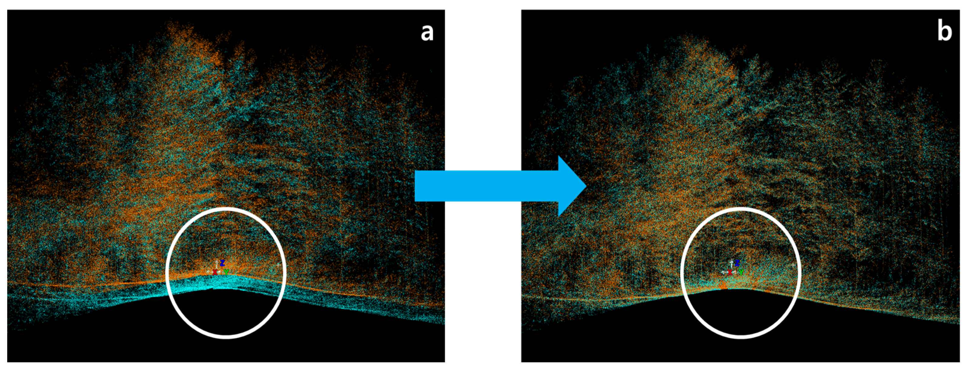
Unlike the BPLS, extracting forest variables from the TLS requires data preprocessing. The TLS scans each spot to co-register every spot’s point cloud. The automatic co-registration of the TLS Leica RTC360 tends to malfunction in forests with complicated topography or low radio waves. Thus, the Leica Cyclone REGISTER 360 software (Leica Geosystems, ST. Gallen, Switzerland) [42] was used to facilitate co-registration and improve the accuracy of the data (Figure 5).
Data collected from different scan spots were co-registered and integrated (Figure 5). The amount of time on co-registration increases with an increase in the number of scans. More concerning is that complicated topographies, such as a forest with a large amount of vegetation, are likely to cause occlusion, impeding data collection. This is likely to cause a reduction in the task efficiency. As the TLS obtains more point clouds and images over the same timeframe, it has larger data sets than the BPLS. A high-powered workstation was therefore used for the analysis. The workstation specifications were an AMD Ryzen Threadripper 3990X 2.9 GHz CPU, 256 GB RAM, NVIDIA GeForce RTX 2080 Ti*4 GPU, and a Windows 10 (64-bits) operating system.

2.4. Comparison of the Amount of Time Spent on Tasks for Efficiency Assessment

The labor required to examine forest resources was divided into office and field tasks. A group of three persons consisting of a recorder, a DBH measurer, and a height measurer conducted the field task. One person was required to use the TLS or BPLS. Table 4 summarizes all the office and field tasks required in each method. The amount of time spent on moving between spots and conducting multi-scans was included in the TLS processing time.

2.5. Statistical Analysis

The accuracy of each method was assessed by comparing height and DBH measurements between the three methods. The accuracy assessment for DBH and height was based on statistical values, including R2, RMSE, RMSE%, Bias, and Bias%. The R2 values ranged from 0 to 1. Values closer to 1 indicate larger correlations between dependent and independent variables. Higher values indicate that the regression model performs better. RMSE is a value used to assess accuracy by identifying differences between measurements and estimates. Bias is a value for the identification of the over- or underestimation of the estimates in relation to the measurements. Both values are commonly used to analyze a difference between an estimate and a measurement. The closer to zero the two values are, the better the model performs.
One-way analysis of variance (ANOVA) was utilized to identify the differences between the three methods. A post-hoc test [Tukeys’ honestly significant difference (HSD)] was conducted for factors that were statistically significant in the one-way ANOVA. The level of significance was within 5%. In addition, a paired t-test was applied. Measurements from the field survey were used as the reference values, and the data from the two LiDARs were used as the estimated values (Table 5).
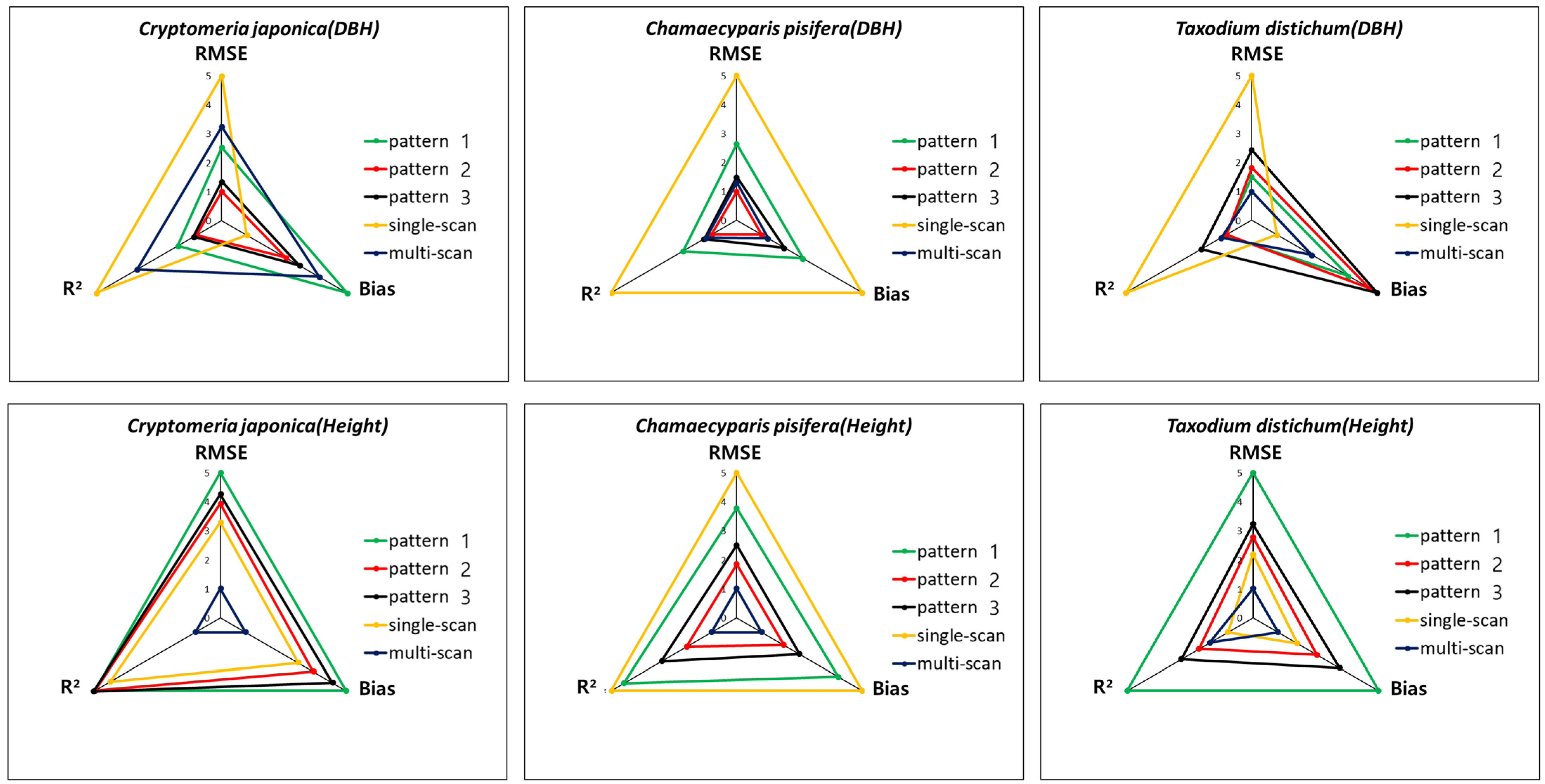
A traditional method of determining orders does not give the full explanation for the exact positions and orders between methods. Thus, in this study, relative orders were allocated to the statistical values of each method [43,44]. The relative positions were also marked. Optimal orders by the LiDAR and differences between methods were then suggested. The equation for analyzing the orders was as follows:
R i = 1 + m 1 × ( S i S m i n ) S m a x S m i n
where R i is the relative rank of equation i ( i = 1, 2, …, m), S i is the goodness-of-fit statistics produced by equation i , S m i n is the minimum value of the goodness-of-fit statistics, and S m a x is the maximum value of the goodness-of-fit statistics.
In the equation, values from 1 to m were considered as the highest and lowest orders, respectively, according to statistical criteria. In this study, a smaller triangle indicates a higher order. Bias% and RMSE% were excluded from the comparison because relative weighted values were already substituted, and they had the same tendencies as Bias and RMSE.

3. Results and Discussion

3.1. Stem Detection

The stem detection results drawn from the two LiDARs showed that there were 20, 26, and 7 standing trees in the Cryptomeria japonica, Chamaecyparis pisifera, and Taxodium distichum plots, respectively. The detection rates for both the BPLS and the TLS multi-scan method were 100%. In contrast, the detection rate of the TLS single-scan method was 95% (19 trees) in the Cryptomeria japonica plot and 88.46% (23 trees) in the Chamaecyparis pisifera plot, with four trees missed in total. The detection rate was 100% (seven trees) in the Taxodium distichum plot (Table 6).
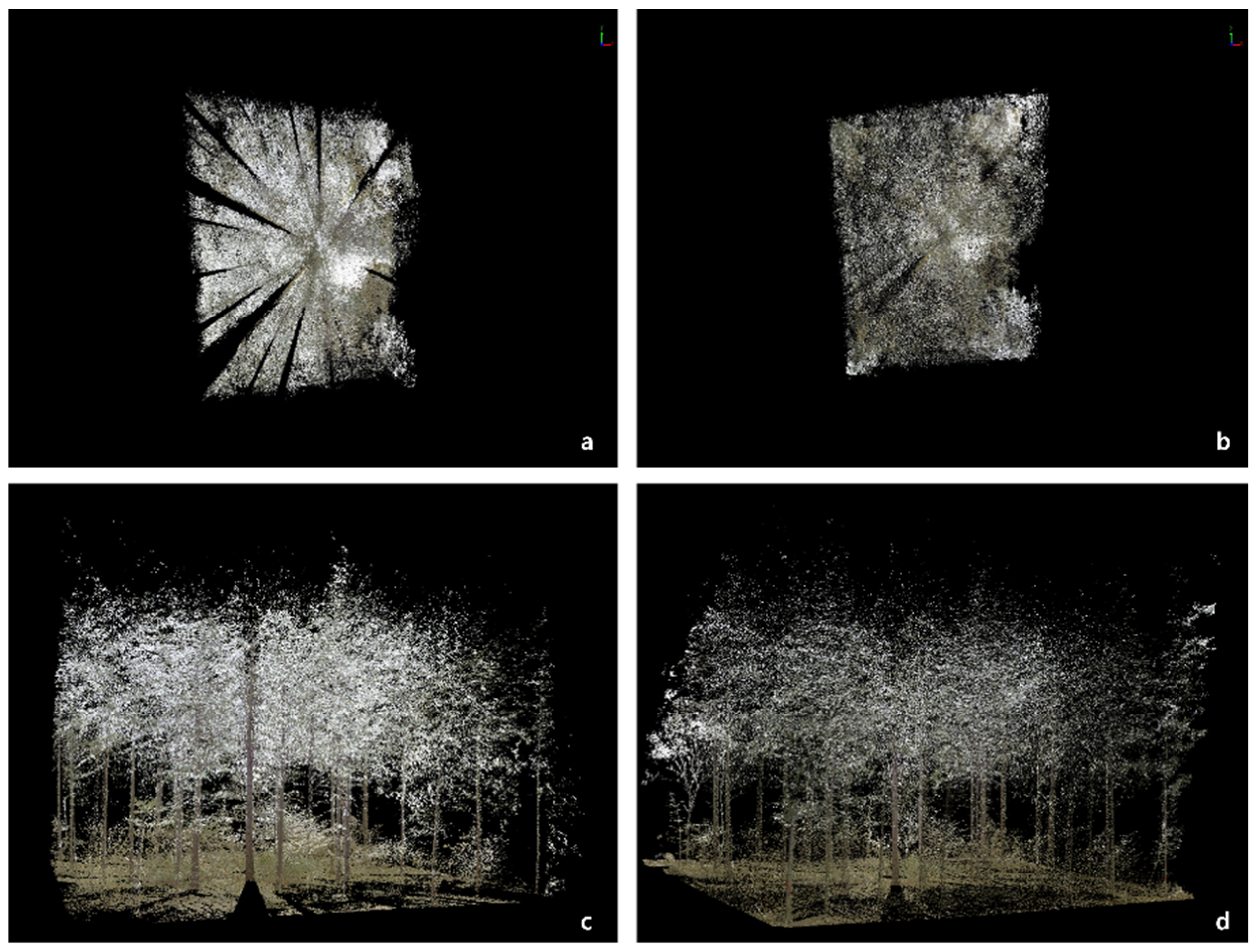
The perfect detection rate can be explained by high mobility. The researchers scanned all parts of each tree according to the three patterns, even in the sloped plot with high levels of vegetation, to avoid occlusion. However, the TLS was susceptible to occlusion. Corn-shaped occlusion caused by objects close to the TLS was an impediment to the full collection of point clouds with the TLS single-scan method, although all trees were detected using the TLS multi-scan method (Figure 6).
The occlusion issue with the single-scan method has also been identified in previous studies. For example, Shaobo et al. [44] showed that 157 of the 166 bamboo trees in a Chinese forest were detected using the single-scan method, thus achieving a detection rate of 88%. Likewise, the detection rate was 85% when Liang et al. [45] used the single-scan method to identify 44 of 52 Pinus sylvestris trees in Finland. One of the clear advantages of the TLS single-scan method is that data can be obtained rapidly. Nevertheless, the loss of point clouds caused by occlusion and the resultant low accuracy imply that the method is less applicable to the examination of forest resources. This flaw of the TLS single-scan method highlights one of the advantages of the BPLS. The detection rate of the BPLS was 100% even when scans were conducted only according to the border lines of the plot (Pattern 1; Figure 4). This suggests that the BPLS has a broader coverage and better control of occlusion effects than the TLS single-scan method. The two methods also differ in the accuracy and existence of their data. Nevertheless, more scans can eliminate the occlusion effect. The five scans in this study were sufficient to detect all trees in the three plots, indicating that it is necessary to scan at least five times.

3.2. Height and DBH Measurement Accuracy Assessment

Test statistics drawn from the comparison of height and DBH measurements between the two LiDARs and the field survey are shown in Table 7 and Figure 7. Liang et al. [46] found that the RMSE% value should be between 5% and 10% for a LiDAR device to be applicable to the estimation of forest resources. The RMSE% values of the TLS single-scan and the BPLS Pattern 1 were beyond this range. Therefore, the two methods are unsuitable for forest resource surveys. However, the bias values for the TLS single-scan method showed a larger goodness of fit than the other methods, particularly in the Cryptomeria japonica and Taxodium distichum plots. This can be explained by the differences between the reference and measurement values. The goodness of fit became larger as positive and negative values overlapped and converged to zero. Nevertheless, given all the other statistical indices, the single-scan method had the lowest goodness of fit, indicating its lower applicability to the examination of forest resources.
The results from the three plots show that the goodness of fit for DBH was larger for the BPLS than for the TLS, and the largest goodness of fit was found using Patterns 2 and 3. Additionally, the TLS multi-scan method showed a higher level of accuracy but a lower level of goodness of fit for the Cryptomeria japonica plot than for the other plots. A comparison of the differences between the three plots showed that the least accurate results were achieved in the Chamaecyparis pisifera plot because of its characteristics. The plot had more vegetation at around 1.2 m, which is the height up to which the stem is scanned to estimate DBH. Consequently, the targets were hidden, and this inhibited point cloud collection and reduced the accuracy of the TLS.
A more objective assessment of accuracy can be made by comparing the results to the existing literature. Bauwens et al. [1] assessed the applicability of using a TLS and a handheld mobile laser scanner (HMLS) to forest resource surveys. They reported RMSE and RMSE% values of 3.73 cm and 13.4% for a TLS single-scan method, 1.3 cm and 4.7% for a TLS multi-scan method, and 1.11 cm and 4.1% for the HMLS, respectively. As in this study, they also found that the TLS single-scan method had the lowest level of precision, while the HMLS was most accurate. Oveland et al. [47] compared the efficiency of a TLS, an HMLS, and a BPLS. Likewise, better performances were observed for the HMLS (RMSE: 3.1 cm, RMSE%: 14.3%) and BPLS (RMSE: 2.2 cm, RMSE%: 9.1%), whereas the TLS had an RMSE of 6.2 cm and RMSE% of 28.6%. Using a TLS and BPLS, Cabo et al. [17] measured DBH and vegetation height in two plots with different tree densities in an urban forest. The RMSE value for DBH was 0.011 cm in the plot with low tree density and 0.009 cm in the plot with high density, implying that there was a high level of accuracy. One of the main reasons for the high level of DBH accuracy in their study is that there was little vegetation at 1.3 m in the urban forest area, and thus, their analysis was not susceptible to occlusion. It can be concluded that vegetation or occlusion causes data loss and affects the accuracy of DBH measurements when using a terrestrial LiDAR. Therefore, a diversity of scanning patterns should be devised according to the environment of a forest to obtain accurate DBH data.
Unlike DBH, in this study, the TLS multi-scan method showed a greater goodness of fit for the height measurements than the BPLS. The BPLS Pattern 1 was least accurate. Additionally, DBH values were more accurate than height values. However, concerning the TLS, height measurements were more accurate than DBH, as the accuracy of the TLS is often affected by occlusion. Nevertheless, the TLS has a wider scan coverage and higher stability because the TLS is a more static device when collecting data than the BPLS. It is thus suggested that the TLS performs better than the BPLS when measuring height.
A comparison of the three plots indicated that accuracy was greater in the plot with the lowest tree density. In contrast, the height estimates were relatively inaccurate in the sloped plot that contained Cryptomeria japonica. However, all the plots had negative values of Bias and Bias%. This implies that values drawn from the BPLS and TLS were underestimated when compared to those from a vertex.
Some previous studies have found lower accuracies than those reported in this study. Liang et al. [48], for example, divided three forests into Easy, Moderate, and Hard based on tree density and degree of vegetation to assess the accuracy of measuring tree variables using a TLS multi-scan method. The average accuracy was lower than that of this study, given that the RMSE and RMSE% of the height measurements were 2.4–4.5 m and 12–23% for Easy, and 4.0–47.7 m and 28–57% for Hard. Similarly, utilizing a TLS and a portable laser scanner (PLS), Cabo et al. [17] compared the height and DBH in two plots with different tree densities in Spain. The findings revealed that the difference in RMSE values between the two devices was 1.34 m in the plot with a lower density and 9.44 m in the plot with a higher density. The difference in the values resulted from the differences between the devices and plot environments. These studies also demonstrate the huge effect that the environment of a plot has on the accuracy of measuring height using a TLS. This is because of occlusion that occurs with increased tree density, which impedes the point acquisition for tree tops. A terrestrial laser scanner tends to underestimate a tree’s height. The device also has limited coverage, depending on its specifications. Therefore, it is important to consider the peculiarities of a forest when choosing a device. Moreover, various ways of obtaining point clouds should be employed to avoid tree top occlusion and thus enhance accuracy.
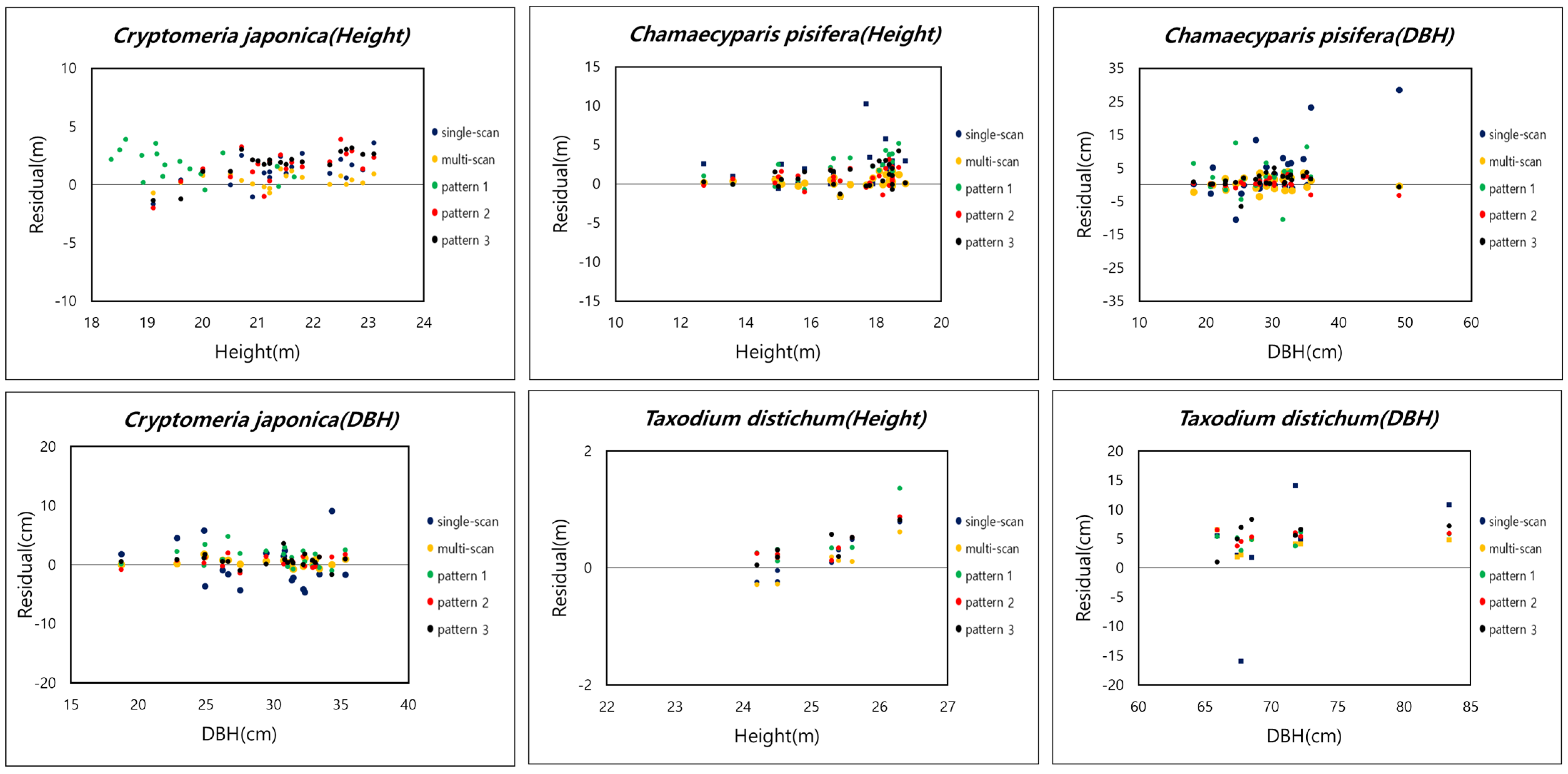
Residual errors were classified using height and DBH classes and then compared to analyze the trends of the BPLS and TLS measurements (Figure 8). The residual errors were calculated by using the differences in measurements between the field survey and LiDAR results. Values closer to zero indicate that they are closer to their reference values. The results showed that most of the residual errors were positive, implying an underestimation by the LiDAR. The trends in the residual errors of the two devices were similar in all plots. However, a high residual error range was found for height and DBH in the Chamaecyparis pisifera plot, but the residual error range was low in the Taxodium distichum plot. This difference is partly due to the larger tree density and more vegetation in the Chamaecyparis pisifera plot than in the other plots, both of which prevent the full acquisition of point clouds. In contrast, the Taxodium distichum plot with taller trees had more accurate height measurements, and this could be explained by the lower tree density.
As to height, a different trend in residual errors was identified only in Pattern 1 in the Cryptomeria japonica plot. This reveals that Pattern 1 with scans only according to the borderlines is less applicable to data collection. With regard to DBH, the TLS single-scan method caused large residual errors in all plots, indicating its tendency for under- and overestimation. The underestimation of residual errors was particularly clear in the Chamaecyparis pisifera plot. The large residual errors would be due to occlusion, preventing the TLS single-scan method from scanning all parts of a tree and reducing the accuracy.

3.3. Statistical Goodness of Fit for Each Method

One-way ANOVA was conducted to test the goodness of fit for each method (Table 8). For this, the results were compared between the field survey measurement and the multi-scan method using the TLS and the BPLS Pattern 2, as these showed the highest level of accuracy. Statistically significant differences between the three methods were not observed despite a clear difference in height measurements in the Cryptomeria japonica plot. Thus, a post-hoc test was conducted to identify the differences between the methods for height measurements of the plot. A statistically significant difference was found between the BPLS Pattern 2, the field survey, and the TLS multi-scan method (Table 9). The height measurements of the BPLS were more underestimated than those of the other two methods. This underestimation can be explained by a combination of the characteristics of the BPLS and environment of the Cryptomeria japonica plot. The plot had a slope of 24°, greater than that of the other plots. The accuracy was also affected by consistent movement of the BPLS, even in a highly sloped plot. The interaction between these two factors prevented the scanning of treetops, thus reducing accuracy. The measurements from the BPLS were thus underestimated compared to those from the TLS, which is a more static device. Further research is required to address the relatively lower performance of the BPLS in a sloped plot to increase the accuracy for data collection.
Additionally, paired t-test analyses were conducted to improve the identification of statistically significant differences between the two devices for each plot (Table 10). Statistically significant differences were found for height measurements in the Cryptomeria japonica plot and DBH measurements in the Taxodium distichum plot. A main reason for the statistically significant difference in height measurements in the Cryptomeria japonica plot is that the high slope of the plot prevented the BPLS from assessing the treetops. However, in the Taxodium distichum plot, irregular tree shapes led to differences in measurements between the BPLS and TLS.
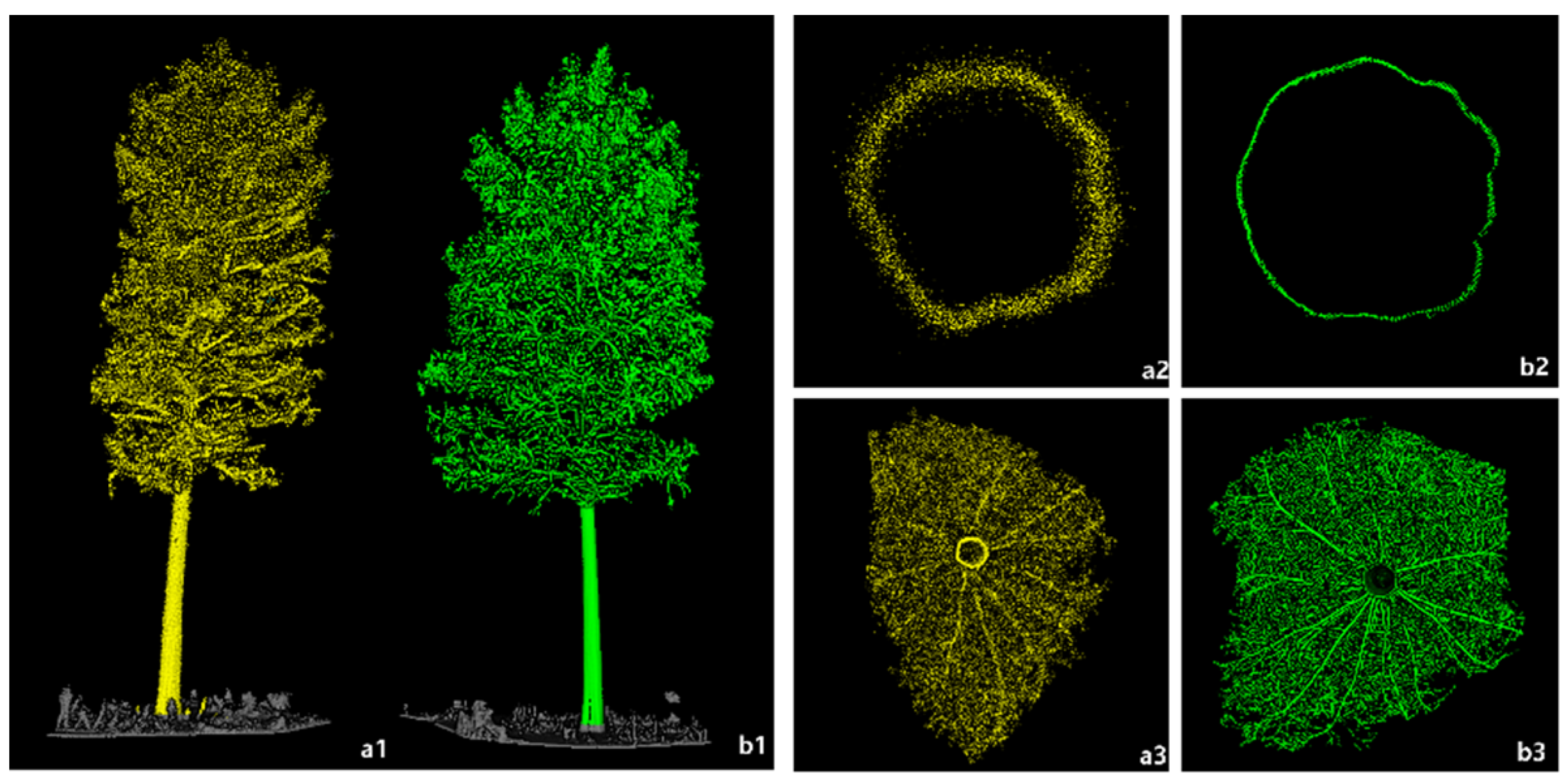
The TLS acquires 2 million points per second, and its scan accuracy is ±3 mm. However, the BPLS acquires 0.6 million points per second, and the accuracy is ±30 mm. Thus, it is natural that, in this study, the TLS had smaller residual errors and a higher density of point clouds than the BPLS (Figure 9). The difference in performances of the two devices becomes clear when identifying the point cloud density of the cross-section extracted from a tree at a height of 1.2 m. The density of the TLS was more intense than that of the BPLS, despite similar cross-section sizes. The BPLS would therefore cause a huge margin of error. It also turned out that the TLS was superior to the BPLS in the clear identification of branches. This shows the wide applicability of using a TLS for the estimation of the crown and branch biomass and management of protected and street trees, considering the angles and length of the branches.
The findings imply that the BPLS is less applicable to the collection of height and DBH data at millimeter levels, although appropriate for data collection at equal to or more than centimeter levels. This indicates that it is crucial to choose a device based on the purpose of the study and variables of interest.

3.4. Efficiency Assessment of the LiDAR Devices

The total amount of time spent completing all processes was recorded to compare the efficiency of tasks between the BPLS and TLS. The processes were then classified into office and field tasks. The amount of time spent extracting individual trees on a computer was also included in the office task. The results are shown in Table 11 and Table 12.
First, the BPLS field work results showed that the longer the pattern length, the more time it took to obtain the data. The amount of time was between 4.09 and 7.43 min for the Cryptomeria japonica plot, 3.95 and 7.15 min for the Chamaecyparis pisifera plot, and 2.97 and 5.91 min for the Taxodium distichum plot. A longer pattern also increased the number of point clouds, indicating a positive relationship between the two factors. As expected, Pattern 2 with the longest distance had the largest amount of data and took the longest time for all processes. However, the longest time does not necessarily mean the lowest efficiency. A comparison of the travel distances per hour shows that Pattern 2 was more efficient than the others. The Taxodium distichum plot was an exception as the travel distance of Pattern 2 was the longest under the same conditions. The Taxodium distichum plot was less dense than the other two plots, and Pattern 3 was the most efficient. Hence, the tree density of a plot is a crucial factor that determines which sampling pattern should be used.
The amount of time required to complete all office and field tasks with the TLS patterns is shown in Table 12. The time spent on each task ranged from 4.32 to 21.18 min for the Cryptomeria japonica plot, 4.55 to18.91 min for the Chamaecyparis pisifera plot, and 3.86 to 17.98 min for the Taxodium distichum plot. The TLS multi-scan method had the larger number of scans, and thus, it took longer than the TLS single-scan method. The TLS also obtained more data than the BPLS—2 million points per second for the TLS and 0.6 million points per second for the BPLS. Unlike the BPLS, the scanning time for the TLS increased with the increase in the number of scans. Therefore, the amount of time spent on processing the work increased with the increase in the number of scans.
The TLS single-scan method was not compared to the other methods in this study as it consisted of one scan at the center of the plot with no additional travel distances, discouraging a rational comparison. The travel distance per minute of the TLS multi-scan method was 0.31–0.47 m/min. The method was less efficient than the BPLS. Another efficiency comparison was made by calculating the area covered by a device per minute. The efficiency of the single-scan was 14.20–22.39 m2/min, whereas that of the multi-scan was 4.44–6.65 m2/min. However, no comparison of the two methods was made as it seemed unreasonable, given that the TLS needs more scans and takes longer time. The BPLS was more efficient than the TLS in all plots when comparing efficiency in terms of both distance and area covered per minute.
The efficiencies of the field survey and the TLS multi-scan method are shown in Table 13. The BPLS Pattern 2 was found to be the optimal method. The time spent on processing the work was 8.68–31.23 min for the field survey, 16.08–35.96 min for Pattern 2, and 60.13–90.14 min for the TLS. No clear differences were identified in the amount of time required between the field survey and BPLS in all the plots. As expected, the amount of time required for the TLS was high. Additionally, the amount of time required to cover 1 ha was measured by utilizing the amount of time spent on processing all the fieldwork. The findings showed that the amount of time was 164.5–678.3 min/ha for the field survey, 147.6–185.8 min/ha for the BPLS, and 449.5–529.5 min/ha for the TLS.
The efficiency of a field survey generally depends on the number of trees in a plot. This general tendency was also reflected in this study, causing a marked difference in the amount of time required to process the fieldwork. However, regarding the BPLS and TLS, office work had the largest impact on the total amount of time required. Unlike the BPLS, the TLS required more data processing time owing to the co-registration procedure for the different data collected at each scan spot (Figure 10). The co-registration procedure requires the largest share of labor when a forest is examined using the TLS. To improve the efficiency of co-registration, it is common to place conspicuous objects in forests or urban and indoor places. Nonetheless, the placement of objects did not enhance the efficiency in the study as the study sites were forests with complicated topographies. Thus, it is suggested that the TLS is less efficient when examining large forests.
The office work required for the field survey involves digitalizing written records. In contrast, using a LiDAR requires more steps, from preprocessing to extracting variables. In this study, the allocation of attribute values to point clouds accounted for a large portion of the entire procedure when using a LiDAR. The TLS also required more office work because of the co-registration before the analysis. The co-registration process is affected by the number of trees and environment of a plot, as it is carried out based on the appearance of point clouds. The amount of time also increases with an increase in the number of scans. This means that the time spent on the office work was much higher when using the LiDARs than when conducting the field survey. There are various ways of recording and storing the results of a forest resource inventory. Those in the traditional field survey method were handwritten and converted into Excel files. That is, all processes were conducted manually. The occurrence of errors is also inevitable when measuring and recording the tree variables. However, using a LiDAR can reduce errors considerably as it has a consistent algorithm to measure and record the tree variables irrespective of recorders or environments. The more accurate measurement of variables using a LiDAR will enhance the accuracy of estimations for tree volume, carbon sinks, biomass, and timber grades, and thus improve forest research and management. The efficiency in terms of the area covered by a surveyor per minute was also compared by plots. The BPLS was more efficient in the three plots than the TLS and field survey. The number of persons required for the field survey explained the lower efficiency of the field survey in this study as three surveyors were used to conduct it. Normally, at least three surveyors are required for a forest resource survey in South Korea. Thus, a decrease in the area covered per person is inevitable. The TLS was also less efficient than the other methods because more time was spent on scans and the office tasks to complete the co-registration.

4. Conclusions

This study assessed the applicability of terrestrial LiDARs for the examination of forest resource inventories and the construction of digital forest information. A BPLS and TLS were used to measure the height and DBH of trees in three different plots. The measurements were compared to those from a field survey to assess the efficiency of each method. The field survey is a traditional method to conduct forest resource inventories in which a caliper and diameter tape are used to measure the two tree variables. However, the traditional method has a clear limitation that it is impossible to acquire data for areas that surveyors cannot access. In contrast, laser scanning devices (LS) are relatively free from issues related to accessibility. These devices are operated manually, and their efficiency was low when they were first introduced. Nonetheless, the development of automatic estimation algorithms has led to more efficient and accurate data collection, and the widespread use of the LS devices. Additionally, they enable data to be obtained on tree variables, including the width and slope of the crown and slopes of branches, which is not possible with the traditional method. More importantly, LiDAR devices are also non-destructive and can thus be utilized to assess protected or inaccessible forests.
The two types of LiDARs have their own characteristics. The results of this study show that the BPLS is more efficient than the TLS and the field survey method when conducting a forest recourse inventory at a plot level. The higher efficiency of the BPLS is enabled by its ability to collect data for a large area in a shorter time. With regard to the patterns, Patterns 2 and 3 were most efficient as they covered the largest area in relation to the time despite their longer travel distances. Pattern 2 was efficient in the plot with the highest tree density, while Pattern 3 was also efficient in the plot with the lowest density. This study thus suggests that pattern selection should depend on the environment of a plot because LiDARs are sensitive to various forest conditions.
A LiDAR device generally acquires spatial information on objects by calculating the time taken by a laser pulse to go to an object and return to the device. Thus, in a dense plot with overlapped crowns of trees, data on top of the tree are not likely to be obtained fully, decreasing the accuracy of height measurements. It is therefore necessary to combine terrestrial and aerial LiDARs, such as a drone LiDAR, to obtain accurate height and crown estimates.
This study compared two LiDARs (i.e., LiBackpack D50 and RTC 360) to the traditional forest resource survey method. The results indicated that the use of LiDAR devices can be more efficient than traditional methods for data collection in terms of both cost and required workforce. This will facilitate forest management plans by providing accurate and timely information on forest resources. However, the efficiency and accuracy may vary according to the specifications of the LiDAR and computer. These limitations manifest themselves even more in South Korean forests that are complicated, mixed, and highly vegetated. The limitations are unlikely to be offset even by manual adjustments if the study area is vast. Thus, it is necessary to enhance algorithms and consider the environment of a forest when selecting a device. Future studies should examine the applicability and efficiency of LiDAR devices according to various environments.
This study suggests a more efficient method to acquire data that will be a basis for efficient forest management. The data can include timber yield and transactions, national forest management, thinning, and carbon sinks. A digital twin form of LiDAR data will enable longitudinal monitoring of forests and forest management activities and provide high quality reference data. The results of this study can also be used as basic data with which to design a manual for forest resource inventories and determine which device to utilize.

Author Contributions

Conceptualization, C.K. and D.K.; methodology, C.K.; software, C.K.; validation, C.K.; formal analysis, C.K.; investigation, C.K.; resources, J.L.; data curation, C.K. and J.L.; writing—original draft preparation, C.K.; writing—review and editing, C.K., J.L. and D.K.; visualization, C.K. and J.L.; supervision, C.K. and D.K.; project administration, J.K.; funding acquisition, J.K. All authors have read and agreed to the published version of the manuscript.

Funding

This research was funded by the National Institute of Forest Science, grant number FM0000-2020-01-2022.

Acknowledgments

This study was supported by the R&D Program for Forest Science Technology (Project No. FM0000-2020-01-2022) provided by the National Institute of Forest Science.

Conflicts of Interest

The authors declare no conflict of interest.

References

  1. Bauwens, S.; Bartholomeus, H.; Calders, K.; Lejeune, P. Forest inventory with terrestrial LiDAR: A comparison of static and hand-held mobile laser scanning. Forests 2016, 7, 127. [Google Scholar] [CrossRef] [Green Version]
  2. Hyyppä, E.; Kukko, A.; Kaijaluoto, R.; White, J.C.; Wulder, M.A.; Pyörälä, J.; Liang, X.; Yu, X.; Wang, Y.; Kaartinen, H.; et al. Accurate derivation of stem curve and volume using backpack mobile laser scanning. ISPRS J. Photogramm. Remote Sens. 2020, 161, 246–262. [Google Scholar] [CrossRef]
  3. Wang, Y.; Lehtomäki, M.; Liang, X.; Pyörälä, J.; Kukko, A.; Jaakkola, A.; Liu, J.; Feng, Z.; Chen, R.; Hyyppä, J. Is field-measured tree height as reliable as believed—A comparison study of tree height estimates from field measurement, airborne laser scanning and terrestrial laser scanning in a boreal forest. ISPRS J. Photogramm. Remote Sens. 2019, 147, 132–145. [Google Scholar] [CrossRef]
  4. Päivinen, R.; Merja, N.; Kari, T.K. Accuracy of certain tree measurements, Puutunnusten mittaamisen luotettavuus. Folia For. 1992, 787, 1–18. [Google Scholar]
  5. Kitahara, F.; Mizoue, N.; Yoshida, S. Effects of training for inexperienced surveyors on data quality of tree diameter and height measurements. Silva Fenn. 2010, 44, 657–667. [Google Scholar] [CrossRef] [Green Version]
  6. Rutzinger, M.; Kumar, A.P.; Oude Elberink, S.; Vosselman, G. Detection and modelling of 3d trees from mobile laser scanning data. Int. Arch. Photogramm. Remote Sens. Spat. Inf. Sci. 2010, 38, 520–525. [Google Scholar]
  7. Maltamo, M.; Næsset, E.; Vauhkonen, J. Forestry applications of airborne laser scanning. Concepts and Case Studies. Manag. For. Ecosys 2014, 27, 460. [Google Scholar]
  8. Chen, S.; Liu, H.; Feng, Z.; Shen, C.; Chen, P. Applicability of personal laser scanning in forestry inventory. PLoS ONE 2019, 14, e0211392. [Google Scholar] [CrossRef]
  9. Chambers, J.Q.; Asner, G.P.; Morton, D.C.; Anderson, L.O.; Saatchi, S.S.; Espírito-Santo, F.D.; Palace, M.; Souza Jr, C. Regional ecosystem structure and function: Ecological insights from remote sensing of tropical forests. Trends Ecol. Evol. 2007, 22, 414–423. [Google Scholar] [CrossRef]
  10. Næsset, E. Predicting forest stand characteristics with airborne scanning laser using a practical two-stage procedure and field data. Remote Sens. Environ. 2002, 80, 88–99. [Google Scholar] [CrossRef]
  11. Popescu, S.C.; Wynne, R.H.; Nelson, R.F. Measuring individual tree crown diameter with lidar and assessing its influence on estimating forest volume and biomass. Can. J. Remote Sens. 2003, 29, 564–577. [Google Scholar] [CrossRef]
  12. Næsset, E. Airborne laser scanning as a method in operational forest inventory: Status of accuracy assessments accomplished in Scandinavia. Scand. J. Forest Res. 2007, 22, 433–442. [Google Scholar] [CrossRef]
  13. Li, W.; Guo, Q.; Jakubowski, M.K.; Kelly, M. A new method for segmenting individual trees from the lidar point cloud. Photogramm. Eng. Remote Sens. 2012, 78, 75–84. [Google Scholar] [CrossRef]
  14. Vastaranta, M.; Wulder, M.A.; White, J.C.; Pekkarinen, A.; Tuominen, S.; Ginzler, C.; Kankare, V.; Holopainen, M.; Hyyppä, J.; Hyyppä, H. Airborne laser scanning and digital stereo imagery measures of forest structure: Comparative results and implications to forest mapping and inventory update. Can. J. Remote Sens. 2013, 39, 382–395. [Google Scholar] [CrossRef]
  15. Barrett, F.; McRoberts, R.E.; Tomppo, E.; Cienciala, E.; Waser, L.T. A questionnaire-based review of the operational use of remotely sensed data by national forest inventories. Remote Sens. Environ. 2016, 174, 279–289. [Google Scholar] [CrossRef]
  16. Cao, L.; Pan, J.; Li, R.; Li, J.; Li, Z. Integrating airborne LiDAR and optical data to estimate forest aboveground biomass in arid and semi-arid regions of China. Remote Sens. 2018, 10, 532. [Google Scholar] [CrossRef] [Green Version]
  17. Cabo, C.; Del Pozo, S.; Rodríguez-Gonzálvez, P.; Ordóñez, C.; González-Aguilera, D. Comparing terrestrial laser scanning (TLS) and wearable laser scanning (WLS) for individual tree modeling at plot level. Remote Sens. 2018, 10, 540. [Google Scholar] [CrossRef] [Green Version]
  18. Watt, P.J.; Donoghue, D.N.M. Measuring forest structure with terrestrial laser scanning. Int. J. Remote Sens. 2005, 26, 1437–1446. [Google Scholar] [CrossRef]
  19. Maas, H.G.; Bienert, A.; Scheller, S.; Keane, E. Automatic forest inventory parameter determination from terrestrial laser scanner data. Int. J. Remote Sens. 2008, 29, 1579–1593. [Google Scholar] [CrossRef]
  20. Moskal, L.M.; Zheng, G. Retrieving forest inventory variables with terrestrial laser scanning (TLS) in urban heterogeneous forest. Remote Sens. 2012, 4, 1–20. [Google Scholar] [CrossRef] [Green Version]
  21. Koreň, M.; Mokroš, M.; Bucha, T. Accuracy of tree diameter estimation from terrestrial laser scanning by circle-fitting methods. Int. J. Appl. Earth Obs. Geoinf. 2017, 63, 122–128. [Google Scholar] [CrossRef]
  22. Guan, H.; Su, Y.; Sun, X.; Xu, G.; Li, W.; Ma, Q.; Wu, X.; Wu, J.; Liu, L.; Guo, Q. A marker-free method for registering multi-scan terrestrial laser scanning data in forest environments. ISPRS J. Photogramm. 2020, 166, 82–94. [Google Scholar] [CrossRef]
  23. Liang, X.; Hyyppä, J. Automatic stem mapping by merging several terrestrial laser scans at the feature and decision levels. Sensors 2013, 13, 1614–1634. [Google Scholar] [CrossRef] [PubMed]
  24. Dassot, M.; Colin, A.; Santenoise, P.; Fournier, M.; Constant, T. Terrestrial laser scanning for measuring the solid wood volume, including branches, of adult standing trees in the forest environment. Comput. Electron. Agric. 2012, 89, 86–93. [Google Scholar] [CrossRef]
  25. Calders, K.; Newnham, G.; Burt, A.; Murphy, S.; Raumonen, P.; Herold, M.; Culvenor, D.; Avitabile, V.; Disney, M.; Armston, J.; et al. Nondestructive estimates of above-ground biomass using terrestrial laser scanning. Methods Ecol. Evol. 2015, 6, 198–208. [Google Scholar] [CrossRef]
  26. Kankare, V.; Holopainen, M.; Vastaranta, M.; Puttonen, E.; Yu, X.; Hyyppä, J.; Vaaja, M.; Hyyppä, H.; Alho, P. Individual tree biomass estimation using terrestrial laser scanning. ISPRS J. Photogramm. 2013, 75, 64–75. [Google Scholar] [CrossRef]
  27. Hackenberg, J.; Spiecker, H.; Calders, K.; Disney, M.; Raumonen, P. SimpleTree —An efficient open source tool to build tree models from TLS clouds. Forests 2015, 6, 4245–4294. [Google Scholar] [CrossRef]
  28. Lefsky, M.; McHale, M.R. Volume estimates of trees with complex architecture from terrestrial laser scanning. J. Appl. Remote Sens. 2008, 2, 023521. [Google Scholar]
  29. Huang, H.; Li, Z.; Gong, P.; Cheng, X.; Clinton, N.; Cao, C.; Ni, W.; Wang, L. Automated methods for measuring DBH and tree heights with a commercial scanning lidar. Photogramm. Eng. Remote Sens. 2011, 77, 219–227. [Google Scholar] [CrossRef]
  30. Hyyppä, E.; Xiaowei, Y.; Harri, K.; Teemu, H.; Antero, K.; Mikko, V.; Juha, H. Comparison of backpack, handheld, under-canopy UAV, and above-canopy UAV laser scanning for field reference data collection in boreal forests. Remote Sens. 2020, 12, 3327. [Google Scholar] [CrossRef]
  31. García, M.; Danson, F.M.; Riaño, D.; Chuvieco, E.; Ramirez, F.A.; Bandugula, V. Terrestrial laser scanning to estimate plot-level forest canopy fuel properties. Int. J. Appl. Earth Obs. Geoinf. 2011, 13, 636–645. [Google Scholar] [CrossRef]
  32. Kweon, H.K.; Seo, J.I.; Lee, J.W. Assessing the applicability of mobile laser scanning for mapping forest roads in the republic of Korea. Remote Sens. 2020, 12, 1502. [Google Scholar] [CrossRef]
  33. Saarela, S.; Johannes, B.; Pasi, R.; Anton, G.; Goran, S.; Mark, J.D.; Rasmus, A. Kriging prediction of stand-level forest information using mobile laser scanning data adjusted for nondetection. Can. J. For. Res. 2017, 47, 1257–1265. [Google Scholar] [CrossRef]
  34. Del Perugia, B.; Giannetti, F.; Chirici, G.; Travaglini, D. Influence of scan density on the estimation of single-tree attributes by hand-held mobile laser scanning. Forests 2019, 10, 277. [Google Scholar] [CrossRef]
  35. Ko, C.U.; Lee, S.H.; Yim, J.S.; Kim, D.G.; Kang, J.T. Comparison of forest inventory methods at plot-level between a backpack personal laser scanning (BPLS) and conventional equipment in Jeju Island, South Korea. Forests 2021, 12, 308. [Google Scholar] [CrossRef]
  36. The VL Vertex Laser. Available online: http://www.haglofcg.com/index.php/en/files/leaflets/46-vl5-product-sheet (accessed on 8 September 2022).
  37. Leica. Leica RTC360 3D Reality Capture Solution. 2022. Available online: https://leica-geosystems.com/products/laser-scanners/scanners/leica-rtc360 (accessed on 8 September 2022).
  38. LiBackpack. Mobile Handheld LiDAR—3D Mapping System. Available online: https://greenvalleyintl.com/hardware/libackpack/ (accessed on 8 September 2022).
  39. Tao, S.; Wu, F.; Guo, Q.; Wang, Y.; Li, W.; Xue, B.; Hu, X.; Li, P.; Tian, D.; Li, C.; et al. Segmenting tree crowns from terrestrial and mobile LiDAR data by exploring ecological theories. ISPRS J. Photogramm. 2015, 110, 66–76. [Google Scholar] [CrossRef] [Green Version]
  40. LiDAR360—Point Cloud Processing Software. Available online: https://greenvalleyintl.com/software/lidar360/ (accessed on 8 September 2022).
  41. Poudel, K.P.; Cao, Q.V. Evaluation of methods to predict weibull parameters for characterizing diameter distributions. Forest Sci. 2013, 59, 243–252. [Google Scholar] [CrossRef]
  42. Leica. Leica Cyclone 3D Point Cloud Processing Software. 2022. Available online: https://leica-geosystems.com/products/laser-scanners/software/leica-cyclone (accessed on 8 September 2022).
  43. Doyog, N.D.; Lee, Y.J.; Lee, S. Stem taper equation analysis for Larix kaempferi species in the central region of South Korea. J. Sustain. For. 2017, 36, 747–763. [Google Scholar] [CrossRef]
  44. Xia, S.; Wang, C.; Pan, F.; Xi, X.; Zeng, H.; Liu, H. Detecting stems in dense and homogeneous forest using single-scan TLS. Forests 2015, 6, 3923–3945. [Google Scholar] [CrossRef] [Green Version]
  45. Liang, X.; Hyyppä, J.; Kankare, V.; Holopainen, M. Automatic plot-wise tree location mapping using single-scan terrestrial laser scanning. Photogramm. J. Finl. 2011, 22, 37–48. [Google Scholar]
  46. Liang, X.; Wang, Y.; Pyörälä, J.; Lehtomäki, M.; Yu, X.; Kaartinen, H.; Kukko, A.; Honkavaara, E.; Issaoui, A.E.I.; Nevalainen, O.; et al. Forest in situ observations using unmanned aerial vehicle as an alternative of terrestrial measurements. For. Ecosyst. 2019, 6, 20. [Google Scholar] [CrossRef] [Green Version]
  47. Oveland, I.; Marius, H.; Francesca, G.; Narve Schipper, K.; Terje, G. Comparing three different ground based laser scanning methods for tree stem detection. Remote Sens. 2018, 10, 538. [Google Scholar] [CrossRef] [Green Version]
  48. Liang, X.; Hyyppä, J.; Kaartinen, H.; Lehtomäki, M.; Pyörälä, J.; Pfeifer, N.; Holopainen, M.; Brolly, G.; Francesco, P.; Hackenberg, J. International benchmarking of terrestrial laser scanning approaches for forest inventories. ISPRS J. Photogr. Remote Sens. 2018, 144, 137–179. [Google Scholar] [CrossRef]
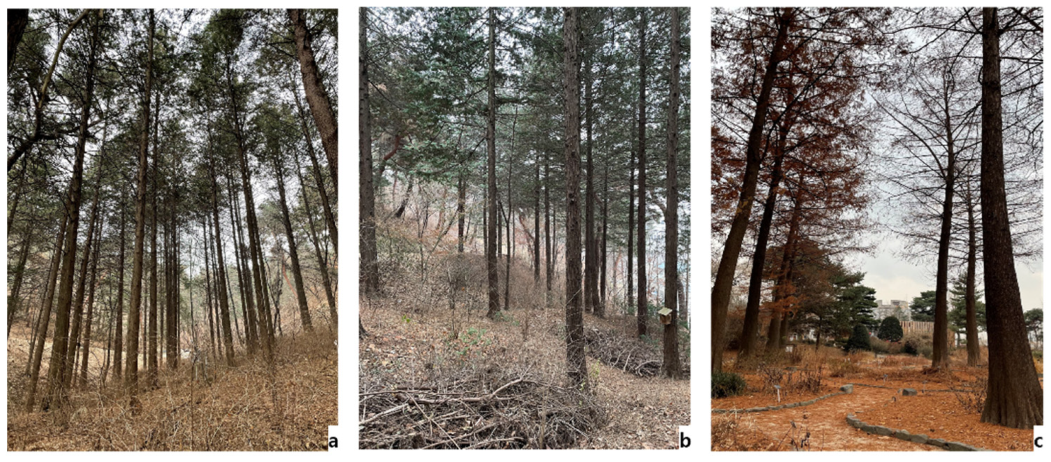
Figure 1. Landscapes of the study area. (a) Cryptomeria japonica, (b) Chamaecyparis pisifera, and (c) Taxodium distichum.
Forests 13 02087 g001
Figure 2. Photographs of the survey using (a) Vertex Laser Geo, (b) LiBackpack D50, and (c) RTC360.
Forests 13 02087 g002
Figure 3. Data collection using TLS (a) single-scan and (b) multi-scan.
Forests 13 02087 g003
Figure 4. Data collection using BPLS (a) Pattern 1, (b) Pattern 2, and (c) Pattern 3.
Forests 13 02087 g004
Figure 5. Description of the co-registration procedure using the software, Cyclone REGISTER 360. (a) before co-registration and (b) after co-registration.
Forests 13 02087 g005
Figure 6. Comparison of the single- and multi-scan TLS showing the occlusion effect. (a,c) are examples of the corn-shaped occlusion that hindered the single-scan method, while (b,d) show that the corn-shaped occlusion was controlled by the multi-scan method to obtain all point clouds.
Forests 13 02087 g006
Figure 7. Rankings by statistical accuracy.
Forests 13 02087 g007
Figure 8. Comparison of the residual errors for height and DBH class using the TLS and BPLS.
Forests 13 02087 g008
Figure 9. Comparison of data results between two devices for the same tree. Tree scanned using (a1) BPLS and (b1) TLS. Cross-section at breast height using (a2) BPLS and (b2) TLS. Bottom view of a standing tree using (a3) BPLS and (b3) TLS.
Forests 13 02087 g009
Figure 10. Comparison of the share of each internal task of the entire process by device and species.
Forests 13 02087 g010
Table 1. Geographical characteristics of each plot in the study area.
Plot SpeciesPlot Size
(ha)
Altitude
(m)
Slope
(°)
Wind Speed (m/s)
Cryptomeria japonica0.0465243
Chamaecyparis pisifera0.043783
Taxodium distichum0.044003
Table 2. Description of the TLS (RTC360) and the BPLS (LiBackpack D50).
Specifications
Laser SensorTLS (Leica RTC360)BPLS (Velodyne VLP-16*2)
Wavelength1550 nm905 nm
LiDAR Accuracy1.9–5.3 mm
(1.9 mm @ 10 m
2.9 mm @ 20 m
5.3 mm @ 40 m)
±3 cm
Scan Range130 m100 m
Weight5.35 kg without battery8.8 kg without battery
Scan Rate2,000,000 pts/s600,000 pts/s
Field of viewvertical: 300°
horizonal: 360°
vertical: −90°–+90°
horizonal: 360°
Camera36 MP 3-camera system
432 MPx raw data for calibrated 360° × 300° spherical image
Table 3. Summary statistics for the sample trees in each sample plot.
Plot No.Number of TreesStem Density
(Trees/ha)
DBH (cm)Tree Height (m)Basal Area
(m2/ha)
MeanStd.MinMaxMeanStd.MinMaxMeanStd.
Cryptomeria japonica2050029.34.1418.734.321.691.019.623.134.40.29
Chamaecyparis pisifera2665029.36.2018.149.117.051.7012.718.945.60.34
Taxodium distichum717571.05.9465.983.425.91.102427.369.640.85
Table 4. Survey method categorization by device.
Survey MethodTotal Time Elapsed
Field WorkOffice Work
Traditional field surveyPlot extraction,
height estimation, DBH estimation
Digitization of field measurement
BPLSPlot extraction
Point cloud acquisition
Variable extraction using point cloud
TLSPlot extraction
Point cloud acquisition
Co-registration
Variable extraction using point cloud
Table 5. Statistical accuracy of the BPLS, TLS, and field survey.
StatisticsCalculation Forms
Coefficient   of   determination   ( R 2 ) 1 ( x i x ^ i ) 2 ( x i x ¯ i ) 2
Bias i = 1 n ( x i x i ^ ) / n
Bias% B i a s x i ¯ × 100 %
Root Mean Square Error (RMSE) i = 1 n x i x i ^ 2 n
Root Mean Square Error% (RMSE%) R M S E x i ¯ × 100 %
where x i , x i ^ ,   a n d   x i ¯ = a reference value (field survey), an estimated value (LiDAR), and the mean of a reference value, respectively. n = the number of trees.
Table 6. Accuracy of tree mapping using the BPLS and TLS data.
Study SiteReferenceMappedPercentage (%)
BPLS
(Pattern 1)
Cryptomeria japonica2020100
Chamaecyparis pisifera2626100
Taxodium distichum77100
BPLS
(Pattern 2)
Cryptomeria japonica2020100
Chamaecyparis pisifera2626100
Taxodium distichum77100
BPLS
(Pattern 3)
Cryptomeria japonica2020100
Chamaecyparis pisifera2626100
Taxodium distichum77100
TLS
(single-scan)
Cryptomeria japonica201995
Chamaecyparis pisifera262388.46
Taxodium distichum77100
TLS
(multi-scan)
Cryptomeria japonica2020100
Chamaecyparis pisifera2626100
Taxodium distichum77100
Table 7. Comparative accuracy assessment of the obtained DBH and vegetation height data using the BPLS and TLS by pattern.
Study SiteStatisticDBH (cm)Height (m)
Pattern 1Pattern 2Pattern 3Single-scanMulti-scanPattern 1Pattern 2Pattern 3Single-scanMulti-scan
Cryptomeria japonicaRMSE1.991.021.243.572.452.492.032.171.750.76
RMSE%6.753.464.2012.118.3011.639.4910.138.203.58
Bias−1.29−0.52−0.68−0.03−0.94−2.04−1.51−1.82−1.27−0.42
Bias%−4.38−1.76−2.32−0.10−3.19−9.55−7.04−8.51−5.93−1.95
0.900.960.950.640.770.040.040.030.140.70
Chamaecyparis pisiferaRMSE4.801.502.499.542.102.391.271.653.100.78
RMSE%16.405.118.5032.597.1814.027.449.7018.204.55
Bias−2.12−0.40−1.34−4.58−0.66−1.70−0.76−1.03−2.08−0.38
Bias%−7.22−1.35−4.56−15.65−2.25−10.0−4.45−6.02−12.18−2.20
0.680.950.880.0030.900.280.680.520.20.84
Taxodium distichumRMSE5.05.416.209.524.350.580.430.460.390.31
RMSE%7.047.628.7413.416.132.331.721.811.561.21
Bias−4.89−5.34−5.51−3.33−4.09−0.41−0.22−0.29−0.16−0.10
Bias%−6.88−7.53−7.77−4.69−5.76−1.62−0.88−1.16−0.65−0.40
0.970.980.740.020.930.660.860.810.940.89
Table 8. Results of one-way ANOVA analysis by device.
Study SiteVariableSum of SquaresMean SquareFp-Value
Cryptomeria japonicaHeight24.1912.099.59<0.005
DBH21.9010.950.560.57
Chamaecyparis pisiferaHeight7.463.731.240.30
DBH5.702.850.070.93
Taxodium distichumHeight0.170.080.260.77
DBH109.2454.621.590.23
Table 9. Post-hoc results of height for Cryptomeria japonica.
Study SiteEquipmentMeanTukey Grouping
Cryptomeria japonicaVertex21.39A
TLS20.97A
BPLS19.88B
Table 10. Paired t-test analysis using the TLS and BPLS data.
Study SiteVariableEquipmentNumber of TreesMeanS.D.S.E.t ValuePr > |t|
Cryptomeria japonicaHeightTLS (multi-scan)2020.971.371.174.00<0.005
BPLS (Pattern 2)19.881.211.10
DBHTLS (multi-scan)30.4223.034.802.790.011
BPLS (Pattern 2)28.9617.204.15
Chamaecyparis pisiferaHeightTLS (multi-scan)2616.672.891.701.970.059
BPLS (Pattern 2)16.293.291.81
DBHTLS (multi-scan)28.6238.456.20−0.650.523
BPLS (Pattern 2)28.8844.146.64
Taxodium distichumHeightTLS (multi-scan)725.010.270.521.800.121
BPLS (Pattern 2)24.890.160.40
DBHTLS (multi-scan)66.9035.125.933.86<0.005
BPLS (Pattern 2)65.6432.845.73
Table 11. Comparison of the amount of time required to gather and process data with the BPLS according to scan patterns.
Study
Site
PatternArea
[m²]
Travel
Distance
[m]
Time Consumption [min]Total Point Cloud [n]Efficiency by the Distance Covered per Minute
[m/min]
Survey
[min]
Processing
[min]
Total
Times
[min]
(A)(B) (C) (D) = (B)/(C)
Cryptomeria japonica1400804.0914.4718.575,959,489 4.31
22007.4325.0632.5014,062,705 6.15
31606.0522.7028.7512,198,763 5.57
Chamaecyparis pisifera1803.9516.0219.977,295,071 4.01
22007.1528.8135.9619,135,965 5.56
31606.4328.2534.6713,402,931 4.61
Taxodium distichum1802.976.469.433,407,910 8.48
22005.9110.1716.087,157,977 12.44
31604.847.3212.144,946,240 13.17
Table 12. Comparison of the amount of time required to gather and process the data with the TLS according to scan patterns.
Study
Site
PatternArea
[m²]
Travel
Distance
[m]
Time [min]Total Point Cloud [n]Efficiency as the Distance Covered per Minute
[m/min]
Efficiency as the Area Covered per Minute
[m²/min]
Survey
[min]
Processing
[min]
Total
Times
[min]
(A)(B) (C) (D) = (B)/(C)(E) = (A)/(C)
Cryptomeria japonicasingle
scan
40004.3221.0225.3423,558,038 0.0015.78
multi
scan
28.321.1868.9690.1470,306,600 0.314.44
Chamaecyparis pisiferasingle
scan
04.5523.6228.1624,399,432 0.0014.20
multi
scan
28.318.9165.9384.8452,962,020 0.334.71
Taxodium distichumsingle
scan
03.8614.0017.8721,230,763 0.0022.39
multi
scan
28.317.9842.1660.1360,482,287 0.476.65
Table 13. Comparison of efficiencies for the BPLS, TLS and field survey.
Study
Site
Survey MethodPersonnelArea
(m²)
Time Consumption [min]Survey Coverage per Surveyor
(m²/min)
Outdoor
Task
Indoor TaskTotal
Co-RegistrationProcessing
Cryptomeria japonicaField survey340016.9803.2720.256.58
BPLS(Pattern 2)17.433025.0632.5012.31
TLS(multi-scan)121.183028.9690.144.44
Chamaecyparis pisiferaField survey327.1304.131.234.27
BPLS(Pattern 2)17.148028.8135.9611.12
TLS(multi-scan)118.912540.9384.844.71
Taxodium distichumField survey36.5802.18.6815.36
BPLS(Pattern 2)15.905010.1716.0824.88
TLS(multi-scan)117.981527.1560.136.65
Publisher’s Note: MDPI stays neutral with regard to jurisdictional claims in published maps and institutional affiliations.