Article

Study on the Moisture Content Diagnosis Method of Living Trees Based on WASN and CTWGAN-GP-L

College of Information Science and Technology, Nanjing Forestry University, Nanjing 210037, China
*
Author to whom correspondence should be addressed.
Forests 2022, 13(11), 1879; https://doi.org/10.3390/f13111879
Submission received: 15 September 2022 / Revised: 2 November 2022 / Accepted: 5 November 2022 / Published: 9 November 2022
(This article belongs to the Special Issue Advances in Forest Fire and Other Detection Systems)

Abstract

:
Water is an important component of tree cells, so the study of moisture content diagnostic methods for live standing trees not only provides help for production management in agriculture, forestry and animal husbandry but also provides technical guidance for plant physiology. With the booming development of deep learning in recent years, the generative adversarial network (GAN) provides a method to solve the problem of insufficient manual sample collection and tedious and time-consuming labeling. In this paper, we design and implement a wireless acoustic sensor network (WASN)-based wood moisture content diagnosis system with the main objective of nondestructively detecting the water content of live tree trunks. Firstly, the WASN nodes sample the acoustic emission signals of tree trunk bark at high speed then calculate the characteristic parameters and transmit them wirelessly to the gateway; secondly, the Conditional Tabular Wasserstein GAN-Gradient Penalty-L (CTWGAN-GP-L) algorithm is used to expand the 900 sets of offline samples to 1800 sets of feature parameters to improve the recognition accuracy of the model, and the quality of the generated data is also evaluated using various evaluation metrics. Moreover, the optimal combination of features is selected from the expanded mixed data set by the random forest algorithm, and the moisture content recognition model is established by the LightGBM algorithm (GSCV-LGB) optimized by the grid search and cross-validation algorithm; finally, real-time long-term online monitoring and diagnosis can be performed. The system was tested on six tree species: Magnolia (Magnoliaceae), Zelkova (Ulmaceae), Triangle Maple (Aceraceae), Zhejiang Nan (Lauraceae), Ginkgo (Ginkgoaceae), and Yunnan Pine (Pinaceae). The results showed that the diagnostic accuracy was at least 97.4%, and the designed WASN model is fully capable of long-term deployment for observing tree transpiration.

1. Introduction

Drought is known to have profound effects on forest health, as evidenced by several severe events in recent decades. Extensive forest mortality due to drought can impair the ecological functions of forests; affect forest habitats, water production, and quality; and alter the dynamics and intensity of forest fires [1]. However, changes in moisture content within living trees are usually not accessible through direct observation. Therefore, this paper addresses the need for tree water physiological measurement and the development of forestry information technology and uses a combination of the wireless acoustic sensor network (WASN) and Conditional Tabular Wasserstein GAN-Gradient Penalty-L (CTWGAN-GP-L) to diagnose and study the moisture content of live standing trees, which is important for the development and promotion of forestry Internet of Things in China.
Regarding the measurement of wood moisture content, many methods have been proposed by domestic and foreign scholars, such as the oven-drying method, electrical resistance method, and nuclear magnetic resonance method [2,3,4]. The measuring accuracy of the oven-drying method is the highest, but the measuring process is complicated and destructive. The resistance method is one of the earliest measurement methods in electrical measurement, but the accuracy is not high when the Moisture Content (MC) is above 30%. The nuclear magnetic resonance method is costly and not easy to operate in the field. In recent years, with the development of Nondestructive Testing (NDT) technology, time-domain reflectometry, the capacitance method and Near Infrared (NIR) spectroscopy have received more attention: Joseph Dahlen et al. used time-domain reflectometry to analyze and model the moisture content of wood [5]; Vu Thi Hong Tham and Tetsuya Inagaki et al. studied wood moisture content combining capacitance and NIR spectroscopy, a new method for estimation [6]; and Luana Maria dos Santos and Evelize Aparecida Amaral et al. developed a NIR spectral model to estimate the moisture content in wood samples [7]. Although the capacitance and NIR spectroscopy methods are widely used, they still have disadvantages such as difficulty in modeling and poor sensitivity.
In addition, the acoustic emission (AE) signal characteristics of wood with different moisture contents have received continuous attention: Xinci Li et al. investigated the effect of the moisture content on the acoustic emission signal propagation characteristics of Sargassum pine [8]; Vahid Nasir et al. used AE sensors and accelerometers to detect stress waves in thermally modified woods and explored the effect of heat treatment on wave velocity and AE signal, and used machine learning methods to classify and evaluate its moisture content [9]. These studies show that differences in the moisture content of trees can lead to significant changes in their AE signal characteristics, but no studies based on AE signal inversion of the moisture content have been reported. In addition, Yong Wang et al. used deep learning (DL) to predict the wood moisture content [10], Debapriya Hazra et al. used Wasserstein GAN-Gradient Penalty-Acxiliary Classifier (WGAN-GP-AC) to generate synthetic microscopic cell images to improve the classification accuracy of each cell type [11], and Hongwei Fan et al. used Local Binary Pattern (LBP) to convert vibration signals into grayscale texture images and then used Wasserstein GAN-Gradient Penalty (WGAN-GP) to expand the data for grayscale texture images [12]. Liang Ye et al. used CTGAN to generate 3D images of the mandible with different levels and rich morphology on six mandibular tumor case datasets [13]; Jinyin Chen et al. used Conditional Tabular GAN (CTGAN) to generate various textual contents with variable lengths [14], but no one has yet combined Conditional GAN (CGAN), WGAN-GP with L regularization to form the CTWGAN-GP-L algorithm and used it to expand the processing study on tabular data, let alone combining WASN with CTWGAN-GP-L to accurately measure the moisture content of living trees in real time.
In this paper, we conducted the first study of WASN and CTWGAN-GP-L based on the diagnosis of the moisture content of live standing trees: we used a self-designed low-power and high-precision WASN node, which can collect AE signals at a sampling rate of 5 Million samples per second (Msps), then calculate the feature parameters and transmit them wirelessly to the gateway, and then expand the collected 900 sets of offline sample feature parameter data to 1800 sets using the CTWGAN-GP-L algorithm. Moreover, we use the CTWGAN-GP-L algorithm to expand the collected 900 sets of offline samples to 1800 sets to improve the recognition accuracy of the model; also, the quality of the generated data is evaluated using various evaluation metrics. Furthermore, the optimal combination of features is selected from the expanded mixed data set by the random forest algorithm, and the moisture content recognition model is established by the LightGBM algorithm (GSCV-LGB) optimized by the grid search and cross-validation algorithm; finally, real-time long-term online monitoring and diagnosis can be performed. The system was tested on magnolia, zhejiang nan, camphor maple, triangle maple, ginkgo tree and balsam fir trees at Nanjing Forestry University, and the test results proved that its diagnostic recognition rate could reach 98.1%, which fully met the requirements of long-term deployment in the forestry field.

2. Materials and Methods

2.1. System Architecture Framework

Since the forestry Internet of Thing (IoT) is developing in a more refined way, this will undoubtedly drive and advance the development of a large number of low-cost sensor nodes and wireless communication. Sensors with data-processing capability are placed in the air, tree trunk, or its root soil to automatically monitor and collect the temperature, humidity, nutrients, wind direction, wind, depression, and moisture content and automatically process these signals on the network. The basic architecture of a forestry IoT system is shown in Figure 1. However, the actual deployment of WSN nodes faces many difficulties, such as the lack of wide network coverage, relatively high infrastructure costs, short node battery life, and high energy consumption. Therefore, Long Range(LoRa)technology, which can provide low power consumption and remote wireless transmission, has been widely used.

2.2. Wireless Acoustic Emission Sensing Node Design

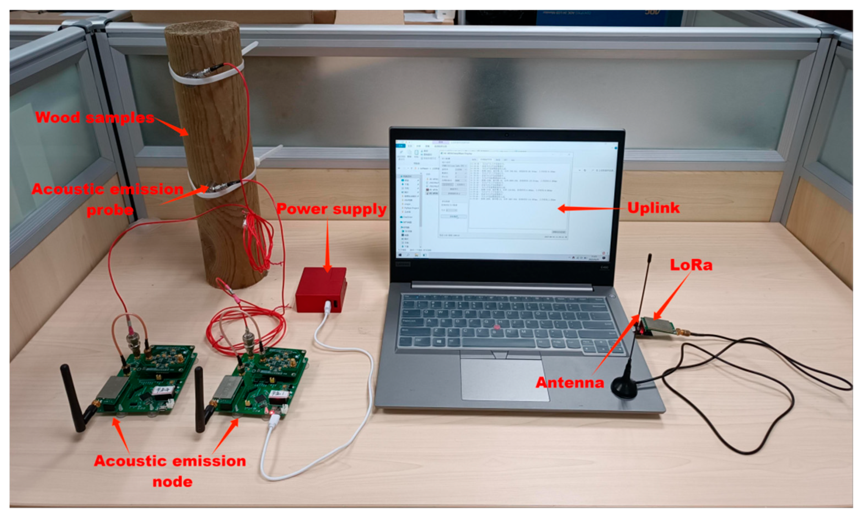
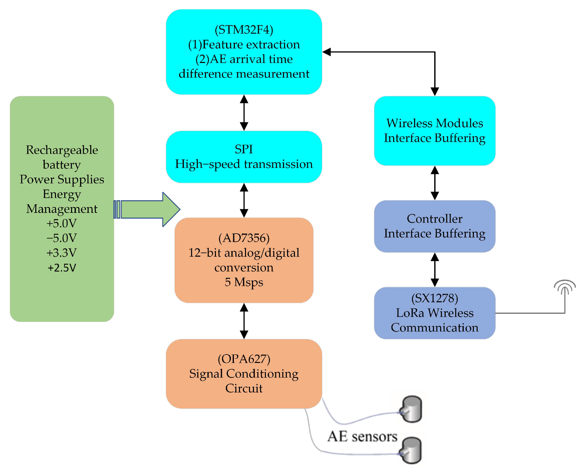
The WASN node used in this paper uses the UT-1000 acoustic emission sensor (MISTRAS Group, Inc., Princeton Jct, NJ, USA) of American Physical Acoustics to collect the acoustic emission signal of wood samples, and through the OPA627 operational amplifier chip (Texas Instruments Inc., Dallas, TX, USA), the acoustic emission raw signal is amplified and processed, then the AD7356 chip (Analog Devices, Inc., Norwood, MA, USA) is used to convert the acoustic emission signal analog to digital. Furthermore, the acoustic emission signal is read by the STM32F405RG chip (STMicroelectronics, Geneva, Switzerland) based on the Cotex-M4 core. Finally, after data pre-processing and data storage, the acoustic emission signal data are sent to the gateway via the SX1278-based LoRa module (SEMTECH Corporation, Camarillo, CA, USA). The composition and interconnection of each module of the node are shown in Figure 2, and the physical sample and installation measurement example are shown in Figure 3.
The sound source in the data-acquisition process is generated by a micro-vibration motor fixed on the tree trunk, and the stress waves emitted during the test are propagated through the surface of the trunk and thus collected by the AE sensor immediately adjacent to the tree bark; to enhance the system’s anti-interference capability, two R15α-type probes are selected to be deployed longitudinally at 20 cm intervals near the tree diameter at breast height (1.4 m above ground), and the sound source is placed vertically in a three-point line on the upper side of the two probes, 10 cm apart from the proximal probe. In this way, the AE signals of the distant and near probes can be calculated as a difference to reduce the system measurement error as much as possible.

2.3. AE Data Acquisition

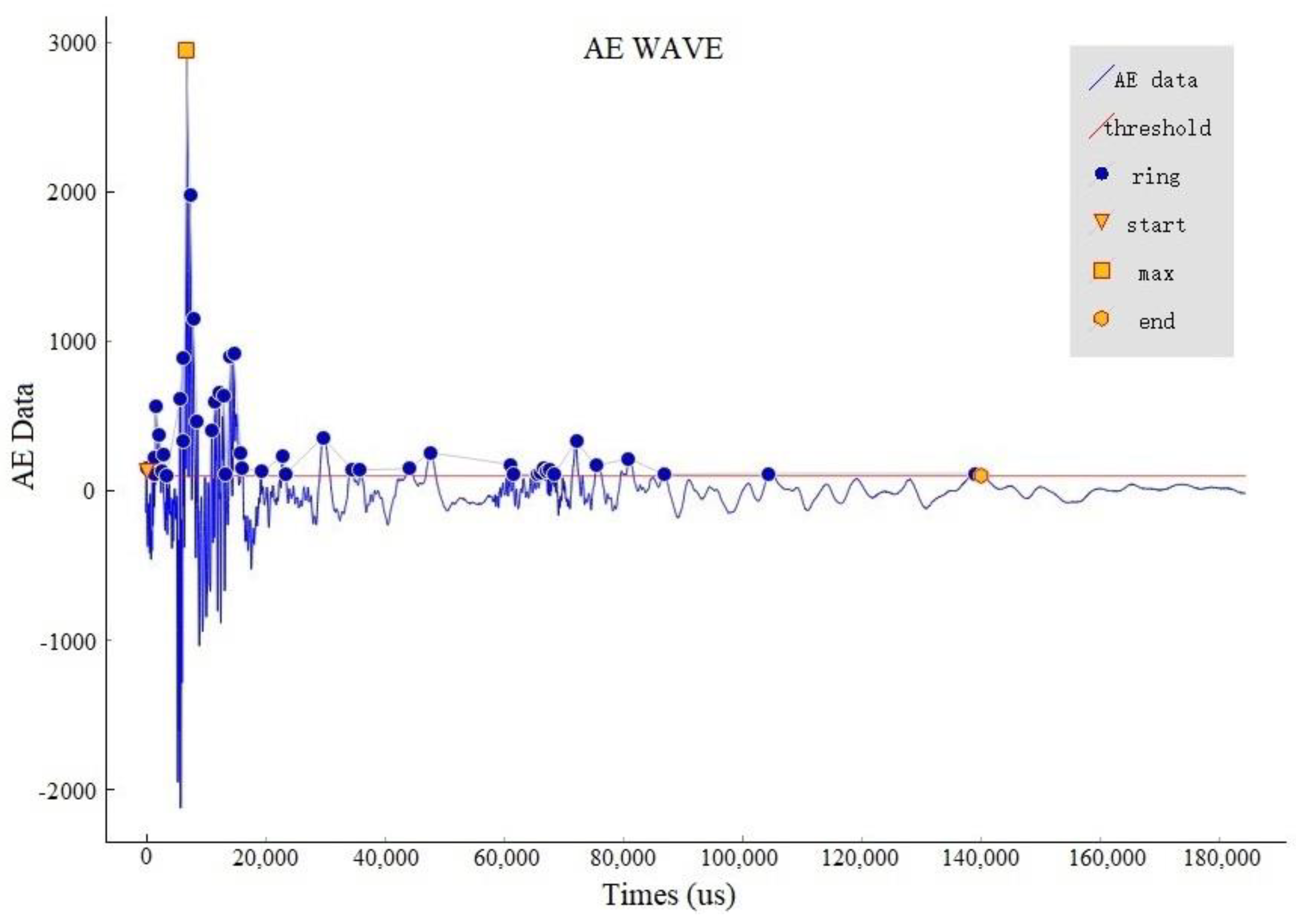
The AE data collected by all WASN nodes can be sent to the gateway for aggregation and display, and the collection curve is shown in Figure 4. Each characteristic parameter (amplitude, rise time, duration, ringing count, and energy) is then used to construct the data sample set for moisture content determination.
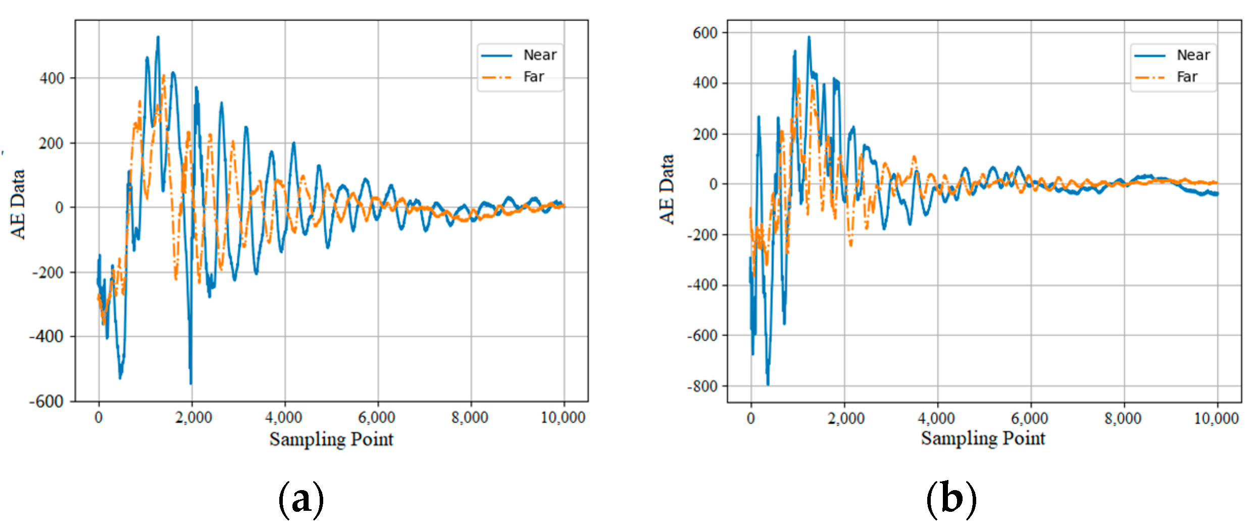
Figure 5 shows and compares the proximal/distal AE waveforms of a typical Metasequoia wood sample with different moisture contents. It is obvious that the differential terms at both ends are also largely influenced by the moisture content, and given the anisotropy of the wood, the differential values of the proximal/distal AE signal parameters can also be added to the sample data set as independent feature quantities.

2.4. Framework of WASN Moisture Content Diagnosis Method

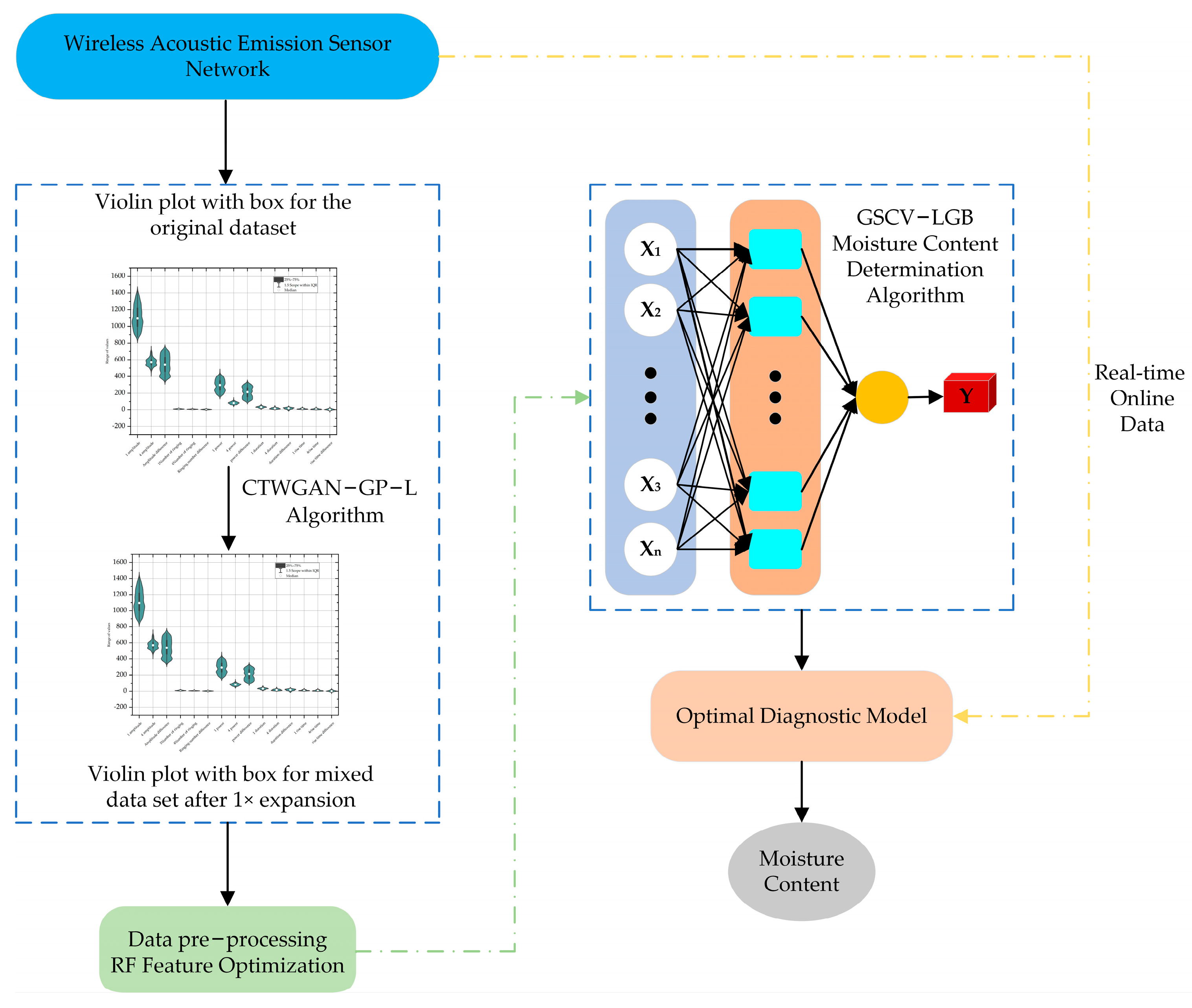
Due to the complicated sample preparation process and data collation stage, WASN is particularly susceptible to environmental factors such as temperature, humidity, and wind speed during data collection, so only a small number of feature parameters were collected as the initial sample set in this experiment, and then the proposed CTWGAN-GP-L algorithm was used to amplify the small number of feature parameters collected; finally, the original sample set and the amplified sample set were used as the sample set for the final experiment. Figure 6 illustrates the overall structure of the method for designing the moisture content diagnosis of living trees in this paper. The main idea is to use the Random Forests (RF) algorithm for feature selection of the mixed AE feature dataset, and preferably select the AE signal features with the greatest correlation with the wood moisture content as a training input to achieve the maximum expression of the original data information; then, the offline diagnostic model is established by LightGBM, and the GSCV method is used for parameter optimization to further improve the generalization ability of the model and improve the overfitting problem; finally, it is applied to the online instance prediction, and the parameter augmentation is applied to the online instance prediction. Finally, it is applied to online instance prediction, and the effectiveness of this paper’s method is verified by comparing multiple intelligent recognition algorithms.
The offline expansion of the dataset in the framework is performed in the server, while the online identification is performed on different species of trees by the WASN sensor system: first, the mixed sample dataset is pre-processed and normalized dimensionless by the CTWGAN-GP-L algorithm after a 1× expansion; then the most representative seven feature vectors are filtered based on the moisture content data labels of the prepared samples; the optimal diagnostic model is then trained using the GSCV-LGB algorithm; finally, the AE signal data collected in real time are input to the diagnostic model in order to adapt it to calculate its current moisture content value.

2.5. Generative Adversarial Networks

In recent years, generative adversarial networks (GANs) have gained great success in the field of computer vision and natural language processing, and it is one of the most creative deep learning models proposed by Ian Goodfellow et al. in 2014 [15]; however, there are relatively few studies that use GANs to expand small sample datasets to improve the diagnostic accuracy of the model.
The basic structure of the GAN model is shown in Figure 7: it consists of two main parts: the generator (G) network and the discriminator (D) network. The input of Generator G is a random noise z collected from some probability distribution (e.g., Gaussian distribution), and z is transformed by the G network (complex nonlinear transformation) to obtain the generated data Xfake.
When the input signal of the discriminator is the generated signal, the discriminator outputs the discriminant probability as close to 0 (discriminate as false) as possible. When the discriminator input signal is a generated signal, the discriminator output discriminant probability is as close to 0 (discriminate as false) as possible, while the generator generates high-quality samples with a distribution as similar as possible to make the discriminant probability close to 1 (discriminate as true). When the generator and discriminator are trained and perform well enough, i.e., when the data generated by the generator has the same distribution as the real AE feature data, the discriminator cannot distinguish whether the input data is the real AE feature data or the generated data, i.e., it is considered to reach the Nash equilibrium point in game theory [15].
The generator G and the discriminator D confront each other and represent the loss unction by V(D,G), where the discriminator seeks to minimize the error and the generator seeks to maximize the error. The training objective of the final loss function is shown in Equation (1).
min G   max D   V ( D , G ) = E x p r log D ( x ) + E z p z log ( 1 D ( G ( z ) ) )
Note: x is the real sample, G(z) is the generator-generated sample, Pr is the distribution of the real data, and Pz is the distribution of the generated data.
In actual training, the original GAN model has the problems of high training difficulty, the loss of generator and discriminator being unable to indicate the training process, and insufficient diversity of the generated samples, so CGAN (conditional generative adversarial networks) is proposed to solve the above problems well. The objective function of CGAN is shown in Equation (2).
min G   max D   V ( D , G ) = E x p r log D ( x y ) + E z p z log ( 1 D ( G ( z y ) ) )
Note: y can be auxiliary information such as class labels and the rest of the parameter information is interpreted as in the original GAN.
However, CGAN suffers from pattern collapse and gradient disappearance problems, so to improve the performance of the GAN model, many of its enhancements have been proposed in subsequent studies, including WGAN (Wasserstein GAN) [16], where Wasserstein is the bulldozer distance, and an important condition in its theory is the need to satisfy the 1 Lipschitz condition [16], whose corresponding method used is weight clipping (weight clipping). The subsequent upgraded version of WGAN also appeared, namely, WGAN-GP [17], where GP stands for the gradient penalty, which came to replace the weight clipping used in WGAN and is indeed more stable than the original WGAN from experimental results. The bulldozer distance is defined as shown in Equation (3).
W ( P r , P g ) = i n f γ Π ( P r , P g ) E ( x , y ) γ x y
Note: Π(Pr, Pg) is the set of all possible joint distributions γ ( x , y ) of the combined Pr and Pg distributions.
Subsequent studies found that WGAN still suffers from gradient explosion and gradient disappearance, so its improved version, WGAN-GP, is proposed to solve the above problems. Its objective function is shown in Equation (4).
min G   max D V ( D , G ) = E x ~ p r [ D ( x ) ] E x ˜ ~ p g [ D ( x ˜ ) ] λ   E x ^ ~ p x ^ ( ( x ^ D ( x ^ ) 2 1 ) 2 )
Note: λ is used as the gradient penalty term weight and is often taken as 10; furthermore, x ˜ is G ( z ) , and the linear interpolation between the measured AE feature parameters and the generator-generated data can be expressed by Equation (5):
x ^ = t x + ( 1 t ) x ˜ , t [ 0 , 1 ]
From what we know in deep learning, L1 and L2 regularization can solve the model overfitting problem well, so in this thesis, I innovatively add the L1 and L2 regularization expressions to obtain the mathematical equation of L regularization as shown in Equation (6).
L = λ 1 L L 1 + λ 2 L L 2 = λ 1 E x ^ ~ p x ^ x x ˜ 1 + λ 2 E x ^ ~ p x ^ x x ˜ 2 2
Note: λ 1 and λ 2 are the coefficients in front of the L1 and L2 regularization, respectively.
Finally, the objective function of the proposed CTWGAN-GP-L algorithm after the combination of CGAN, WGAN-GP and L regularization is shown in Equation (7).
min G   max D V ( D , G ) = E x ~ p r [ D ( x y ) ] E x ˜ ~ p g [ D ( x ˜ y ) ] λ E x ^ ~ p x ^ ( ( x ^ D ( x ^ y ) 2 1 ) 2 ) + L
What is more, the training objective function equations of the generator and discriminator are shown in Equations (8) and (9), respectively.
V ( G ) = E x ˜ ~ p g ( D ( x ˜ y ) )
V ( D ) = E x ~ p r [ D ( x y ) ] + E x ˜ ~ p g [ D ( x ˜ y ) ] + λ E x ^ ~ p x ^ ( ( x ^ D ( x ^ y ) 2 1 ) 2 ) + L
The corresponding pseudocode of the CTWGAN-GP-L model algorithm (Algorithm 1) can be expressed as follows:
Algorithm 1: Proposed CTWGAN-GP-L
Input: Table training dataset Ttrain, the parameter penalty coefficient λ = 10, the number of discriminator iterations per generator iteration ndiscriminator = 4, the batch size m = 8, the number of training iterations epoch = 50000. Adam hyperparameters α = 0.0001, β1 = 0, β2 = 0.9. The initial discriminator parameter is w0, and the initial generator parameter is θ0.
Output: Generate false AE feature data.
1:While θ has not yet converged do
2:     for t = 0, …, ndiscriminator do;
3:        for i = 1, …, m do;
4:          Sample the real data x ~ Pr,y conditions, the implicit variable z ~ p(z), and a random number t ~ U [0, 1].
5:                     x ˜ G θ ( z y ) ;
6:          Calculate the linear interpolation x ^ by Equation(5);
7:          Calculate L by Equation(6);
8:                     V ( D ) D w ( x y ) + D w ( x ˜ y ) + λ ( ( x ^ D ( x ^ y ) 2 1 ) 2 ) + L ;
9:       end for
10:             w A d a m ( w V ( D ) , w ,   α ,   β 1 ,   β 2 ) ;
11:   end for
12:   sample a batch of latent variables { z ( i ) } i = 1 m ~ p ( z ) .
13:       V ( G ) D w ( x ˜ y ) ;
14:       θ A d a m ( θ V ( G ) , θ , α , β 1 ,   β 2 ) ;
15: end while
CTGAN algorithm model was proposed by Lei Xu et al. in 2019 [18]. Before this algorithm was proposed, Lei Xu et al. also proposed the Tabular GAN (TGAN) algorithm model [19], but the quality of the generated data was not high in this algorithm model due to the lack of conditions as a guide to generate the data; however, in CTGAN normalization for patterns was invented to overcome the non-Gaussian and multi-modal distributions. The difference between the CTGAN and normal Generative Adversarial Network (GAN) network structure is shown in Figure 8.

2.5.1. GAN Model Generates Data Quality Assessment Metrics

Assessing the quality of the data generated by GAN models is very difficult and finding the appropriate assessment metrics is even more difficult. In the literature [20], a comparative analysis of several common GAN quantitative evaluation metrics was conducted, and the results showed that two evaluation metrics, maximum mean difference (MMD) and 1-nearest neighbor (1-NN), are excellent for identifying mode collapsing and mode missing and detecting overfitting, so in this paper, MMD and 1-NN are preferred for evaluating the generated AE feature parameters. In this paper, MMD and 1-NN are preferred for the evaluation metrics of the generated AE feature parameters.
The kernel MMD is defined as shown in Equation (10).
M M D 2 ( P r , P g ) = E x r , x r p r x g , x g p g [ k ( x r , x r ) 2 k ( x r , x g ) + k ( x g , x g ) ]
Note: x r and x r represent two samples obtained by sampling from the real data distribution, x g and x g represent two samples obtained by sampling from the generated data distribution.
MMD is a measure of the difference between two distributions in Hebert space, so the distance between the original input AE feature parameter dataset Pr and the generated dataset Pg can be considered using the MMD measure, and then, this distance is used as an evaluation metric for the CTWGAN-GP-L algorithm. If the MMD distance is smaller, it indicates that the quality of the generated AE feature parameters is better.
1-NN is the n samples x1, …, xn of the AE feature parameter dataset Pr from the original input and the n samples y1, …, yn from the generated dataset Pg. Calculate the accuracy of LOO (leave-one-out) using 1-NN, and use the accuracy as an evaluation metric for the CTWGAN-GP-L algorithm. Special attention is paid to the fact that the closer the LOO is to 50%, the more the AE feature parameters generated by the generator meet the requirements, i.e., the ideal value of the 1-NN metric is 0.5, and the lower the value is between 0.5 and 1, but if it is lower than 0.5, the generated data are overfitted.

2.5.2. CTWGAN-GP-L Algorithm Construction

Because the proposed CTWGAN-GP-L algorithm shows strong advantages in data generation, it is chosen for data enhancement in this paper. Both the generator and the discriminator use fully connected networks, and 900 × 15 sets of AE feature parameters are selected for training the CTWGAN-GP-L algorithm model. In the training process, the generator receives Gaussian noise data to generate AE feature parameters with a similar distribution to the real data, called fake data; then, the fake data and the real data are used as the input of the discriminator, which tries to distinguish the fake data from the real data.
Finally, the objective functions of the generator and the discriminator are built according to Equations (8) and (9), respectively, for adversarial training. The network parameters of the generator and discriminator in the proposed CTWGAN-GP-L algorithm model are shown in Table 1 and Table 2, respectively.

2.5.3. Synthetic Minority Oversampling Technique (SMOTE) Algorithm

The Synthetic Minority Oversampling Technique (SMOTE) algorithm is an oversampling algorithm that synthesizes a small number of class samples [21], which is an improved scheme based on the random oversampling algorithm. It is well known that if the number of each class in a certain dataset is inconsistent, especially the kind that shows extreme data imbalance, this can seriously affect the classifier accuracy, and sometimes misclassification may occur because the minority class will be masked by the majority class. However, this paper applies the SMOTE algorithm for the first time to data augmentation on balanced datasets for a comparative analysis of other data expansion methods.

2.5.4. Datasets

In the experimental process, in order to verify whether the proposed CTWGAN-GP-L algorithm model, can successfully learn to generate real data, so two datasets were first selected from the University of California, Irvine (UCI) data repository for testing. The first dataset is the Abalone dataset with the first column of attributes, which are all English characters, representing the sex of abalone, M for male, F for female, and I for juvenile, and the English characters “M, F, I” are used as numbers “0, 1, 2”, respectively, for the classification task. To be suitable for the classification task, the English characters “M, F, I” are replaced by the numbers “0, 1, 2”, respectively, and the rest of the columns remain unchanged as attribute columns, as shown in Table 3.
From Table 3, we can see that the Abalone dataset has a category imbalance problem, and the few categories provide less information than the majority categories, so the model does not get enough information to ignore the few categories, and sometimes misclassification occurs, and the number of samples in each category is too small, which also leads to a decrease in classification accuracy. Therefore, the data set is first reduced to a balanced data set, i.e., the number in each category becomes 1300.
The second dataset is the image segmentation dataset. The first column of this dataset is the attribute column, and all of them are English characters, where BRICKFACE stands for face brick, SKY stands for sky, FOLIAGE stands for leaf, CEMENT stands for cement, WINDOW stands for window, PATH stands for road, and GRASS stands for grass. In order to apply to the classification task, the seven categories are replaced by the numbers “1~7”, respectively, and the rest of the columns remain unchanged as attribute columns, as shown in Table 4.
From Table 4, we can see that the number of data in each category in the Image Segmentation dataset is 330, so there is no need to balance it again. Finally, the CTWGAN-GP-L algorithm model was used again to expand the data for the abalone dataset, the Image Segmentation dataset and the 900 × 15 groups of AE feature parameters collected by our own experiments, respectively, to further demonstrate that the proposed algorithm model can improve the classification accuracy, which helps the final diagnosis of live standing wood moisture content.

2.5.5. Model Training

Since the CTWGAN-GP-L algorithm model training needs some real data, the original data set is first expanded by 1×, 2× and 3×, and then the expanded 1×, 2× and 3× data are added to the original data set to verify the highest classification accuracy when the ratio of the final generated data to the original data. The loss values of the generator and discriminator are shown in Figure 9, which shows that the generator and discriminator converge to 0 after a certain number of rounds of training, indicating that the training is gradually optimized to the best state.
The experimental environment in this experiment is shown in Table 5.

2.5.6. Generating Data Quality Assessment

In order to verify the quality of the data generated by the CTWGAN-GP-L algorithm model, this section utilizes the evaluation metrics MMD and 1-NN proposed in Section 2.5.1 to evaluate the quality of the generated data. Table 6 shows the quality of the generated 1-fold data of the four algorithm models SMOTE, TGAN, CTGAN, and CTWGAN-GP-L using the two metrics MMD, 1-NN on the Abalone dataset, Image Segmentation dataset and 900 × 15 group AE feature parameter dataset, respectively.
From Table 6, it can be seen that the CTWGAN-GP-L algorithmic model proposed in this paper outperforms the remaining three algorithmic models in terms of data generation quality under all three datasets, which leads to the conclusion that the CTWGAN-GP-L algorithmic model is feasible for tabular data generation and that the values obtained for the MMD and 1-NN evaluation metrics under all four algorithmic models are within the acceptable range.
In addition to this, Justin Engelmann et al. compared univariate distribution plots (kernel density estimation plots) and count plots of the true and generated distributions of the numerical and categorical columns of the UCI adult dataset [22]. Let the probability density function of kernel density estimation be f. For one-dimensional data with sample size n, the mathematical expression of the probability density function derived using kernel density estimation at point x is shown in Equation (11).
f ( x , h ) = 1 n i = 1 n K h ( x x i ) = 1 n h i = 1 n K ( x x i h )
Note: K is the kernel function and h is the bandwidth.
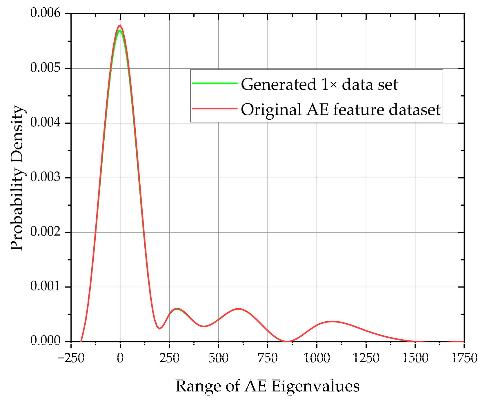
To further evaluate the quality of the data generated by the CTWGAN-GP-L algorithm model, we first plotted the hybrid kernel density estimates for the numerical columns of the original AE feature parameter dataset and the generated 1-fold dataset, which are shown in Figure 10.
The kernel density curves of the two datasets match very well, which indicates that the data distributions are very similar and the quality of the generated data is also high from the side. This graph is a variant of the histogram that uses a smoothing curve to plot the horizontal values, resulting in a smoother distribution. Kernel density estimation charts are superior to histograms in that they are not affected by the number of groupings used, so they can better define the shape of the distribution.
Vision is a very powerful tool in human verification of results and pattern recognition, so visual evaluation plays a crucial role in the evaluation process of the model. Stavroula Bourou et al. used one discrete feature and two continuous features to perform a plot analysis of the cumulative sum of the original and synthetic data [23], but they only examined the distribution between the columns for a particular column or columns of similarity. In this paper, I innovatively integrate the 15 columns of AE features in the 1× data generated by the CTWGAN-GP-L algorithm and the 15 columns of AE features in the original data by normalizing them separately in a single plot for overall accumulation and analysis, where the statistics of the real data are marked in blue and the statistics of the synthetic data are marked in orange, and the displayed results are shown in Figure 11.
It can be seen from Figure 11 that the cumulative and distribution of the generated data and the columns of the original data after integration are very similar, indicating that the proposed CTWGAN-GP-L algorithm works very well in this piece of table data generation.

2.6. Diagnostic Accuracy Assessment of Living Tree Moisture Content

The results obtained from the multiple data generation evaluation metrics in Section 2.5.6 show that the proposed CTWGAN-GP-L algorithm model can generate high-quality data, but the ultimate goal of data set expansion is to improve the diagnostic accuracy of standing wood moisture content, so it is still necessary to verify how much data is generated to add to the original data set with the highest classification accuracy. So, the next set of experiments was designed to expand the original AE feature dataset to 1×, 2×, and 3× using the CTWGAN-GP-L algorithm model, respectively, and then calculate the corresponding classification accuracy using the unoptimized LightGBM classification algorithm, respectively.
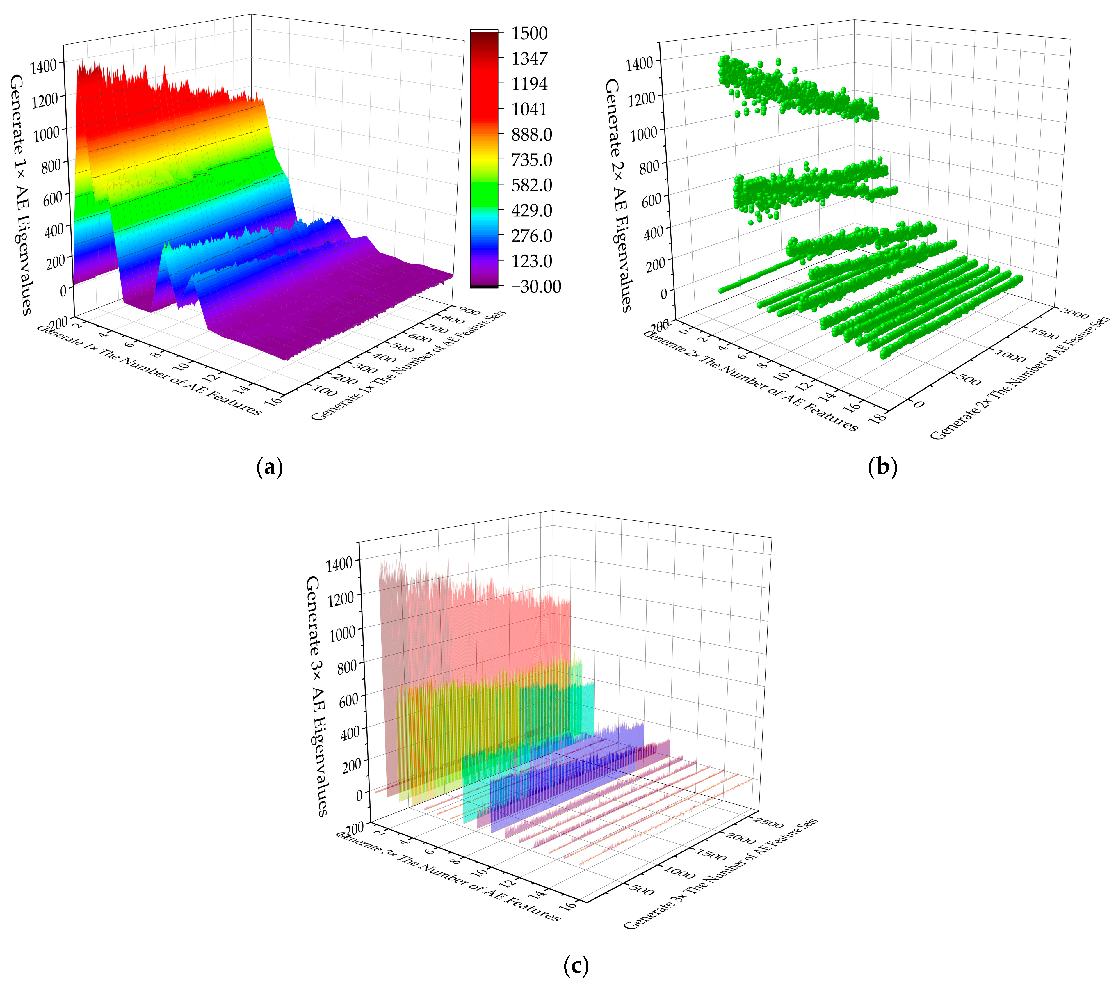
Figure 12 shows the 3D data maps generated by expanding the AE feature dataset by 1×, 2×, and 3× using the CTWGAN-GP-L algorithm, followed by the classification measured accuracy of the original dataset and its blending with the original dataset by 1×, 2×, and 3×, respectively, as shown in Figure 13.
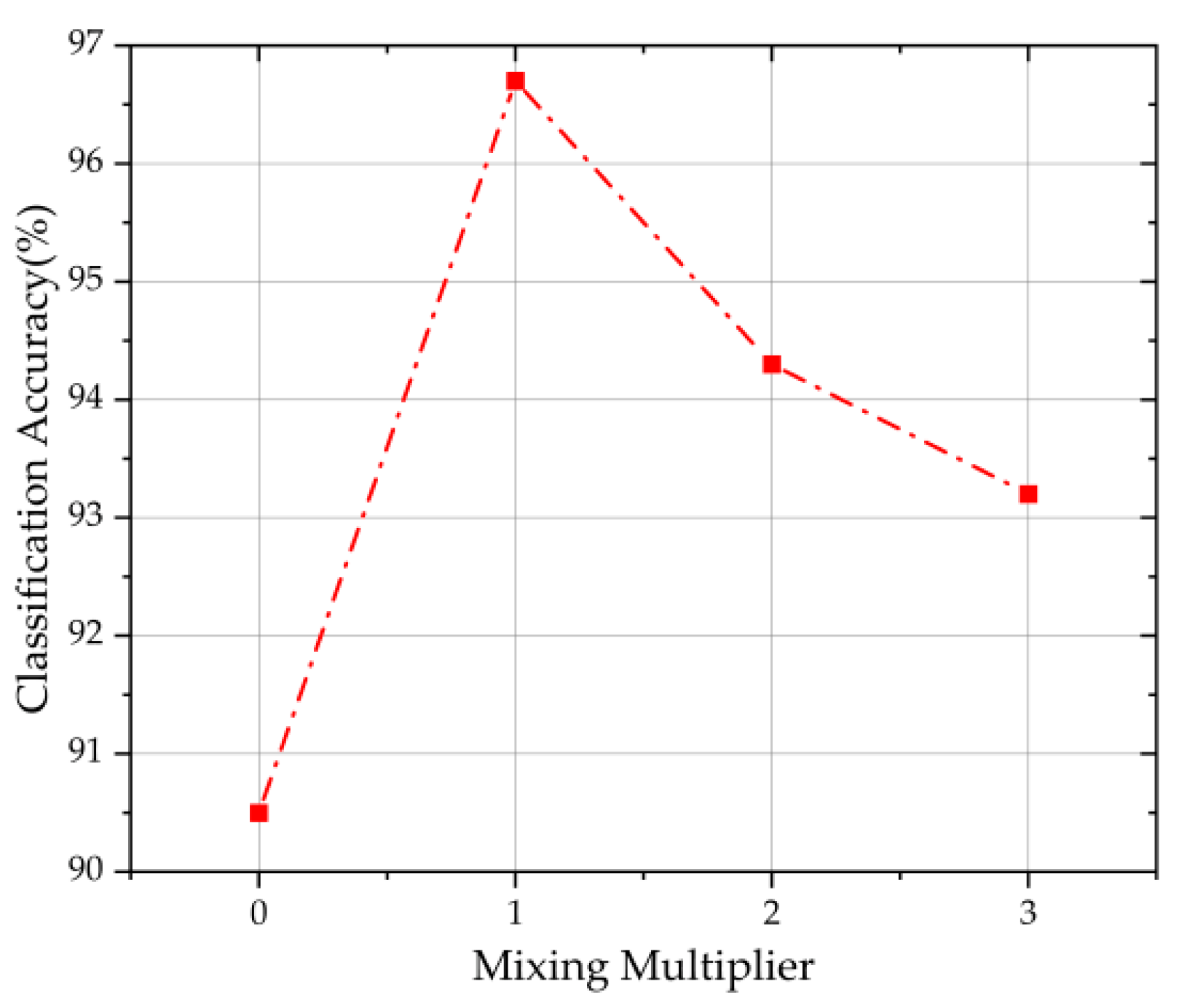
From Figure 13, we can see that the classification accuracy of the original dataset is only 90.5%, and the highest accuracy is 96.7% when the dataset is expanded to a multiple of 1. After that, the classification accuracy decreases gradually with the increase in the multiple, but it is still more classification accurate than the dataset without expansion. Therefore, it is meaningful to use the CTWGAN-GP-L algorithm to expand the dataset, and when the amount of data measured by us is limited, expanding the original dataset to a certain number of times can achieve the purpose of improving the accuracy of moisture content diagnosis.

2.7. Random Forest (RF) Algorithm

The common feature selection methods are Filter, Wrapper, and Embedded, and the integration method is generated by combining the Filter and Wrapper methods. In this paper, the random forest algorithm [24], which is one of the integration methods, is chosen to compare and analyze the feature importance ranking in the feature selection process with the XGBoost algorithm.

2.8. Light Gradient Boosting Machine (LightGBM) Algorithm

The Light Gradient Boosting Machine (LightGBM) algorithm was proposed by Ke G et al. in 2017 [25]. Numerous experiments have shown that it outperforms GBDT, eXtreme Gradient Boosting (XGBoost), and traditional machine learning methods in terms of performance, efficiency, and running speed, and the LightGBM algorithm is optimized for traditional gradient boosting trees using two algorithms: one-sided gradient sampling and mutually exclusive feature binding.

2.9. Design of WASN Moisture Content Diagnosis Method

2.9.1. Acquisition Data and Feature Selection

Samples were prepared according to the international standard GB/T 1931-2009 (the selected species was Metasequoia, 37.5 cm high, 9 cm diameter near cylinder), and their corresponding moisture content values were 10%, 15%, 20%, 25%, 30%, 35%, 40%, 45%, 50% (error ± 1%), and the physical diagrams of sample data collection and calibration diagrams of moisture content data are shown in Figure 14 and Figure 15, respectively.
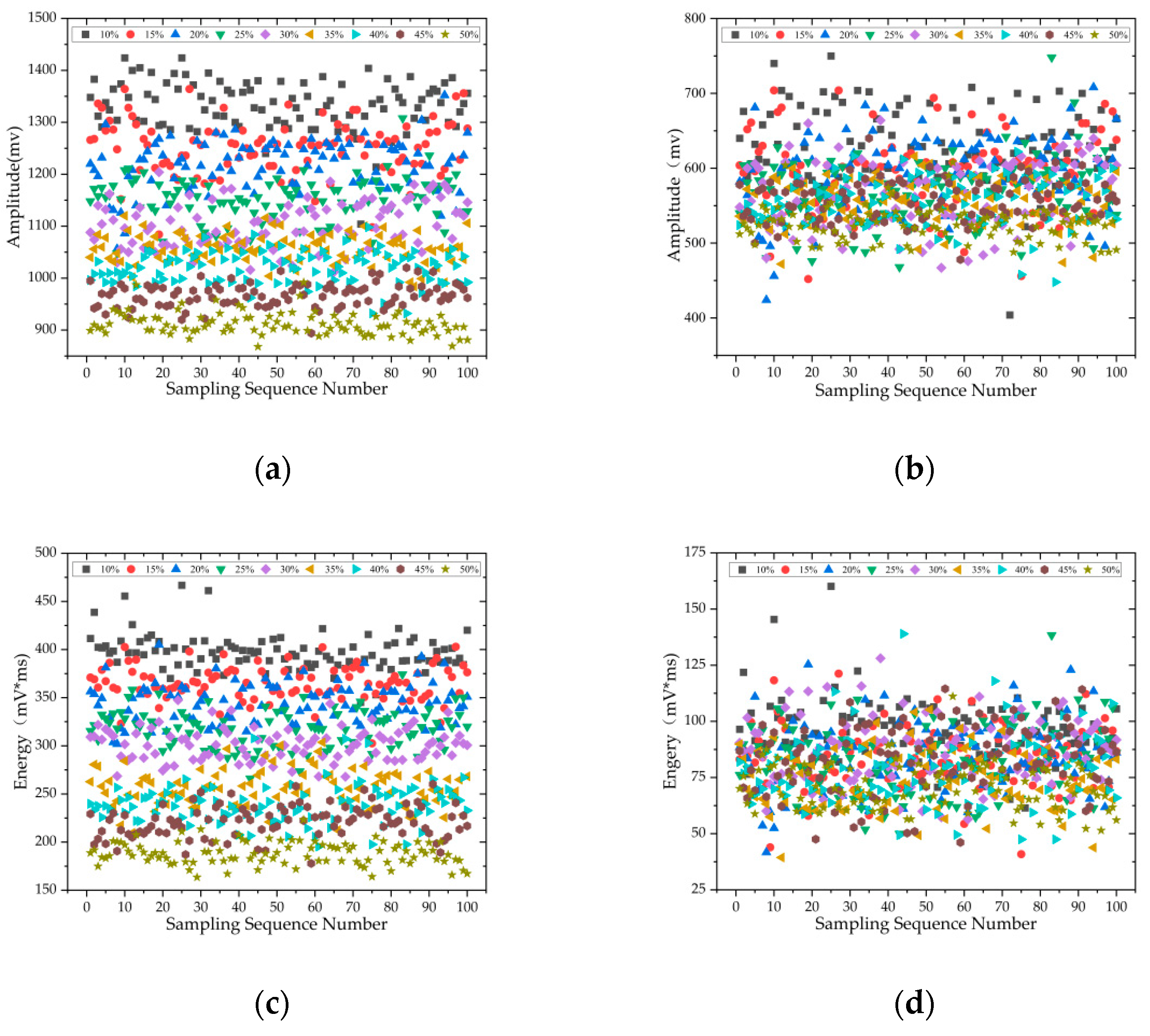
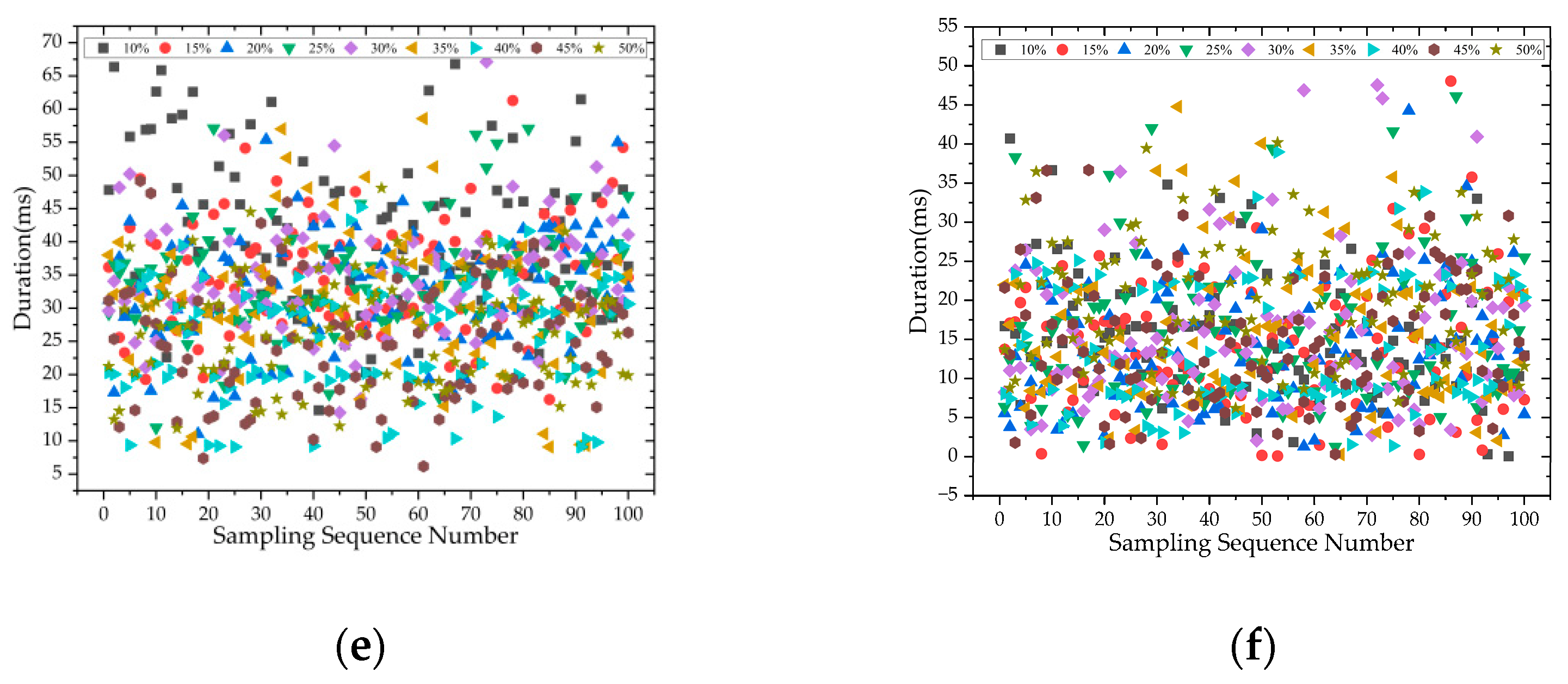
The wood is coupled to the AE sensor via petroleum jelly for enhanced signal transfer. The nodes were sampled 100 times for each of the 9 samples, and each set of data then contained the following characteristics of the proximal/distal AE signal: amplitude, rise time, duration, ringing count, energy, and the differential value of the proximal/distal parameters, for a total of 15 parameters. Some of the results are shown in Figure 16 below.
Next, the mixed data set consisting of the original AE data and the generated 1× data is normalized to between 0 and 1.
x i = x i x min x max x min ; i = 1 , 2 ,
xmin and xmax are the minimum and maximum values of the input mixed feature data, respectively, and xi* and xi are the normalized data and mixed data, respectively. Then, the data matrix of AE parameter feature set (1800 × 15) is constructed and used as the input of RF, while the corresponding moisture content (10%, 15%, 20%, 25%, 30%, 35%, 40%, 45%, and 50%) constitutes the label vector.
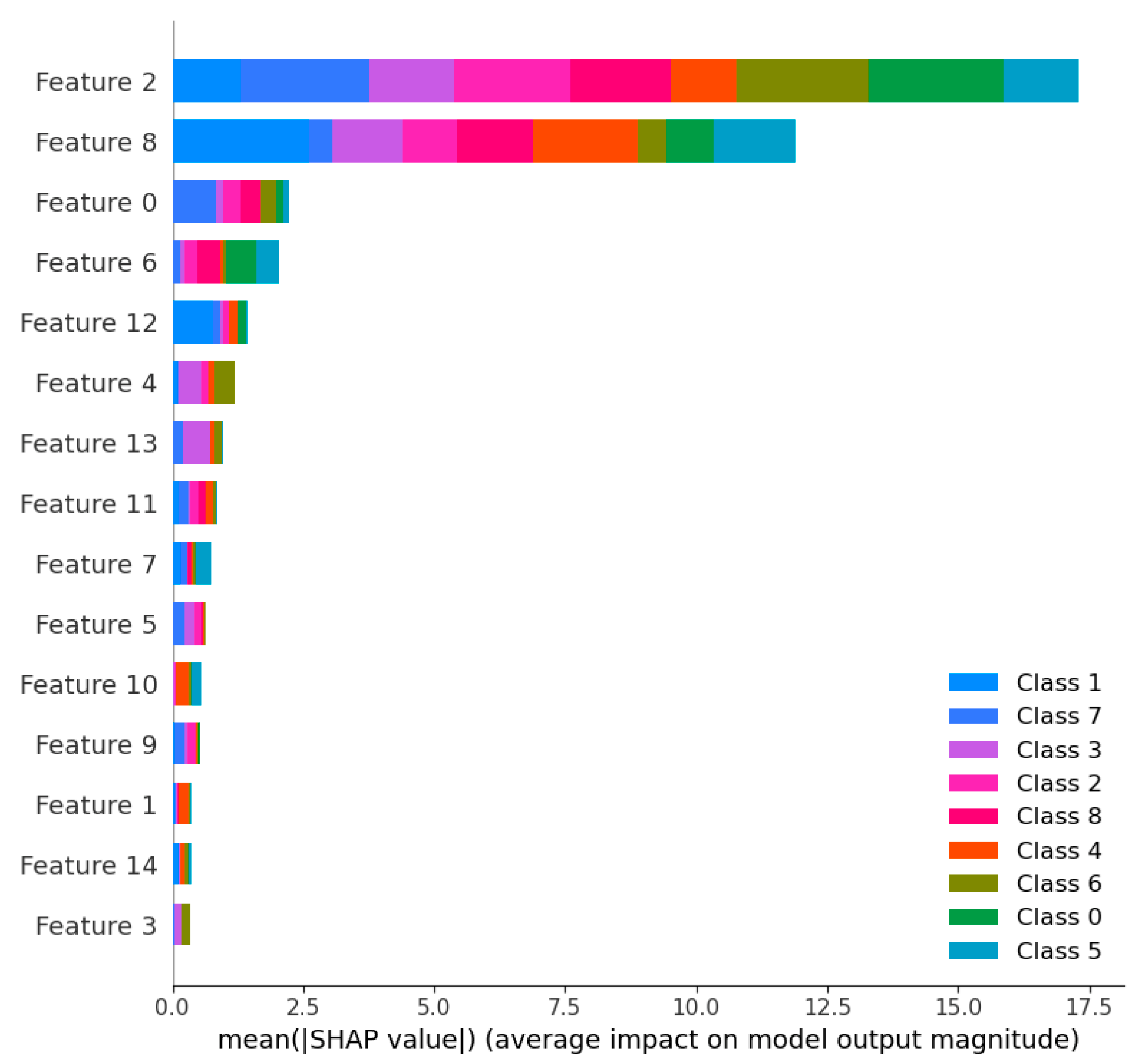
One of the ways to calculate feature importance in the RF algorithm is to use SHAP (SHapley Additive exPlanation), which is an explanatory model of additivity constructed by Lundberg et al. inspired by cooperative game theory [26]. Assuming that the number of the most optimal feature set is 15, the results of the superiority ranking of all AE feature quantities are shown in Figure 17.
The graph of the results of the screening features by the RF algorithm can be organized in the order shown in Table 7.
Finally, the number of the best feature set is incremented from 1, and LightGBM with default parameter configuration is used for training and testing, and the box line plot corresponding to the recognition accuracy can be obtained as shown in Figure 18. However, when the number of features is 10, the accuracy rate increases, but it is still lower than that when the top 7 features are used to build the feature subset. Therefore, this paper uses the top 7 features for the analysis of the moisture content diagnosis algorithm.

2.9.2. GSCV-LGB Diagnostic Algorithm

The grid search and cross-validation (GSCV) algorithm searches for parameters, i.e., adjusts the parameters in order by step within the specified parameter range, trains the learner with the adjusted parameters, and finds the parameter with the highest accuracy in the validation set from all the parameters, which is actually a training and comparison process. The k-fold cross-validation divides the entire data set into k copies and uses the remaining k-1 copies as the training set to train the model. The k-fold cross-validation divides the entire data set into k copies, and each copy is used as the test set without repetition, and the remaining k-1 copies are used as the training set for training the model. Based on this, the GridSearchCV algorithm is applied to the parameter search of LightGBM, and the optimal hyperparameters are selected to establish the GSCV-LGB diagnosis model with the highest recognition accuracy of LightGBM as the optimization goal.

3. Results

3.1. Experiment and Analysis of Standing Wood Moisture Content Measurement System

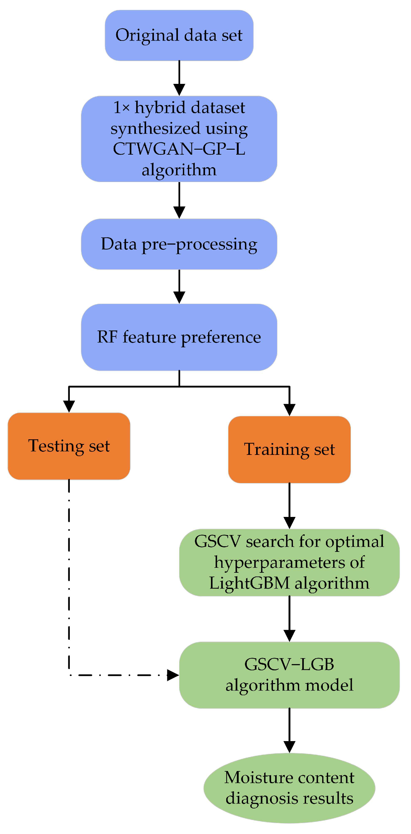
Figure 19 shows the optimization of the LightGBM hyperparameters by the GridSearchCV algorithm and the process of building a moisture content diagnostic model using the optimized GSCV-LGB algorithm. After the aforementioned feature selection and sample set determination, the optimal hyperparameters of the LightGBM algorithm can be found within the specified parameter range; the optimal hyperparameters are then substituted back into the LightGBM algorithm, and finally, the GSCV-LGB moisture content diagnostic model is obtained for real measurement.

3.2. Algorithm Validation

A total of 900 sets of offline data samples were collected from the actual measurement of Metasequoia samples by WASN, including 100 sets of each of 10%, 15%, 20%, 25%, 30%, 35%, 40%, 45%, and 50% moisture content samples, which were then expanded by the CTWGAN-GP-L algorithm by a factor of 1 and then randomly divided into two in the ratio of 8:2, i.e., 1440 sets of training samples and 360 groups of test samples. In order to verify the effectiveness of the RF feature selection algorithm and the superiority of the GSCV-LGB moisture content recognition algorithm, two sets of experiments were designed in this paper: the first set of experiments compared the moisture content recognition results of the features screened by the XGBoost method and the RF selected features, in which the recognition algorithm uniformly used the LightGBM with default parameters; in the second set of experiments, the results of the Decision Tree (DT) algorithm, the DT algorithm optimized by GridSearchCV, the RF algorithm, the RF algorithm optimized by GridSearchCV, the LightGBM algorithm, and the LightGBM algorithm optimized by GridSearchCV were compared for the identification of the target moisture content, and here the results used for the feature vectors for training are uniformly constructed from the results filtered by the RF algorithm. In both groups, the accuracy, weighted avg, precision, recall, F1-score, MCC, and ROC-AUC are used as evaluation metrics.
The accuracy rate is the proportion of correctly classified samples to the total tested samples, as shown in Equation (13).
A c c u r a c y = T P + T N T P + T N + F P + F N
The weighted average is the weighted average of each category of assessment indicators, as shown in Equation (14).
W e i g h t e d   a v g = ( i = 1 n p r e c i s i o n i / r e c a l l i / f 1 - s c o r e i ) × s u p p o r t i i = 1 n s u p p o r t i
Note:/means or and support means the number of correctly classified samples in each class label.
Precision is the probability that all samples classified as correct are actually correct, as shown in Equation (15).
P r e c i s i o n = T P T P + F P
Recall is the probability of being classified as the correct sample out of the actual correct sample, as shown in Equation (16).
R e c a l l = T P T P + F N
The F1-score is the summed average of precision and recall, as shown in Equation (17).
F 1 - s c o r e = 2 × P r e c i s i o n × R e c a l l P r e c i s i o n + R e c a l l
The Mathews correlation coefficient (MCC) is the correlation coefficient between the actual classification and the predicted classification, which takes values in the range of −1 to 1, as shown in Equation (18).
M C C = T P × T N F P × F N ( T P + F P ) ( T P + F N ) ( T N + F P ) ( T N + F N )
TP, FP, TN, and FN involved in Equations (13)–(18) denote true positive, false positive, true negative, and false negative, respectively.

3.3. Feature Selection Performance Analysis

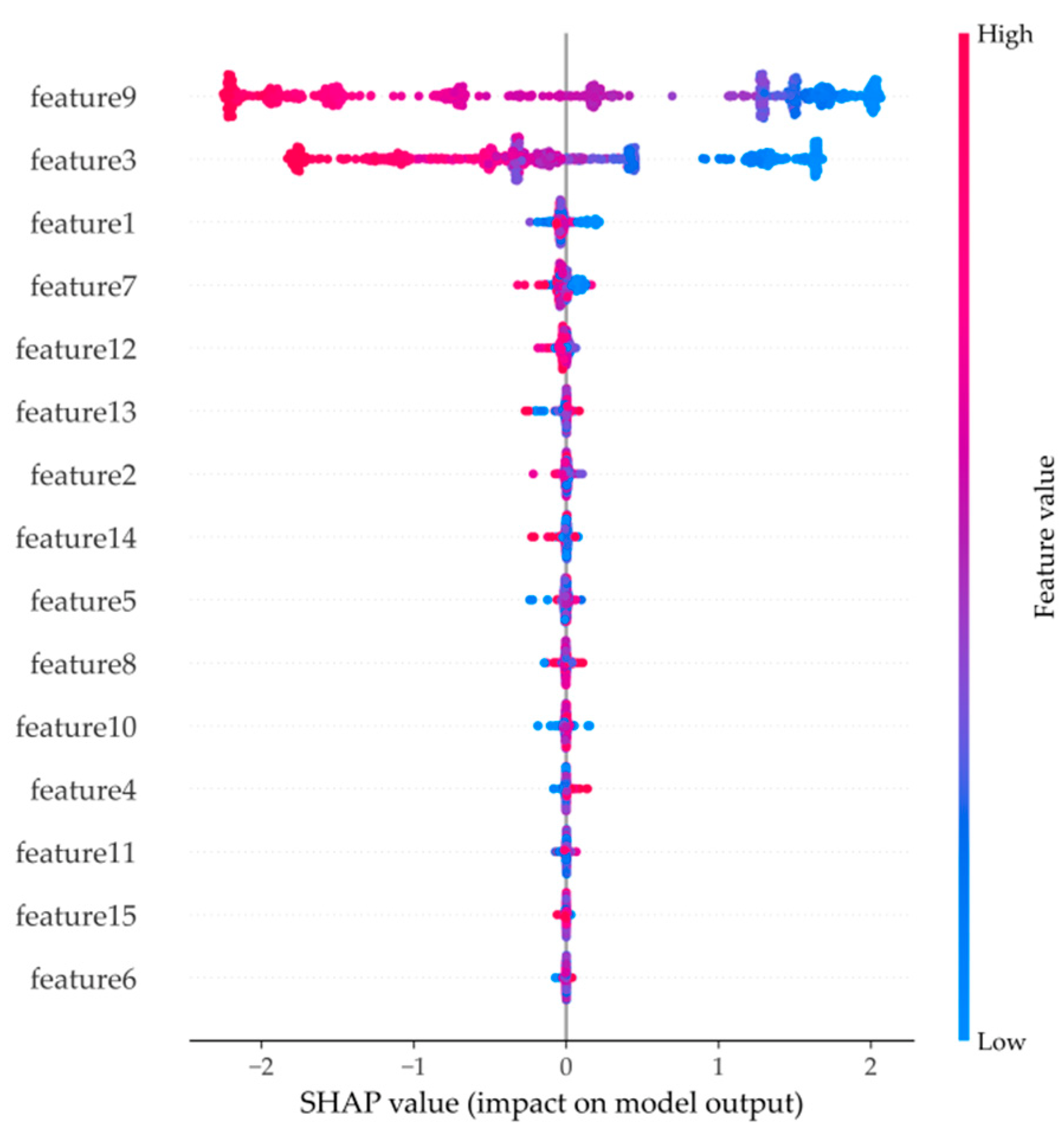
Again, using Shap to explain the final feature selection ranking of the XGBoost algorithm model is shown in Figure 20, where the vertical coordinates indicate the feature variables from top to bottom as proximal/distal amplitude difference, proximal/distal energy difference, proximal amplitude, proximal energy, proximal rise time, distal ringing count, distal rise time, proximal/distal duration difference, distal energy, proximal/distal ringing count difference, proximal/distal energy difference, proximal duration, distal amplitude, proximal/distal rise time difference, and proximal ringing count.
It is obvious from the figure that the top 11 features have a larger proportion, so four features, such as proximal duration, distal amplitude, proximal/distal rise time difference, and proximal ringing count, can be deleted.
The feature screening results of the RF algorithm and the XGBoost algorithm are next presented in Table 8. From Table 8, it can be seen that when using the 11-dimensional features of the XGBoost algorithm for LightGBM recognition, the accuracy is only 85.5%; while using the features screened by RF for recognition, the accuracy is increased to 96.2%. Compared with the results of XGBoost, the RF algorithm preferred features with lower dimensionality parameters and higher recognition accuracy, proving its efficiency in AE signal feature selection in WASN.

3.4. Comparison of the Effects of Different Intelligent Diagnostic Methods

In this section, six methods, DT algorithm, GSCV-DT algorithm, RF algorithm, GSCV-RF algorithm, LightGBM algorithm, and GSCV-LGB algorithm, were selected for the comparison test of moisture content diagnosis. All of them use the expanded and RF feature-preferred AE feature data set as input, and the test results are shown in Table 9.
The diagnostic results in Table 9 show that the recognition accuracy of the optimized LightGBM algorithm is higher than that of the unoptimized LightGBM algorithm, RF algorithm, and DT algorithm as well as the optimized RF algorithm and DT algorithm, where the recognition accuracy of the unoptimized LightGBM algorithm, RF algorithm, and DT algorithm are 96.2%, 93.5%, and 92.8%, respectively, and the optimized LightGBM algorithm, RF algorithm, and DT algorithm have recognition accuracies of 97.9%, 94.4%, and 93.9%, respectively. The initial values of each hyperparameter of the DT algorithm and the final hyperparameter values optimized by the GSCV algorithm are listed in Table 10. Table 11 lists the initial values of each hyperparameter of the RF algorithm and the final hyperparameter values optimized by the GSCV algorithm. Table 12 shows the initial values of the hyperparameters of the LightGBM algorithm and the final hyperparameters optimized by the GSCV algorithm.
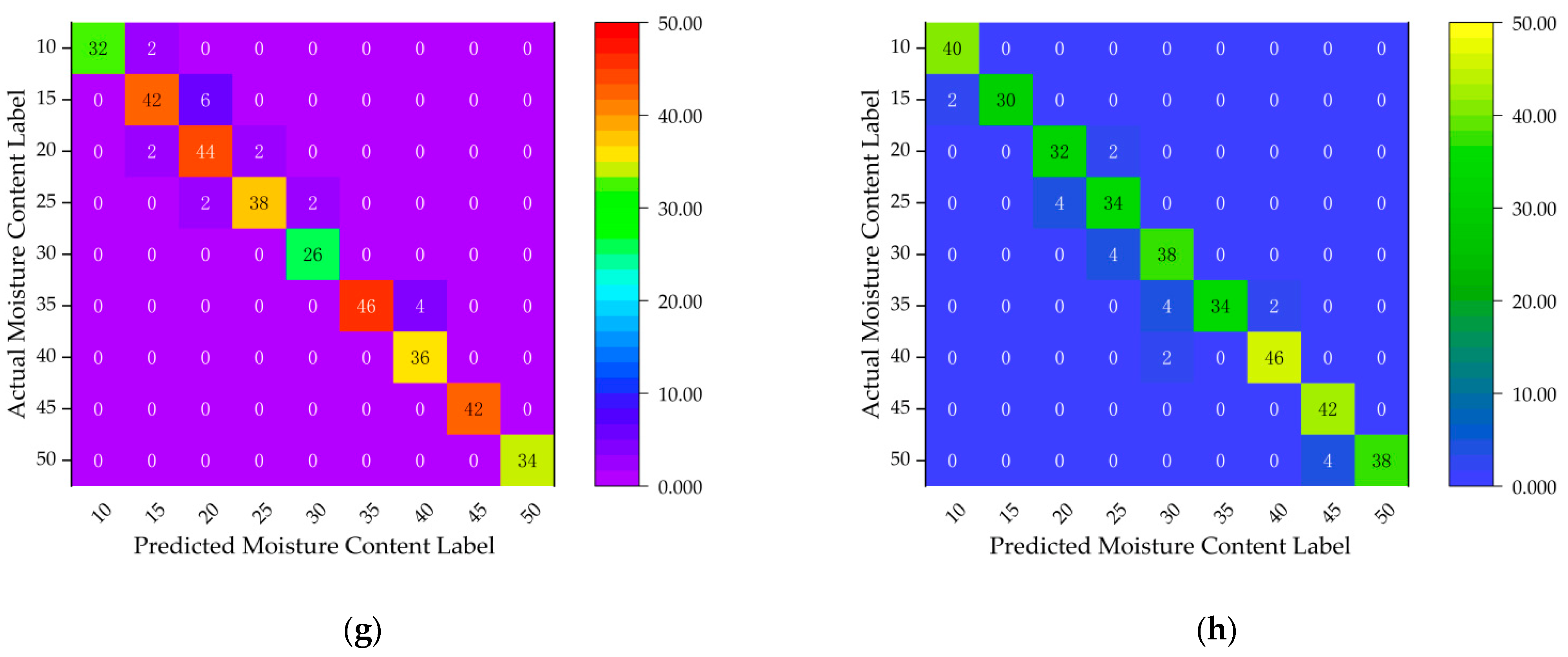
The comparison plots of each evaluation metric of the GSCV-LGB classification algorithm with the GSCV-RF classification algorithm and the GSCV-DT classification algorithm are shown in Figure 21a–h, respectively.
From Figure 21a, it can be seen that the precision of the GSCV-LGB algorithm is lower than that of the GSCV-RF algorithm at 10% and 45% of the moisture content label value, and lower than that of the GSCV-DT algorithm at 10%; in addition, the precision of the GSCV-LGB algorithm is consistent with that of the GSCV-RF algorithm and GSCV-DT algorithm at 25%, 35%, and 50% of the moisture content label value, respectively. The precision of the GSCV-LGB algorithm is higher than that of the GSCV-RF algorithm and GSCV-DT algorithm in all other cases.
From Figure 21b, we can see that the recall rate of the GSCV-LGB algorithm is lower than that of the GSCV-RF algorithm at 30% and 50% of the moisture content label value and lower than that of the GSCV-DT algorithm at 15% of the moisture content label value; in addition, it is consistent with the GSCV-RF algorithm at 40% and 45% of the moisture content label value, and it is consistent with the GSCV-DT algorithm at 45% of the moisture content label value. The recall rate of the GSCV-LGB algorithm is higher than that of the GSCV-RF algorithm and GSCV-DT algorithm in all other cases.
In addition, it can be seen from Figure 21c that the F1-score of the GSCV-LGB algorithm is lower than that of the GSCV-RF algorithm except for the 30% moisture content label value and the 10% and 15% moisture content label values, respectively, where the F1-score is lower than that of the GSCV-DT algorithm; in all other cases, the F1-score of the GSCV-LGB algorithm is higher than that of the GSCV-RF and GSCV-DT algorithms for each type of wood. The F1-score of the GSCV-LGB algorithm is higher than that of the GSCV-RF algorithm and the GSCV-DT algorithm for all other cases.
Then, it can be seen from Figure 21d that the MCC value of the GSCV-LGB algorithm is lower than that of the GSCV-RF algorithm except for the value of the moisture content label of 25%, and the value of the moisture content label of 10% is lower than that of GSCV-DT algorithm; in addition, the MCC value of moisture content label of 30% is consistent with that of the GSCV-RF algorithm and GSCV-DT algorithm. The MCC value of the GSCV-LGB algorithm is higher than that of the GSCV-RF algorithm and GSCV-DT algorithm in all other cases.
Furthermore, it can be seen from Figure 21e that the ROC curves of the GSCV-LGB algorithm are both above those of the GSCV-RF algorithm and the GSCV-DT algorithm, and the AUC values are also larger than those of the GSCV-RF algorithm and the GSCV-DT algorithm, from which it can be seen that the classification effect of the GSCV-LGB algorithm is better than that of the GSCV-RF algorithm and the GSCV-DT algorithm.
Finally, comparing plots Figure 21f–h, it can be seen that the GSCV-LGB algorithm predicts fewer correct labels than the GSCV-RF algorithm for moisture content label values of 20% and 35%, and fewer correct labels than the GSCV-DT algorithm for moisture content label values of 20% and 25%; in addition, the GSCV-LGB algorithm predicts fewer correct labels than the GSCV-RF algorithm for moisture content label values of 25% and 40%; in the remaining cases, the GSCV-LGB algorithm predicts fewer correct labels than the GSCV-RF algorithm and the GSCV-DT algorithm. In addition, the GSCV-LGB algorithm predicts the same number of correct labels as the GSCV-RF algorithm at 25% and 40% of the moisture content labels; in the rest of the cases, the GSCV-LGB algorithm predicts a higher number of correct labels than the GSCV-RF algorithm and the GSCV-DT algorithm.

4. Discussion

4.1. Analysis of Live Trees

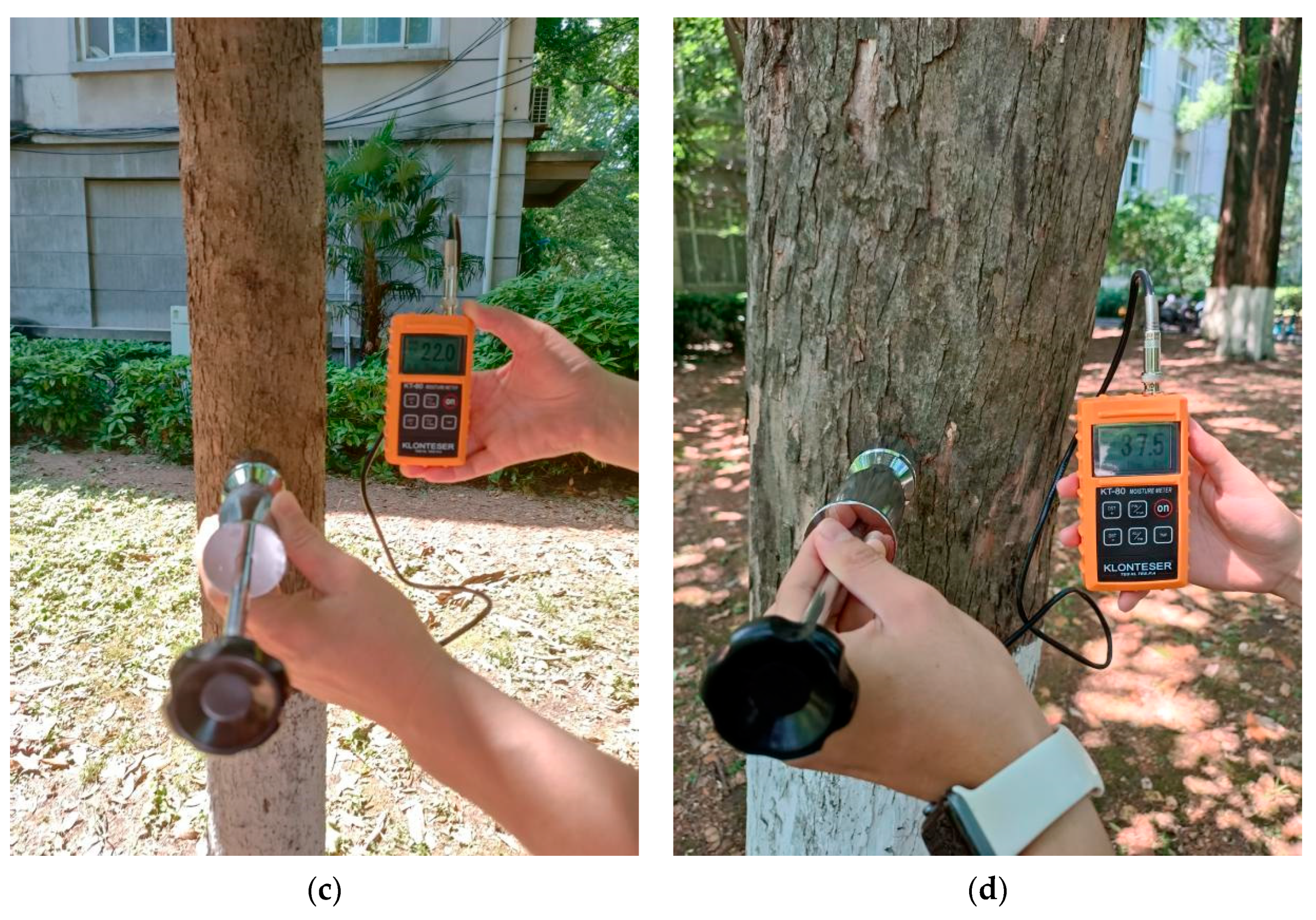
In order to verify the effectiveness of the moisture content diagnostic method designed in this paper on different standing trees, AE data were collected for analysis in field tests on standing trees such as magnolia, zelkova, triangle maple, zhejiang nan, ginkgo, and yunnan pine on the South Forest campus and then use KT-80 high-precision moisture tester imported from Italy for multi-point average calibration (measuring moisture content of 44.5%, 22.0%, 37.5%, 48.7%, 38.6%, 49.3%, respectively); the installation test and calibration plots for zhejiang nan and triangle maple are shown in Figure 22a–d, respectively.
The confusion matrix of the recognition results of six species of live standing trees is shown in Table 13. The confusion matrix is represented by an N-dimensional matrix, which is mainly used for comparison between the results obtained by model classification and the actual results measured by high-precision instruments. From Table 13, we can see that the nondestructive diagnosis method of live standing wood moisture content by the wireless acoustic emission sensor system designed in this paper has a good diagnosis ability with an accuracy rate of more than 97.4%, and the system can accurately identify the moisture content of coniferous trees, broad-leaved trees, and other trees, which proves that the diagnosis model has a strong generalization ability and good robustness.

4.2. System Energy Consumption Exploration

The power consumption of this WASN node is mainly composed of three parts: the energy consumption of micro vibration motor, the energy consumption of LoRa wireless communication, and the energy consumption of analog-to-digital converter AD7356 and preamplifier OPA627 chip, which consume 280 mW, 100 mW, and 111 mW, respectively. However, since the wireless nodes are in work/sleep mode, their work/sleep duty cycle is often set to about 3%, and the AE signal measurement is only performed three times a day (i.e., once every 8 h). Therefore, the total energy consumption of the system is about 1500 mW/day. If combined with the 3.7 V 30Ah Li-ion battery pack, the normal working life cycle of each wireless node can reach 74 days. It can basically meet the field-independent application requirements of forestry IoT.

5. Conclusions

The continuous integration and development of deep learning and a variety of machine learning techniques in recent years provide a way to solve the problem of insufficient manually collected samples and tedious and time-consuming labeling. The intelligent algorithm proposed in this paper, CTWGAN-GP-L, which realizes the expansion of the AE feature dataset, solves the problem of insufficient training samples; in addition, the nondestructive diagnosis method of live standing wood moisture content based on a wireless acoustic emission sensor system studied in this paper uses RF algorithm for feature selection of the hybrid data set consisting of the original AE signal feature parameters and the expanded signal feature parameters by a factor of 1, and constructs the GSCV-LGB diagnosis model. Based on the selected feature subset and the optimized LightGBM algorithm using the GSCV algorithm, the system achieves an accurate moisture content recognition rate. Finally, by comparing and evaluating the six diagnostic models, the following conclusions were obtained:
The RF algorithm was used to feature select the mixed AE feature dataset, and the classification accuracy of the GSCV-LGB diagnostic model reached 97.9% when the selected seven feature variables were input, while the classification accuracy of the five diagnostic models, LightGBM, RF, GSCV-RF, DT, and GSCV-DT, was 96.2%, 93.5%, 94.4%, 92.8%, and 93.9%, so after comparison, it can be seen that the GSCV-LGB diagnostic model performed the best.
The system has good generalization performance as well as good robustness, because we used our self-designed WASN-based wood moisture content diagnostic system and the imported Italian KT-80 high-precision moisture tester for several installations and calibrations on different tree species, different measurement points, and different times, respectively, and the final results showed that the measured moisture content averages were consistent. Therefore, this system is applicable to the online diagnosis of moisture content of trunk of various living trees, and the recognition accuracy reaches 98.8%, 98.7%, 99.1%, 97.5%, 98.2%, and 97.4% when applied to Magnolia, Zelkova, Triangle Maple, Zhejiang Nan, Ginkgo, and Yunnan Pine, respectively.
Compared with the traditional handheld pin-type moisture content meter, this system does not cause invasive damage to trees and can effectively characterize the average moisture content of trunk diameter at the breast height section, which is also more applicable to live standing trees with a higher moisture content in the field. In addition, the existing capacitance and near-infrared spectroscopy methods, although widely used, still have disadvantages such as difficult modeling and poor sensitivity.

Author Contributions

Conceptualization, Y.W. and N.Y.; methodology, Y.W.; software, N.Y.; validation, Y.W., N.Y. and Y.L.; data curation, N.Y.; writing—original draft preparation, N.Y.; writing—review and editing, Y.W.; supervision, Y.L.; project administration, Y.W. All authors have read and agreed to the published version of the manuscript.

Funding

This work was supported in part by the National Natural Science Foundation of China (NSFC) under Grant 32171788 and Grant 31700478, the Jiangsu Government Scholarship for Overseas Studies under Grant JS-2018-043, and Qing Lan Project of Jiangsu colleges and universities.

Institutional Review Board Statement

Not applicable.

Informed Consent Statement

Not applicable.

Data Availability Statement

All data generated or presented in this study are available upon request from corresponding author. Furthermore, the models and code used during the study cannot be shared at this as the data also form part of an ongoing study.

Acknowledgments

The authors would like to express their sincere thanks to the anonymous reviewers for their invaluable comments, which contributed toward an effective presentation of this article.

Conflicts of Interest

The authors declare no conflict of interest.

References

  1. Yang, Y.; Anderson, M.C.; Gao, F.; Wood, J.D.; Gu, L.; Hain, C. Studying drought-induced forest mortality using high spatiotemporal resolution evapotranspiration data from thermal satellite imaging. Remote Sens. Environ. 2021, 265, 112640. [Google Scholar] [CrossRef]
  2. O’Kelly, B.C. Accurate Determination of Moisture Content of Organic Soils Using the Oven Drying Method. Dry. Technol. 2004, 22, 1767–1776. [Google Scholar] [CrossRef]
  3. Fredriksson, M.; Wadsö, L.; Johansson, P. Small resistive wood moisture sensors: A method for moisture content determination in wood structures. Eur. J. Wood Wood Prod. 2013, 71, 515–524. [Google Scholar] [CrossRef]
  4. Xu, K.; Lu, J.; Gao, Y.; Wu, Y.; Li, X. Determination of moisture content and moisture content profiles in wood during drying by low-field nuclear magnetic resonance. Dry. Technol. 2017, 35, 1909–1918. [Google Scholar] [CrossRef]
  5. Dahlen, J.; Schimleck, L.; Schilling, E. Modeling and Monitoring of Wood Moisture Content Using Time-Domain Reflectometry. Forests 2020, 11, 479. [Google Scholar] [CrossRef]
  6. Tham, V.T.H.; Inagaki, T.; Tsuchikawa, S. A new approach based on a combination of capacitance and near-infrared spectroscopy for estimating the moisture content of timber. Wood Sci. Technol. 2019, 53, 579–599. [Google Scholar] [CrossRef]
  7. Dos Santos, L.M.; Amaral, E.A.; Nieri, E.M.; Costa, E.V.S.; Trugilho, P.F.; Calegário, N.; Hein, P.R.G. Estimating wood moisture by near infrared spectroscopy: Testing acquisition methods and wood surfaces qualities. Wood Mater. Sci. Eng. 2020, 16, 336–343. [Google Scholar] [CrossRef]
  8. Li, X.; Ju, S.; Luo, T.; Li, M. Effect of moisture content on propagation characteristics of acoustic emission signal of Pinus massoniana Lamb. Eur. J. Wood Wood Prod. 2019, 78, 185–191. [Google Scholar] [CrossRef]
  9. Nasir, V.; Nourian, S.; Avramidis, S.; Cool, J. Stress wave evaluation for predicting the properties of thermally modified wood using neuro-fuzzy and neural network modeling. Holzforschung 2019, 73, 827–838. [Google Scholar] [CrossRef]
  10. Wang, Y.; Zhang, W.; Gao, R.; Jin, Z.; Wang, X. Recent advances in the application of deep learning methods to forestry. Wood Sci. Technol. 2021, 55, 1171–1202. [Google Scholar] [CrossRef]
  11. Hazra, D.; Byun, Y.C.; Kim, W.J.; Kang, C.U. Synthesis of Microscopic Cell Images Obtained from Bone Marrow Aspirate Smears through Generative Adversarial Networks. Biology 2022, 11, 276. [Google Scholar] [CrossRef] [PubMed]
  12. Fan, H.; Ma, J.; Zhang, X.; Xue, C.; Yan, Y.; Ma, N. Intelligent data expansion approach of vibration gray texture images of rolling bearing based on improved WGAN-GP. Adv. Mech. Eng. 2022, 14, 16878132221086132. [Google Scholar] [CrossRef]
  13. Liang, Y.; Huan, J.J.; Li, J.D.; Jiang, C.H.; Fang, C.Y.; Liu, Y.G. Use of artificial intelligence to recover mandibular morphology after disease. Sci. Rep. 2020, 10, 16431. [Google Scholar] [CrossRef] [PubMed]
  14. Chen, J.; Wu, Y.; Jia, C.; Zheng, H.; Huang, G. Customizable text generation via conditional text generative adversarial network. Neurocomputing 2020, 416, 125–135. [Google Scholar] [CrossRef]
  15. Goodfellow, I.; Pouget-Abadie, J.; Mirza, M.; Xu, B.; Warde-Farley, D.; Ozair, S.; Courville, A.; Bengio, Y. Generative adversarial nets. In Proceedings of the Advances in Neural Information Processing Systems 27, Montreal, QC, Canada, 8–13 December 2014; pp. 2672–2680. [Google Scholar]
  16. Arjovsky, M.; Chintala, S.; Bottou, L. Wasserstein Generative Adversarial Networks. In Proceedings of the 34th International Conference on Machine Learning, Sydney, NSW, Australia, 6–11 August 2017; pp. 214–223. [Google Scholar]
  17. Gulrajani, I.; Ahmed, F.; Arjovsky, M.; Dumoulin, V.; Courville, A.C. Improved training of Wasserstein GANs. In Proceedings of the 31st International Conference on Neural Information Processing Systems, Long Beach, CA, USA, 4–9 December 2017. [Google Scholar]
  18. Xu, L.; Skoularidou, M.; Cuesta-Infante, A.; Veeramachaneni, K. Modeling Tabular data using Conditional GAN. In Proceedings of the 33rd International Conference on Neural Information Processing Systems, Vancouver, BC, Canada, 8–14 December 2019. [Google Scholar]
  19. Xu, L.; Veeramachaneni, K. Synthesizing Tabular Data using Generative Adversarial Networks. In Proceedings of the 44th International Conference on Very Large Databases, Rio de Janeiro, Brazil, 27–31 August 2018. [Google Scholar]
  20. Luo, J.; Huang, J.; Ma, J.; Li, H. An evaluation method of conditional deep convolutional generative adversarial networks for mechanical fault diagnosis. J. Vib. Control 2021, 28, 1379–1389. [Google Scholar] [CrossRef]
  21. Chawla, N.V.; Bowyer, K.W.; Hall, L.O.; Kegelmeyer, W.P. SMOTE: Synthetic Minority Over-sampling Technique. J. Artif. Intell. Res. 2002, 16, 321–357. [Google Scholar] [CrossRef]
  22. Engelmann, J.; Lessmann, S. Conditional Wasserstein GAN-based oversampling of tabular data for imbalanced learning. Expert Syst. Appl. 2021, 174, 114582. [Google Scholar] [CrossRef]
  23. Bourou, S.; El Saer, A.; Velivassaki, T.-H.; Voulkidis, A.; Zahariadis, T. A Review of Tabular Data Synthesis Using GANs on an IDS Dataset. Information 2021, 12, 375. [Google Scholar] [CrossRef]
  24. Breiman, L. Random forests. Mach. Learn. 2001, 45, 5–32. [Google Scholar] [CrossRef] [Green Version]
  25. Ke, G.; Meng, Q.; Finely, T.; Wang, T.; Chen, W.; Ma, W.; Ye, Q.; Liu, T.Y. LightGBM: A Highly Efficient Gradient Boosting Decision Tree. In Proceedings of the 31st Annual Conference on Neural Information Processing Systems, Long Beach, CA, USA, 4–9 December 2017. [Google Scholar]
  26. Lundberg, S.M.; Lee, S.I. A Unified Approach to Interpreting Model Predictions. In Proceedings of the 31st Annual Conference on Neural Information Processing Systems, Long Beach, CA, USA, 4–9 December 2017. [Google Scholar]
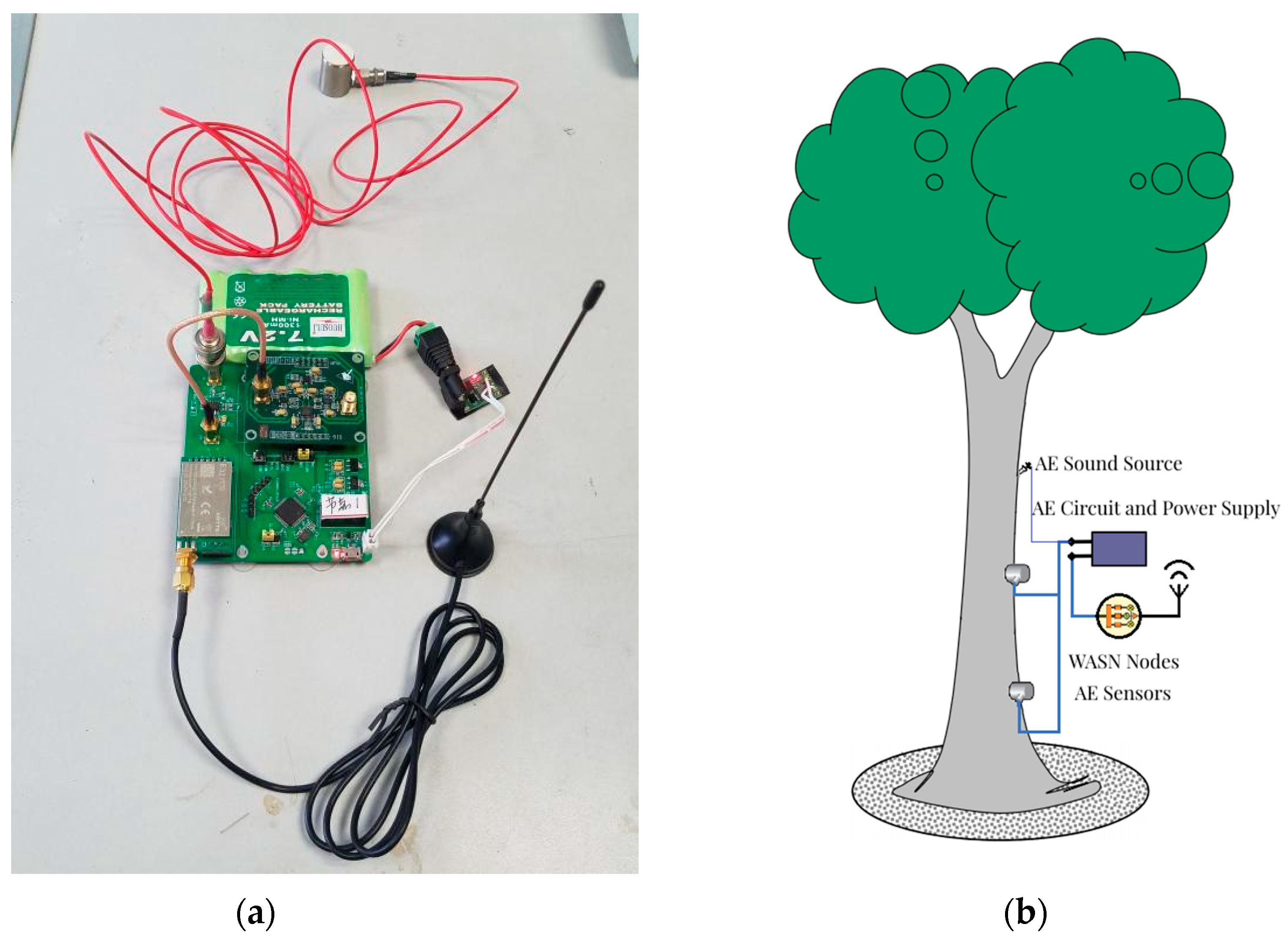
Figure 1. Schematic diagram of the basic architecture of forestry IoT system.
Forests 13 01879 g001
Figure 2. Framework of wireless AE node composition.
Forests 13 01879 g002
Figure 3. Sample wireless AE node and its installation measurement schematic. (a) Sample wireless AE node; (b) its installation measurement schematic.
Forests 13 01879 g003
Figure 4. AE data collection curve.
Forests 13 01879 g004
Figure 5. Example of single waveform acquisition results for near-end and far-end AE sensors. (a) A typical test waveform of Metasequoia trunk with 10% moisture content; (b) a typical test waveform of Metasequoia trunk with 20% moisture content.
Forests 13 01879 g005
Figure 6. Framework structure of WASN moisture content diagnosis method.
Forests 13 01879 g006
Figure 7. Basic structure of GAN model.
Forests 13 01879 g007
Figure 8. Basic structure of Conditional Tabular GAN (CTGAN) model.
Forests 13 01879 g008
Figure 9. Variation of loss values of generators and discriminators.
Forests 13 01879 g009
Figure 10. Kernel density estimation plots for the original AE feature dataset and the generated 1× data.
Forests 13 01879 g010
Figure 11. Cumulative and distribution of generated and real data.
Forests 13 01879 g011
Figure 12. CTWGAN-GP-L algorithm generates 3D maps of 1×, 2×, and 3× AE feature data, respectively. (a) 1× 3D color mapping surface map; (b) 2× 3D scatter plot; (c) 3× 3D bar chart.
Forests 13 01879 g012
Figure 13. Classification accuracy of the dataset with different mixing multipliers.
Forests 13 01879 g013
Figure 14. Physical view of sample data collection.
Forests 13 01879 g014
Figure 15. Calibration chart of moisture content of metasequoia wood samples.
Forests 13 01879 g015
Figure 16. Proximal/distal AE signal acquisition data for each wood sample. (a) Proximal AE amplitude; (b) distal AE amplitude; (c) proximal AE energy; (d) distal AE energy; (e) proximal AE duration; (f) distal AE duration.
Forests 13 01879 g016aForests 13 01879 g016b
Figure 17. Random Forests (RF) algorithm screening feature results.
Forests 13 01879 g017
Figure 18. Box plot of recognition accuracy for different number of feature variables.
Forests 13 01879 g018
Figure 19. GSCV-LGB program workflow diagram.
Forests 13 01879 g019
Figure 20. XGBoost algorithm filtering feature results.
Forests 13 01879 g020
Figure 21. Comparison of each evaluation metric of GSCV-LGB algorithm, GSCV-RF algorithm and GSCV-DT algorithm. (a) Precision comparison chart; (b) comparison chart of recall rate; (c) F1-score comparison chart; (d) MCC comparison chart; (e) ROC curve comparison chart; (f) confusion matrix of GSCV-LGB algorithm; (g) confusion matrix of GSCV-RF algorithm; (h) confusion matrix of GSCV-LGB algorithm.
Forests 13 01879 g021aForests 13 01879 g021b
Figure 22. Installation test chart and calibration chart of Zhejiang Nan and Triangle Maple. (a) Actual test of this WASN on Zhejiang Nan; (b) Actual test of this WASN on Triangle Maple; (c) Zhejiang Nan test moisture content calibration chart; (d) Triangle Maple test moisture content calibration chart.
Forests 13 01879 g022aForests 13 01879 g022b
Table 1. Generator network parameters.
Network LayerOutput ShapeParameter Value
Fully connected layer(None, 32)512
LeakyReLU(None, 32)0
BN layer(None, 32)128
Fully connected layer(None, 64)2112
LeakyReLU(None, 64)0
BN layer(None, 64)256
Fully connected layer(None, 128)8320
LeakyReLU(None, 128)0
BN layer(None, 128)512
Fully connected layer(None, 15)1935
Table 2. Discriminator network parameters.
Network LayerOutput shapeParameter Value
Fully connected layer(None, 32)512
LeakyReLU(None, 32)0
Dropout(None, 32)0
Fully connected layer(None, 64)2112
LeakyReLU(None, 64)0
Dropout(None, 64)0
Fully connected layer(None, 128)16,512
LeakyReLU(None, 128)0
Dropout(None, 128)0
Fully connected layer(None, 1)129
Table 3. Details of the Abalone dataset.
CategoryNumber of Each CategoryCategory Description
01528Males
11307Female
21342Juvenile
Table 4. Details of the image segmentation dataset.
CategoryNumber of Each CategoryCategory Description
1330Face tiles
2330Sky
3330Leaves
4330Cement
5330Window
6330Road
7330Grass
Table 5. Experimental environment.
Experimental ToolsVersion Number
Computer systemWindows 10 X64
GPUNVIDIA GeForce RTX 3090
Python (DE, USA)3.8.3
TensorFlow (San Francisco, CA, USA) 2.8.0
numpy (DE, USA)1.18.5
pandas (DE, USA)1.2.4
matplotlib (DE, USA)3.4.3
Table 6. Quality assessment of data generated by each algorithm.
DatasetAlgorithm ModelMMD1-NN
Generate 1× DataGenerate 1× Data
AbaloneSMOTE0.00090.7269
TGAN0.00140.6613
CTGAN0.00120.6219
CTWGAN-GP-L0.00070.5234
Image SegmentationSMOTE0.01210.9394
TGAN0.01320.6989
CTGAN0.01300.6382
CTWGAN-GP-L0.01190.5465
AE characteristic parametersSMOTE0.03930.8000
TGAN0.04160.7382
CTGAN0.04130.6954
CTWGAN-GP-L0.01710.5108
Table 7. AE feature screening results.
Filtering
Algorithm
AE Feature Quantity Merit Ranking
Random Forests (RF)①proximal/distal energy difference; ②proximal/distal amplitude difference; ③proximal amplitude; ④proximal energy; ⑤proximal/distal duration difference; ⑥proximal rise time; ⑦distal amplitude; ⑧distal rise time; ⑨distal ringing count; ⑩distal energy; ⑪proximal duration; ⑫ proximal ringing count; ⑬distal duration; ⑭proximal/distal rise time difference; ⑮proximal/distal ringing count difference.
Table 8. LightGBM results after XGBoost and RF feature screening.
Feature Selection MethodTest Results
Accuracy Rate (%)
XGBoost85.5
RF96.2
Table 9. Performance test results of each algorithm model.
Algorithm ModelTest Results
Accuracy Rate (%)Weighted Average
DT92.80.93
GSCV-DT93.90.94
RF93.50.94
GSCV-RF94.40.94
LightGBM96.20.96
GSCV-LGB97.90.98
Table 10. DT algorithm tuning results.
NameInitial ValueTuning Value
max_depth08
min_impurity_decrease00
min_samples_leaf11
Table 11. RF algorithm tuning results.
NameInitial ValueTuning Value
n_estimators511
max_features28
Table 12. LightGBM algorithm tuning results.
NameInitial ValueTuning Value
max_depth35
num_leaves86
subsample10.75
cosample_bytree0.80.65
reg_alpha51
reg_lambda101
Table 13. Confusion matrix of the results of the standing timber test.
Diagnosis AccuracyMagnoliaZelkovaTriangle MapleZhejiang NanGinkgo Yunnan Pine
Magnolia98.8%
Zelkova 98.7%
Triangle Maple 99.1%
Zhejiang Nan 97.5%
Ginkgo 98.2%
Yunnan Pine 97.4%
Publisher’s Note: MDPI stays neutral with regard to jurisdictional claims in published maps and institutional affiliations.