Article

The Current and Future Potential Geographical Distribution and Evolution Process of Catalpa bungei in China

1
College of Water Resources and Environment, Zhengzhou University, Zhengzhou 450001, China
2
Yellow River Institute of Hydraulic Research, Yellow River Conservancy Commission, Shunhe Road 45, Zhengzhou 450003, China
3
College of Water Conservancy Science and Engineering, Zhengzhou University, Science Road 100, Zhengzhou 450003, China
*
Author to whom correspondence should be addressed.
Forests 2022, 13(1), 96; https://doi.org/10.3390/f13010096
Submission received: 8 November 2021 / Revised: 5 January 2022 / Accepted: 6 January 2022 / Published: 10 January 2022
(This article belongs to the Section Forest Ecology and Management)

Abstract

:
Catalpa bungei C. A. Mey. (C. bungei) is one of the recommended native species for ecological management in China. It is a fast-growing tree of high economic and ecological importance, but its rare resources, caused by anthropogenic destruction and local climatic degradation, have not satisfied the requirements. It has been widely recommended for large-scale afforestation of ecological management and gradually increasing in recent years, but the impact mechanism of climate change on its growth has not been studied yet. Studying the response of species to climate change is an important part of national afforestation planning. Based on combinations of climate, topography, soil variables, and the multiple model ensemble (MME) of CMIP6, this study explored the relationship between C. bungei and climate change, then constructed Maxent to predict its potential distribution under SSP126 and SSP585 and analyzed its dominant environmental factors. The results showed that C. bungei is widely distributed in Henan, Hebei, Hubei, Anhui, Jiangsu, and Shaanxi provinces and others where it covers an area of 2.96 × 10 6 km 2 . Under SSP126 and SSP585, its overall habitat area will increase by more than 14.2% in 2080–2100, which mainly indicates the transformation of unsuitable areas into low suitable areas. The center of its distribution will migrate to the north with a longer distance under SSP585 than that under SSP126, and it will transfer from the junction of Shaanxi and Hubei province to the north of Shaanxi province under SSP585 by 2100. In that case, C. bungei shows a large-area degradation trend in the south of the Yangtze River Basin but better suitability in the north of the Yellow River Basin, such as the Northeast Plain, the Tianshan Mountains, the Loess Plateau, and others. Temperature factors have the greatest impact on the distribution of C. bungei. It is mainly affected by the mean temperature of the coldest quarter, followed by precipitation of the wettest month, mean diurnal range, and precipitation of the coldest quarter. Our results hence demonstrate that the increase of the mean temperature of the coldest quarter becomes the main reason for its degradation, which simultaneously means a larger habitat boundary in Northeast China. The findings provide scientific evidence for the ecological restoration and sustainable development of C. bungei in China.

Graphical Abstract

1. Introduction

Vegetation is the basis of the ecosystem, which plays an important role in energy exchange, biogeochemical cycle, and hydrological cycle on the land surface. The distribution of vegetation is limited by anthropogenic and natural environmental factors, such as anthropogenic disturbance, climate, underlying surface characteristics, and others [1,2]. Climate has become one of the dominant factors influencing the geographic distribution patterns of vegetation at the regional and global scales [3,4]. It turns out that global climate change, especially climate extremes, has significantly impacted terrestrial ecosystems over the past century [3,5,6]. The assessment report of the IPCC AR6 concluded that global warming has continued to intensify mainly due to human activities, and the frequency and intensity of extreme climate events increase as well [7], which would lead to enormous vegetation changes. Climate changes potentially induce marked vegetation disequilibrium with climate at both leading and trailing edges [8]. It has been found that climate change has led to loss and fragmentation of vegetation habitat [9,10,11]. For example, the climatically suitable range of about 57% of widely distributed plant species is expected to be reduced by more than 50% at maximum by 2080 due to climate warming [12]. Inadequate understanding of the impact of climate change on vegetation brings about a particularly difficult challenge for foresters and ecologists. For this reason, it is of great significance to explore vegetation distribution under climate change, reveal its formation and migration characteristics, and develop countermeasures for restoration and conservation.
Species distribution models (SDMs) have become important tools to discover the effects of climate change on species during the last two decades [13,14]. SDMs can simulate the basic niche of species based on the dependence of species on environmental factors and obtain the habitat suitability of species [15]. An increasing number of scholars apply SDMs to the fields related to the relationship between species and climate change, such as assessment of biological invasion risks [16], conservation of endangered species [17], and the research of species’ vulnerability to climate change [18]. Maximum entropy model (Maxent) [19] has become one of the most commonly used SDMs for years, which has the advantages of less requirement of sample size and category, flexible variable processing, and excellent simulation effect [20,21]. Zhang et al. (2021) established Maxent and prioritizr models to simulate the potential distribution of 60 native species in the Yanhe River catchment [22]. Dyderski et al. (2018) predicted most of the species studied that would face a significant decrease in suitable habitat area under the assumptions of limited migration [9]. Lim et al. (2018) found that warm temperate evergreen forest shows distinctive northward migration and substantial increase, and subalpine forest areas and regions with high diversity decreased due to climate change [23].
Catalpa bungei C. A. Mey., the genus Catalpa Scop. of the Bignoniaceae family, is widely distributed in the Yellow River Basin, and is one of the top ten recommended species for ecological management due to its well-developed root system and strong resistance to wind and soil [24]. It has been listed by The State Forestry Administration as a precious tree in North China for vigorous promotion and increasing in recent years [25]. Harder generative reproduction has limited its development, while vegetative propagation techniques and breeding of fine varieties are commonly applied to accelerate its reproduction [26,27]. The natural germplasm resources of C. bungei have become scarce due to forest destruction [28], and it is mostly scattered plantations with little natural wild distribution [29]. However, as the key to alleviate the contradiction of supply–demand for its domestic resources [30], its large-scale planting should also consider long-term environmental suitability. It has been proven that large-scale afforestation, such as Hippophae rhamnoides L. and Robinia pseudoacacia L., causes serious soil dry layer on the Loess Plateau, which increases the risk of ecosystem vulnerability [31]. Therefore, unreasonable afforestation may exacerbate local resource conflicts and damage ecological balance, or scarcely achieve its sustainable development. As for C. bungei, it has been observed that some problems, such as its local degradation, less production, and ecological quality, have become serious according to the survey of Henan Forestry Bureau. To reduce or avoid these risks of environmental resource conflicts, revealing the mechanism of interaction between species distribution and environment is beneficial to forest cultivation and selection. However, the selection of afforestation land in China mostly depended on the current climate with little considering of its climate adaptability [32], which easily leaves behind great threats to degradation, less production quality, and even extinction for trees highly sensitive to climate change. For C. bungei, though it has been widely recommended for ecological management, the impact mechanism of climate change on its growth has not been studied yet. Therefore, it is urgent to explore C. bungei’s response to climate change, reveal climatic factors that probably cause local degradation, and identify stable habitats for its restoration and management.
Based on different environmental factors and multiple model ensemble (MME) of CMIP6, the study applied Maxent to forecast C. bungei’s potential distribution under different climate scenarios, which aimed to research the following: (1) Constructing the optimal Maxent of C. bungei, determining the current and future distribution and area variation of different grades of suitable areas and analyzing its dominant factors; (2) Using the migratory direction of C. bungei to estimate its adaptive capacity to climate change from 2021–2040, 2041–2060, 2061–2080, and 2081–2100 under the climate scenarios of SSP126 and SSP585.

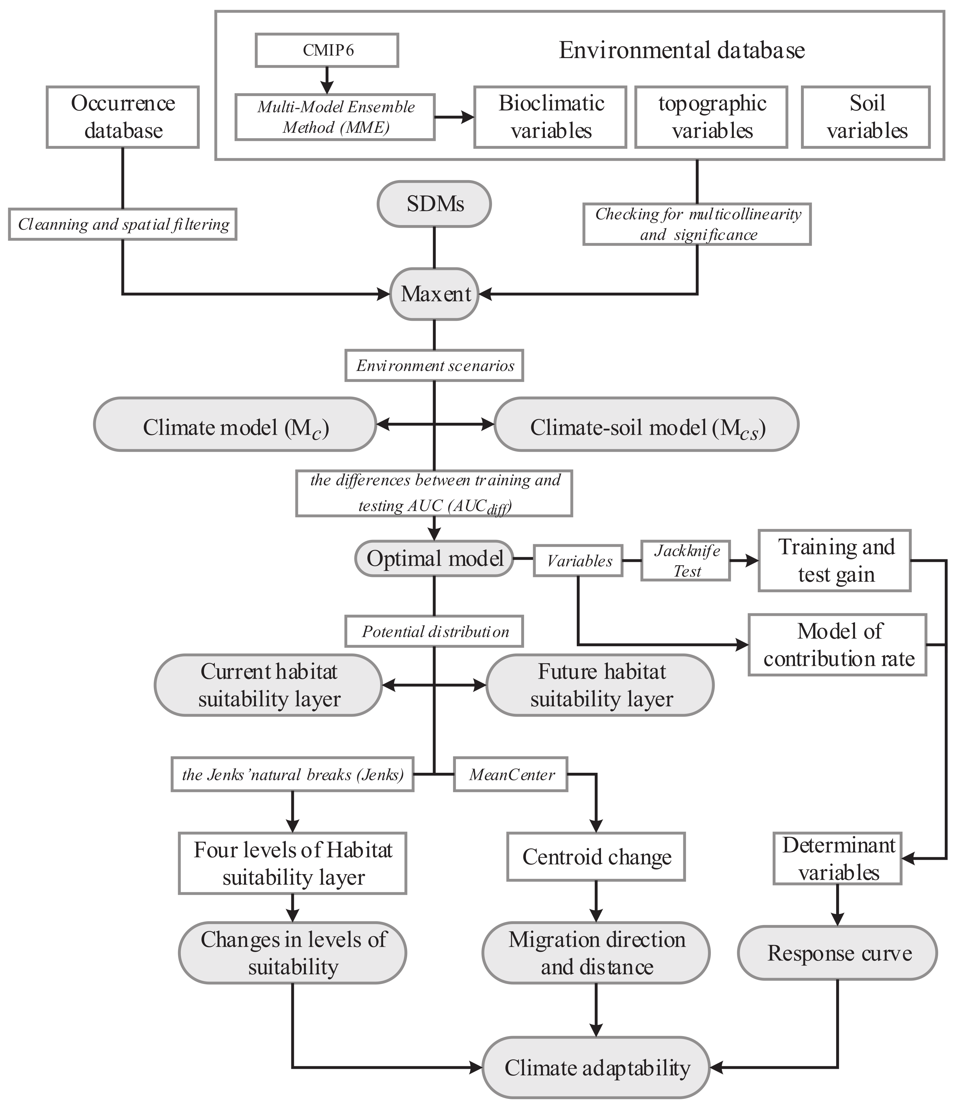
2. Materials and Methods

2.1. Collecting Species Occurrence Data

The occurrence records of C. bungei mainly come from the Global Biodiversity Information Network Database (GBIF; https://www.gbif.org (accessed on 11 September 2021)), the National Specimen Information infrastructure (NSII; http://www.nsii.org.cn (accessed on 11 September 2021)), and the Chinese Plants Image database (http://www.plantphoto.cn (accessed on 11 September 2021)). We identified and eliminated invalid and duplicate records, and then sampled points diluted by spatial filtering to avoid the influence of sampling bias on model output [33,34]. Finally, we obtained 43 distribution points.

2.2. Environmental Data

The climate dataset used in the study was downloaded from the World Climate Database (http://www.worldclim.org (accessed on 20 September 2021)) [35]. We adopted one past climate data for 1970–2000 (1 km 2 ) and nine future global climate models (GCMs) of CMIP6, with a spatial resolution of 2.5 arc-minutes (approximately 4.5 km 2 ). Refer to literature for assessment of GCMs applicability in China [36,37,38]. Those climate models with poor simulation were excluded, while the remaining were used to obtain the climate model (MME) by mean of multimodel ensemble method [39]. MME included BCC-CSM2-MR, CNRM-CM6-1, MIROC-ES2L, and MRI-ESM2-0 (Table 1)). Each model includes different shared socioeconomic pathways (SSPs) in future periods (2021–2040, 2041–2060, 2061–2080, 2081–2100), e.g., low emission scenario SSP1-2.6 (referred to as SSP126) and high emission scenario SSP5-8.5 (SSP585). Three topographical variables, e.g., altitude (Alt), slope (Slp), and aspect (Asp) are extracted by DEM downloaded from Geospatial Data Cloud (http://www.gscloud.cn (accessed on 20 September 2021)). Soil variable (http://www.resdc.cn (accessed on 20 September 2021)) is a raster of soil type generated digitally from the “1:1 Million Soil Map of the People’s Republic of China” compiled and published by the National Soil Survey Office in 1995 (Table 1). As collinearity shift and environmental novelty can negatively affect Maxent transferability [40], variables partly with high collinearity that lead to model complexity and overfitting were then selected in part by Pearson’s correlation statistic [41,42] (Table 2). Ten independent variables with greater ecological significance and more environmental information were adopted after only one variable was kept for further analysis in each set of significantly cross-correlated variables (r≥ 0.8) [22]. After that, their importance regarding the influence on the distribution of C. bungei was preliminarily analyzed by the jackknife approach, and the variables such as asp and slp with little importance were excluded. Finally, all environmental variables were selected by three evaluation principles (Table 3) to obtain the predictor data set VS 4 (Table 4).

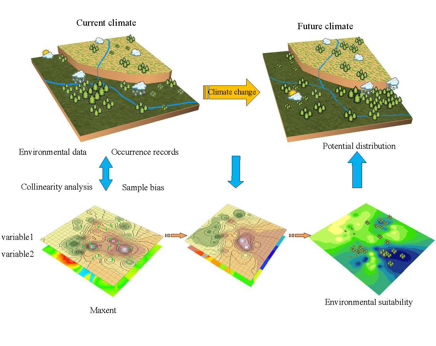
2.3. Construction and Validation of Maxent

The software of Maxent (V3.4.4) [43] was applied to analyze the suitability of C. bungei under climate change. To verify the generalization of models, we introduced different scenarios of “climate” and “climate-soil” that consist of 43 distribution records and 9 variables into models for further determining appropriate generalization models, and we constructed the climate model (M C ) and climate-soil model (M C S ). In modeling, K-fold cross validation (K-CV) was repeated 10 times (K = 10) so that each subsample could participate in training and testing to reduce generalization error [44], while other parameters defaulted. Then, the jackknife approach was used to examine training and test gain of the selected variables to analyze the dominant climate factors [45]. Finally, we took the area under the curve (AUC) for receiver operating values that are independent of judgment thresholds as the indicator of model prediction accuracy [46]. The closer AUC is to 1, the better a model performs. The evaluation criteria of AUC is as follows: fail (0.5–0.6), poor (0.6–0.7), fair (0.7–0.8), good (0.8–0.9), and excellent (0.9–1.0) [42]. Response curves were used to study the relationships between variables and the predicted probability of the presence of C. bungei.
According to the Jenks natural breaks (Jenks), the index of habitat suitability from the models was reasonably divided into the following four levels: unsuitable area (0–0.12), low suitable area (0.12–0.36), middle suitable area (0.36–0.65), and high suitable area (0.65–1). We calculated the suitable area of C. bungei through the grid calculator of ArcGIS 10.5, superimposed current and future grid maps of suitable areas to summarize the level and range change of distribution over time, and draw its levels as the degraded, enhanced, and stable area. At the same time, we analyzed the trends of dominant environmental factors in different regions and calculated the average center of suitable areas under different climate scenarios. Then, we drew the migration road of C. bungei by connecting each average center in a time series to obtain its migrated direction and distance. The specific analysis process of the study is shown in Figure 1.

3. Results

3.1. Comparison and Evaluation of Maxent under Current Climate

The AUC t r a i n i n g of M C and M C S is 0.926 and 0.947 and their AUC t e s t is 0.894 and 0.887, which means these models both perform with good accuracy (Figure 2). However, the M C S performed the lowest training error but largest generalization error, and it is not suitable for large-scale prediction. Due to the smaller difference between training and testing AUC (AUC d i f f ), M C was used as the final potential distribution model of C. bungei, which shows that the suitable area is about 2.96 × 10 6 km 2 under current climate conditions. High suitable areas are mainly distributed in Henan, Hebei, Hubei, Anhui, Jiangsu, and Shaanxi provinces, and partly located in the Shandong Peninsula, Gansu, and the north part of the Zhejiang and Yunnan provinces. The section of the North China Plain in Shandong province, Hunan, Guizhou, Sichuan, and Yunnan provinces and the hills of Shandong have the most middle suitable areas, There are low suitable areas mostly in Fujian, Jiangxi, Sichuan, Guizhou, the north part of Yunnan, the south part of Liaoning provinces, and the northwest of the Loess Plateau, and partially in the northwest of Tibet province (Figure 3).

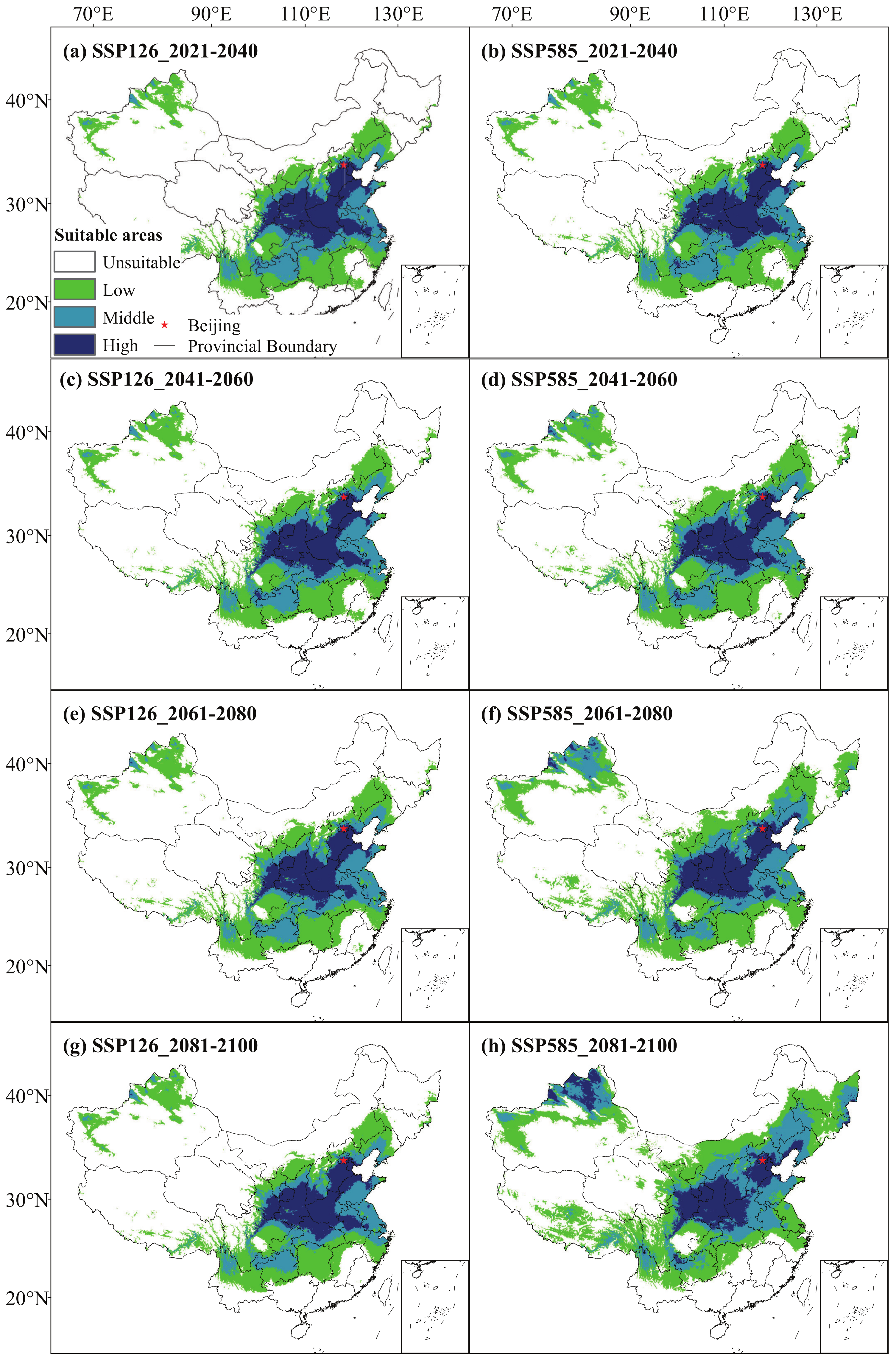
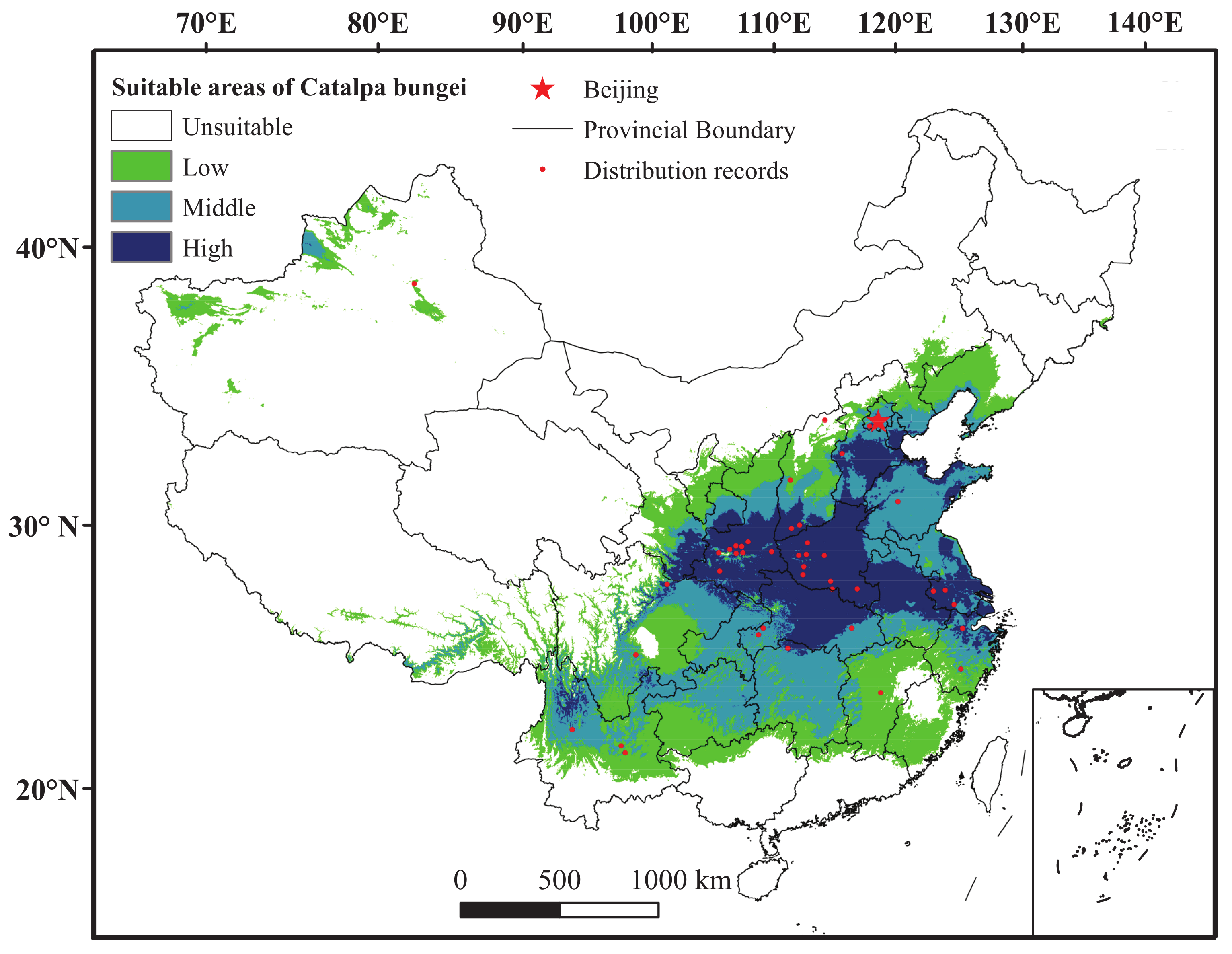
3.2. Potential Distribution of C. bungei under Future Climate

Under SSP126, the suitable areas of C. bungei generally showed an increasing trend, with a total increase of 0.42 × 10 6 km 2 (14.2%) by 2100 (Figure 4, Table 5). The high suitable areas continued to decline in 2041–2080, but its overall area remained basically unchanged by 2100. Except from 2041 to 2060, the middle suitable areas decline at an average rate of only 3%. Compared with the former, the low suitable areas increase obviously by 50%, which mainly indicate the transformation of unsuitable areas into low suitable areas. Under SSP585, the area of each area changed more violently, which mainly manifested in the increase of high, middle, and low suitable areas. Except for individual periods, they basically maintain the growth trend, with a total increase of 15.71%, 41.28%, and 105.13%, respectively.
The change in habitat classes during four periods under SSP126 and SSP585 was used as the basis for mapping the growth subregions of C. bungei to determine its distribution trends (Figure 5). Under SSP126 and SSP585, the middle and high suitable areas are basically consistent with the corresponding existing zones distributed in Shaanxi, Henan and the north of Hunan, Shandong, and Jiangsu. The degraded areas are located discretely and widely in Hunan, Jiangxi, Zhejiang, the south-central of Anhui, the south of Hubei, the north of Jiangsu, and the south of the Yangtze River. There are weakly degraded areas mainly in the southern areas at low latitudes at the edges of the middle and high suitable areas, while the strongly degraded areas are distributed in the south of Anhui, Hubei and Jiangsu, and the north of Zhejiang under SSP585. As for distribution areas in most regions, the enhancement areas are located in the Loess Plateau, the Haihe Plain, and the north of the Yellow River Basin. Compared to SSP126, the more suitable areas become larger, and the new formation will occur in the Northeast Plain, the Junggar Basin, the Tianshan Mountains, and the Changbai Mountain under SSP585.
The center of the suitable areas for C. bungei is located at the location (32.3 ° N, 110.2 ° E) (Figure 6). Under SSP126, it will move 2.19 × 10 5 m and 0.55 × 10 5 m, respectively, in 2021–2040 and 2041–2060, with a tendency to fast migration to the northwestward but relatively and slowly after that. The total longitudinal and latitudinal offset of the migration was 1.77 ° and 2.25. Under SSP585, the characteristic of migration for C. bungei was significantly different from that of SSP126. With the distance of migration greater than 1 × 10 5 m in each period, the total longitudinal and latitudinal offset reaches approximately 2.7 ° and 4.76 ° by 2100, which leads to the relocation of the center to the north of Shaanxi province (37.05 ° N, 107.46 ° E). According to the change of migration rate, it decreases with time and reaches the minimum of 0.1 × 10 5 m in 2081–2100, and the migration direction shows a trend of migration to low latitudes under SSP126. Under SSP585, the migration rate increases slowly in the latter three periods, showing a trend of continuous movement to the northwest in the future.

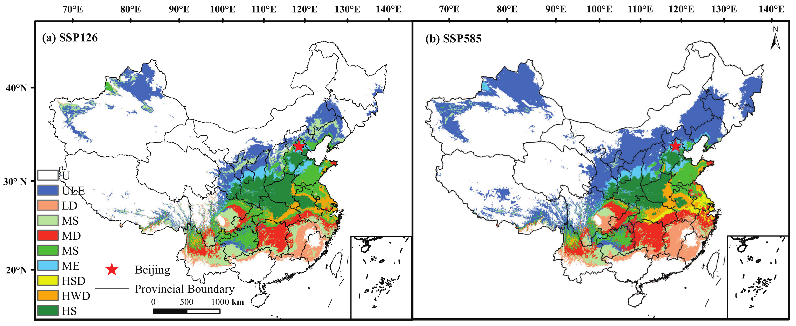
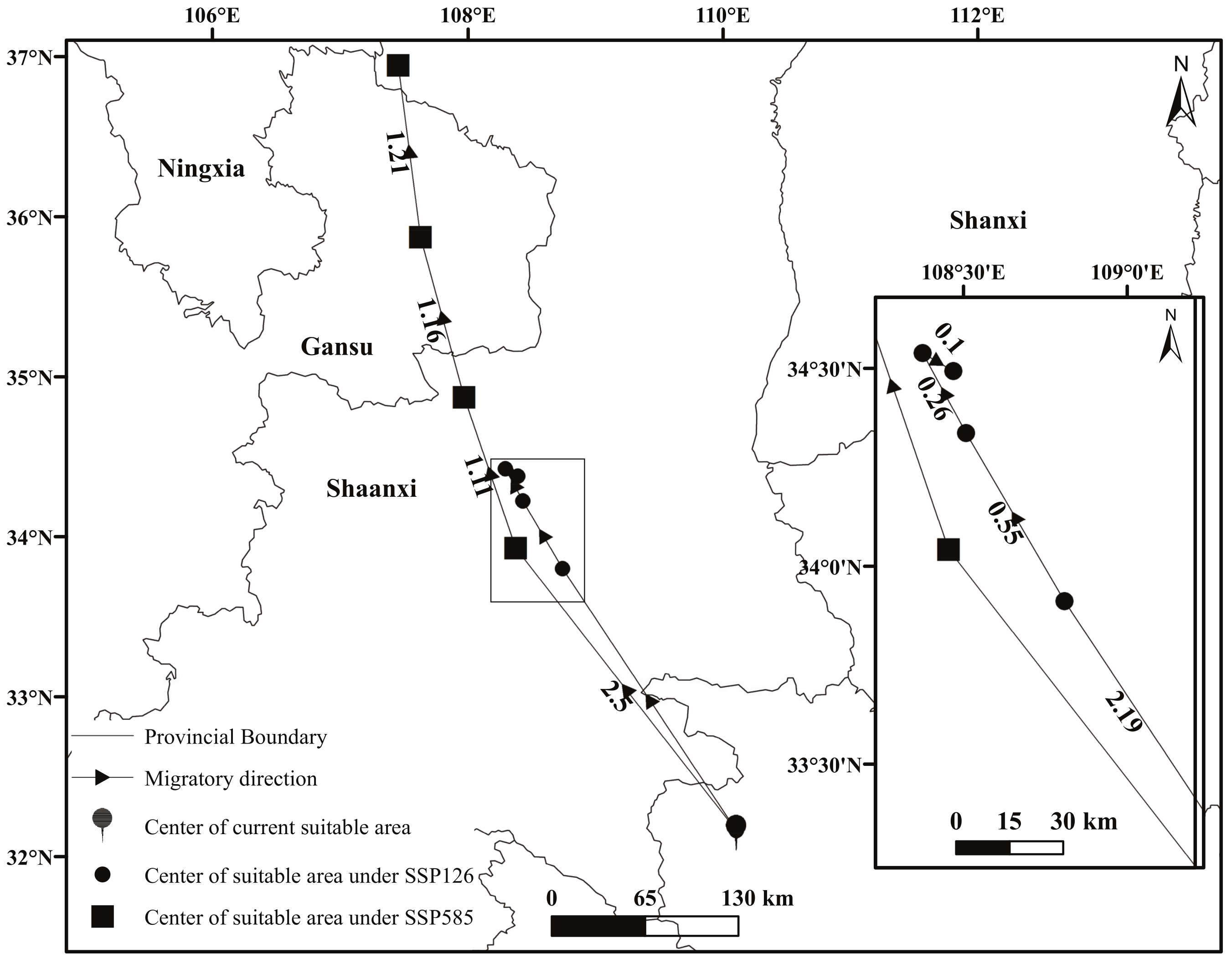
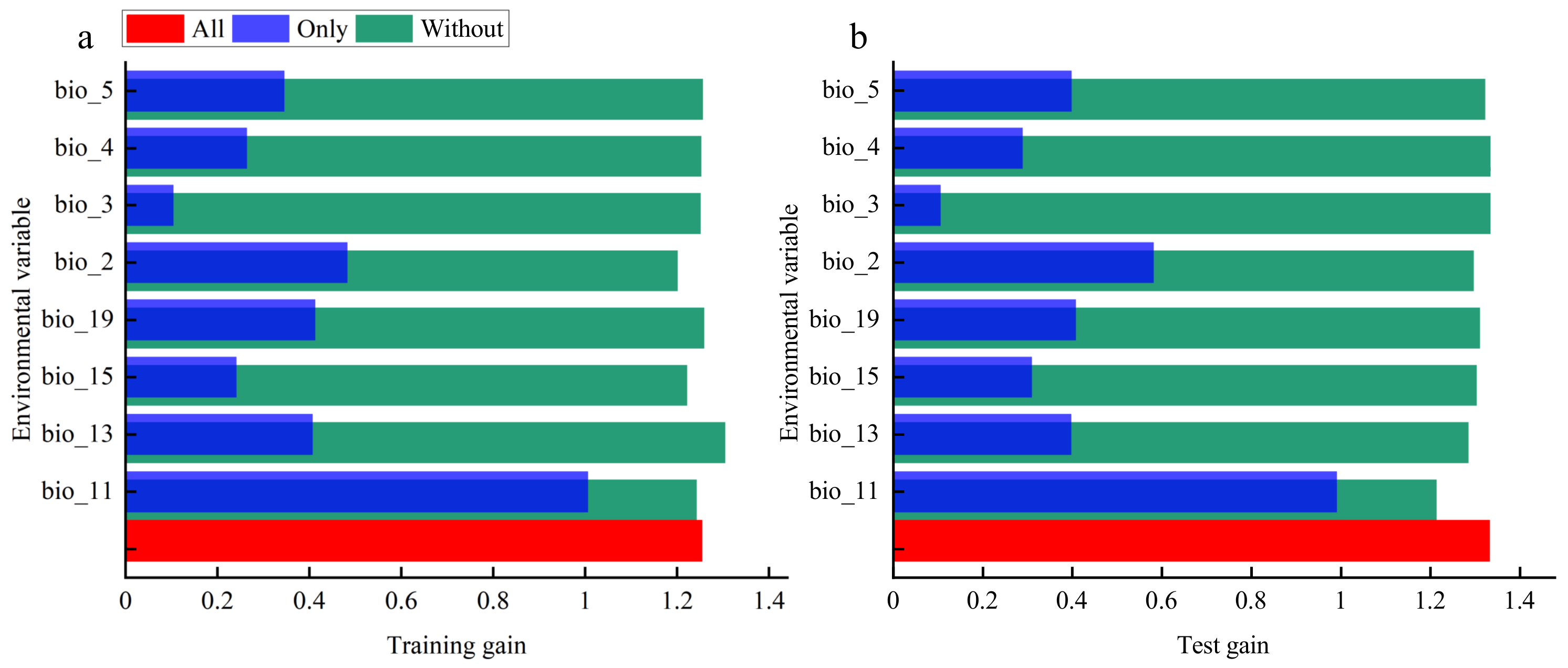
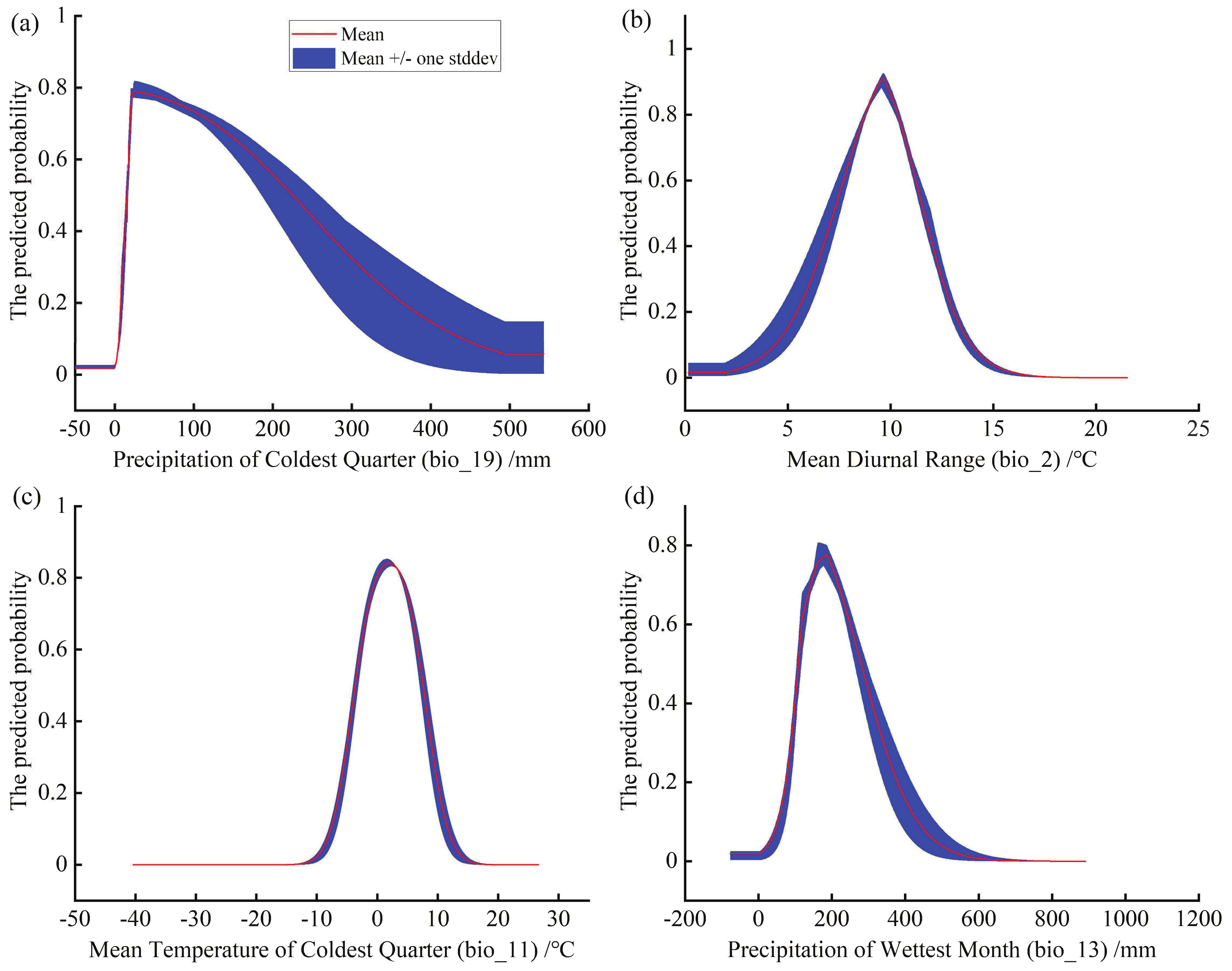
3.3. The Dominant Environmental Factors Influencing Potential Distribution of C. bungei

The results of variable contribution and permutation importance showed that bio_11 had the greatest importance, followed by bio_13, bio_19, bio_15 and bio_2 (Table 6). The jackknife test showed the variables were basically the same in model training and testing gain, with bio_11 having the highest training gain, followed by bio_13, bio_2, and bio_19 (Figure 7), indicating that bio_11, bio_13, bio_2, and bio_19 had the greatest influence on distribution of C. bungei.
The climate response curve represents the relationship between variables and habitat (Figure 8). Taking the suitable growth probability p > 0.5 as an example, C. bungei is in the best growth condition when the mean temperature of the coldest quarter is −3.62–7.57 ° C and the range of precipitation of the wettest month is 109.1–279.32 mm. In addition, the mean diurnal range should be 7.24–11.64 ° C, and precipitation of the coldest quarter should be 15.2–225 mm. The variation of dominant factors in each growth subregion is comparatively obvious (Table 7), with the mean temperature of the coldest quarter in the degraded, stable, and enhanced zones being around 5–10 ° C, 3–4 ° C, and below 0 ° C, mean diurnal range being around 8–9 ° C, 10 ° C, and 11–12.5 ° C, respectively. Mean temperature of the coldest quarter in the degraded zones was significantly larger than that in other zones, indicating that the increase of mean temperature of the coldest quarter was one of the main reasons for the degradation of C. bungei. The range of mean temperature of the coldest quarter in different periods within the single zone is above 2 ° C, and the variation of precipitation of wettest month is above 10 mm. The variation means that the temperature of coldest quarter becomes larger, while that of the mean diurnal range becomes smaller under SSP585, which indicates that each growing subregion under climate change is mainly affected by the variation of the mean temperature of the coldest quarter.

4. Discussion

4.1. Model Evaluation

In this study, we use MME of CMIP6 with better applicability in China compared to CMIP5 to set different scenarios to predict the distribution of C. bungei [36], which somewhat also reduces uncertainty relative to a single model [39,46]. In addition to climate, species distribution depends on many factors including topography, soil, interspecies relationships, species evolution, and human activity [47]. Many past studies have adopted only climate factors in modeling that fail to describe in all their complexity the processes that limit species’ ranges [48]. Though those models perform well, the inferred niche may be far away from its basal niche with misleading predictive risk [49]. Topography variables associated with hydrothermal conditions might have a great influence on the distribution of species [50,51,52]. Therefore, non-climate variables should be included in the scope of model prediction factors if obtained when their significance remains vague. To avoid loss of the key information, we considered climate, topography, and soil variables for the identification of which kind of variables contribute to better prediction. In the study, topographic factors that we took initially into account were excluded by their high collinearity with climate and little significance of models. Therefore, we only constructed M C and M C S , and the results showed that M C indicated more excellent model performance than M C S by checking for smaller AUC d i f f . Soil type could improve AUC t r a i n i n g but might lead to large randomness and overfitting with detriment to model generalization. The previous study had shown that C. bungei requires lower soil conditions and can grow in ordinary soil, similar to a limestone mountain with less soil and barren arid shale soil [53], which confirms soil type is not the key limiting factor and not suitable for analysis. Therefore, we take M C as the best model to reduce model uncertainty.

4.2. Key Environmental Variables and Current Spatial Distribution

Hydrothermal conditions are the main abiotic factors that determine the spatial distribution of vegetation [54,55]. M C indicated that mean temperature of the coldest quarter (bio_11), precipitation of the wettest month (bio_13), precipitation of the coldest quarter (bio_19), and mean diurnal range (bio_2) play important roles in constraining the potential distribution of C. bungei. The bio_11 controls its northern boundary, and its growth was significantly regulated by bio_13 in the rainy season when C. bungei reaches 64.2% of the annual growth [56], which confirms the statement of its intolerance of moisture and cold [57,58]. Aside from average temperature, bio_19 will further restrict its growth in winter, and bio_2 held the main constraint for its growth throughout the year. Previous studies have shown that C. bungei is suitable for climate conditions with a mean annual temperature of 10–15 ° C and annual precipitation of 500–1000 mm [56]. However, the effects of extreme climate events on terrestrial vegetation activities are often more severe than long-term changes in the mean climate [59,60], and the seedlings of C. bungei are vulnerable to freezing damage of extremely low temperature in the early stage of growth [56]. In addition, C. bungei can adapt to drought conditions because of its lower water consumption and lower transpiration water consumption rate [60,61], which is similar to the conclusion of bio_19 of 15.2–225 mm. Therefore, we thought these extreme climatic variables in the study could be more conducive to the response of C. bungei to increase extreme climate events.
The study indicated that the core areas of C. bungei are mainly distributed in Shandong Hills, Henan, Hubei, Shaanxi, Jiangsu, Hunan, and the section of the North China Plain in Hebei, which is basically consistent with the conclusions of previous studies [53]. There are eastern core areas close to continuous middle suitable areas, the southern part of widely distributed low suitable areas in the Yangtze River Basin, and northern suitable areas relatively small due to the low temperature generated by the high altitude.

4.3. Potential Distribution of C. bungei under Future Climate

Under SSP126 and SSP585, the increase of mean temperature of coldest quarter drives the migration of C. bungei to the north and expands low suitable areas by more than 50%. The middle and high suitable area basically remains stable under SSP126, but increases by above 40% and 15%, respectively, under SSP585. The center of distribution has an obvious indigenous movement and will transfer from the junction of Shaanxi and Hubei to the north of Shaanxi. By the end of the 21st century, temperature and precipitation would increase, especially in high-altitude areas such as Western and Northern China, where they increase the fastest [36]. In that time, elevated temperature leads to prolonged growing seasons and increased vegetation activity in Northern China [62], which may be the reason for its expanding into northeast China and decrescent original habitats. The climate scenario of SSP585 has the greatest impact on its habitats such that most suitable areas degenerate in the south of the Yangtze River Basin, especially in Anhui, Hubei, and Jiangsu, but tend to strengthen in the Loess Plateau, Haihe Plain, and the north of the Yellow River Basin. Li et al. (2015) used the classical Holdridge life zone model to assess vegetation zone responses to climate change, which also suggests that future climate change will contribute to the growth and expansion of forest zones on the Loess Plateau [63]. The stable habitats are located in warm-temperature areas such as the south of Shaanxi and Hebei and the north of Hubei and Henan. In general, the results show the increase of overall suitable area and migration to high latitudes of middle and high suitable areas. Consistent with most studies, warming will result in migration of species to higher latitudes [64,65], and the rate of northward migration is positively associated with the degree of warming [66,67].
The migration predicted in the study is only based on the response of C. bungei to climate change and does not consider geographical barriers, dispersal ability, and other factors which might cause smaller actual habitat than expected. Migration ability is an important factor influencing species adaptation to future climate change [68], and it is limited by competition from existing plant communities, anthropogenic habitat fragmentation, and loss of dispersal agents [69]. For example, the fragmented habitat of vegetation community in the Loess Plateau obviously limited vegetation diffusion [70]. Therefore, vegetation would degenerate locally when hydrothermal conditions under climate change cannot meet its growth hydrothermal conditions, which finally suffer from the risk of habitat reduction [71]. Although its habitats increase in this study, its vulnerability to climate change may also depend on whether it could adapt to climate change and new interspecies interactions via diffusion [72,73], which remains to be further discussed.

4.4. The Distribution of Plantation and Its Growth Subregions

Due to increased demand of ecological management in the Yellow River Basin and lack of market supply, China has established several artificial bases for the rapid development of Catalpa bungei plantations. Its artificial forests are mainly distributed in Taihang Mountain in Henan province, Luanchuan city, Henan province, Guiding city, Guizhou province, and others [57,58,74,75] (Table 8). Under the current climate, all the artificial forests belong to the suitable areas.
According to the characteristics of dominant factors of each base for C. bungei plantation (Table 9), it can be seen that the increase of low mean temperature of the coldest quarter leads to improved suitability. Mean diurnal range and precipitation of the coldest quarter in the Taihang Mountain in Hebei province are outside the optimum range, indicating that these two factors limit the growth of C. bungei, mainly due to its lower rainfall in the dry season and large temperature difference in high altitude, while the dominant factors in other regions are basically maintained in a better suitable range. The mean temperatures of the coldest quarter of Taihang Mountain in Hebei province, Yantai, and Qixia in Shandong province are the lowest relative to others, which indicates good adaptability to temperature rise, and those in Lijiang, Yunnan province, Jingmen, Hubei province, and Xingren, Guizhou province range from 6 to 8.3 ° C, which is close to the upper limit of the appropriate range. The Hengduan Mountains are widely distributed in Lijiang, Yunnan province; the complex climate change causes coexistence of degradation and enhancement, which is mainly reflected in the strengthening of the suitability of high-altitude mountains and degeneration in Canyon areas. Other bases have maintained good stability. In addition, Funiu Mountain and Dabai Tongbai Mountain in Henan province (high-stable zone) has become one of the construction project plans of Henan Forestry Ecological Province in recent years [76], an area which also turns out to have long-term significance of its construction base.

5. Conclusions

C. bungei, widely distributed in Henan, Hebei, Hubei, and Shaanxi provinces, is the most sensitive to temperature factors. Under future climate change, the increase of mean temperature of the coldest quarter leads to its migration to the north and increases the habitat areas. There are large areas of degradation in the south of the Yangtze River, while the more suitable areas are in the north of the Yellow River Basin. In addition to climate factors, human activities, such as artificial planting and land occupation, may also lead to habitat loss and fragmentation of C. bungei. The occupation of the best appropriate areas of C. bungei should be avoided. Therefore, the construction of C. bungei plantations should be undertaken in Henan, Shaanxi, and Shandong provinces as the main planting areas to ensure ecological restoration and sustainable development. In addition, it is necessary to develop appropriate protection policies based on the climatic and topographical characteristics of different suitable areas. For example, there are fragmented habitats, especially in the Loess Plateau, where the most suitable areas are distributed that should reduce human interference and establish natural reserves, such as Funiu Mountain, Dabie Mountain, and Taihang mountain. Artificial afforestation should avoid low-lying areas with ponding, or ensure smooth flood discharge. Understory vegetation or mixed vegetation shall be appropriately increased, especially in the suitable areas for returning farmland to forest area and desert where little surface vegetation leads to larger temperature differences, and tree thermal insulation measures shall be increased in cold years or areas in winter. In this paper, we studied the current and future distribution to determine the adaptability of C. bungei to climate change, but its adaptability could be further reduced due to multiple factors such as human activities, diffusion restrictions, and biological interaction. In future discussion, a more accurate distribution pattern would be obtained by combining these factors.

Author Contributions

Conceptualization, S.J. and T.Z.; methodology, S.J.; software, T.Z. and J.W.; validation, S.J. and D.Y.; formal analysis, J.W. and T.Z.; investigation, S.J., J.W., and D.Y.; resources, T.Z. and J.W.; data curation, S.J. and T.Z.; writing—original draft preparation, S.J.; writing—review and editing, T.Z. and D.Y.; visualization, J.W.; supervision, S.J. and D.Y.; project administration, S.J.; funding acquisition, S.J. and D.Y. All authors have read and agreed to the published version of the manuscript.

Funding

This research was funded by the National Key Research Priorities Program of China (2017YFC0404402), the Henan Natural Science Fund (212300410413), the Henan Youth Talent Promotion Project (2021HYTP030) and China Postdoctoral Science Foundation (2020M672247).

Institutional Review Board Statement

Not applicable.

Data Availability Statement

The data could be provided by the authors if necessary.

Acknowledgments

We thank Aoxue Wang, Qiankun Zhang, and Xueli Zhang from Zhengzhou University, and other municipal and county forestry investigators for their assistance in field collecting and analyzing species occurrence data and environmental data, as well as four anonymous reviewers for their very helpful suggestions.

Conflicts of Interest

The authors declare no conflict of interest.

References

  1. Çoban, H.O.; Örücü, Ö.K.; Arslan, E.S. MaxEnt Modeling for Predicting the Current and Future Potential Geographical Distribution of Quercus libani Olivier. Sustainability 2020, 12, 2671. [Google Scholar] [CrossRef] [Green Version]
  2. Arslan, E.S.; Akyol, A.; Örücü, Ö.K.; Sarıkaya, A.G. Distribution of rose hip (Rosa canina L.) under current and future climate conditions. Reg. Environ. Chang. 2020, 20, 107. [Google Scholar] [CrossRef]
  3. Moritz, C.; Agudo, R. The future of species under climate change: Resilience or decline? Science 2013, 341, 504–508. [Google Scholar] [CrossRef]
  4. Varol, T.; Canturk, U.; Cetin, M.; Ozel, H.B.; Sevik, H. Impacts of climate change scenarios on European ash tree (Fraxinus excelsior L.) in Turkey. Forest Ecol. Manag. 2021, 491, 119199. [Google Scholar] [CrossRef]
  5. Reichstein, M.; Bahn, M.; Ciais, P.; Frank, D.; Mahecha, M.D.; Seneviratne, S.I.; Zscheischler, J.; Beer, C.; Buchmann, N.; Frank, D.C. Climate extremes and the carbon cycle. Nature 2013, 500, 287–295. [Google Scholar] [CrossRef]
  6. McDowell, N.G.; Allen, C.D.; Anderson-Teixeira, K.; Aukema, B.H.; Bond-Lamberty, B.; Chini, L.; Clark, J.S.; Dietze, M.; Grossiord, C.; Hanbury-Brown, A. Pervasive shifts in forest dynamics in a changing world. Science 2020, 368, 964. [Google Scholar] [CrossRef] [PubMed]
  7. Working Groups—IPCC. 2021. Available online: https://www.ipcc.ch/working-groups (accessed on 1 November 2021).
  8. Svenning, J.C.; Sandel, B. Disequilibrium vegetation dynamics under future climate change. Am. J. Bot. 2013, 100, 1266–1286. [Google Scholar] [CrossRef] [PubMed]
  9. Dyderski, M.K.; Paź, S.; Frelich, L.E.; Jagodziński, A.M. How much does climate change threaten European forest tree species distributions? Glob. Chang. Biol. 2018, 24, 1150–1163. [Google Scholar] [CrossRef]
  10. Román-Palacios, C.; Wiens, J.J. Recent responses to climate change reveal the drivers of species extinction and survival. Proc. Natl. Acad. Sci. USA 2020, 117, 4211–4217. [Google Scholar] [CrossRef]
  11. Koo, K.; Park, S.; Seo, C. Effects of Climate Change on the Climatic Niches of Warm-Adapted Evergreen Plants: Expansion or Contraction? Forests 2017, 8, 500. [Google Scholar] [CrossRef] [Green Version]
  12. Warren, R.; VanDerWal, J.; Price, J.; Welbergen, J.A.; Atkinson, I.; Ramirez-Villegas, J.; Osborn, T.J.; Jarvis, A.; Shoo, L.P.; Williams, S.E.; et al. Quantifying the benefit of early climate change mitigation in avoiding biodiversity loss. Nat. Clim. Chang. 2013, 3, 678–682. [Google Scholar] [CrossRef] [Green Version]
  13. Pecchi, M.; Marchi, M.; Burton, V.; Giannetti, F.; Moriondo, M.; Bernetti, I.; Bindi, M.; Chirici, G. Species distribution modelling to support forest management. A literature review. Ecol. Model. 2019, 411, 108817. [Google Scholar] [CrossRef]
  14. Booth, T.H. Species distribution modelling tools and databases to assist managing forests under climate change. For. Ecol. Manag. 2018, 430, 196–203. [Google Scholar] [CrossRef]
  15. Elith, J.; Leathwick, J.R. Species Distribution Models: Ecological Explanation and Prediction Across Space and Time. Annu. Rev. Ecol. Evol. Syst. 2009, 40, 677–697. [Google Scholar] [CrossRef]
  16. Briscoe Runquist, R.D.; Lake, T.; Tiffin, P.; Moeller, D.A. Species distribution models throughout the invasion history of Palmer amaranth predict regions at risk of future invasion and reveal challenges with modeling rapidly shifting geographic ranges. Sci. Rep. 2019, 9, 2426. [Google Scholar] [CrossRef] [Green Version]
  17. Guo, J.; Yu, Y.; Zhang, J.; Li, Z.; Zhang, Y.; Volis, S. Conservation strategy for aquatic plants: Endangered Ottelia acuminata (Hydrocharitaceae) as a case study. Biodivers. Conserv. 2019, 28, 1533–1548. [Google Scholar] [CrossRef]
  18. Still, S.M.; Frances, A.L.; Treher, A.C.; Oliver, L. Using Two Climate Change Vulnerability Assessment Methods to Prioritize and Manage Rare Plants: A Case Study. Nat. Area J. 2015, 35, 106–121. [Google Scholar] [CrossRef]
  19. Phillips, S.J.; Anderson, R.P.; Schapire, R.E. Maximum entropy modeling of species geographic distributions. Ecol. Model. 2006, 190, 231–259. [Google Scholar] [CrossRef] [Green Version]
  20. Lissovsky, A.A.; Dudov, S.; Obolenskaya, E. Advantages and limitations of application of the species distribution modeling methods. 1.A general approach. Zhurnal Obs. Biol. 2020, 81, 123–134. [Google Scholar] [CrossRef]
  21. Gebrewahid, Y.; Abrehe, S.; Meresa, E.; Eyasu, G.; Abay, K.; Gebreab, G.; Kidanemariam, K.; Adissu, G.; Abreha, G.; Darcha, G. Current and future predicting potential areas of Oxytenanthera abyssinica (A. Richard) using MaxEnt model under climate change in Northern Ethiopia. Ecol. Process. 2020, 9, 6. [Google Scholar] [CrossRef] [Green Version]
  22. Zheng, C.; Wen, Z.; Liu, Y.; Guo, Q.; Jiang, Y.; Ren, H.; Fan, Y.; Yang, Y. Integrating Habitat Suitability and the Near-Nature Restoration Priorities into Revegetation Plans Based on Potential Vegetation Distribution. Forests 2021, 12, 218. [Google Scholar] [CrossRef]
  23. Lim, C.; Yoo, S.; Choi, Y.; Jeon, S.; Son, Y.; Lee, W. Assessing Climate Change Impact on Forest Habitat Suitability and Diversity in the Korean Peninsula. Forests 2018, 9, 259. [Google Scholar] [CrossRef] [Green Version]
  24. Wang, P.; Ma, L.; Li, Y.; Wang, S.A.; Li, L.; Yang, R.; Ma, Y.; Wang, Q. Transcriptome profiling of indole-3-butyric acid-induced adventitious root formation in softwood cuttings of the Catalpa bungei variety ‘YU-1’at different developmental stages. Genes Genom. 2016, 38, 145–162. [Google Scholar] [CrossRef]
  25. Zhang, S.; Yang, C.; Chen, W.; Yang, G.; Wang, J.; Nan, X.; Wang, C. Evaluation on the Resistance of Different Catalpa bungei Clones against Omphis aplagialis. J. Northwest For. Univ. 2020, 35, 133–140. [Google Scholar]
  26. Zhao, K.; Wu, J.; Cheng, Y.; Wang, X.; Liao, D.; Liu, W. Study on cuttage breeding of Catalpa bungei clone shoots. J. Cent. South Univ. For. Technol. 2010, 30, 66–69. [Google Scholar]
  27. Xiao, Y.; Ma, W.; Lu, N.; Wang, Z.; Wang, N.; Zhai, W.; Kong, L.; Qu, G.; Wang, Q.; Wang, J. Genetic Variation of Growth Traits and Genotype-by-Environment Interactions in Clones of Catalpa bungei and Catalpa fargesii f. duclouxii. Forests 2019, 10, 57. [Google Scholar] [CrossRef] [Green Version]
  28. Zhai, W.; Ma, W.; Wang, Q.; Wang, P.; Wang, J. Combined Selection of Excellent Families and Plus Trees of Catalpa bungei at Nursery Stage. J. Northwest For. Univ. 2012, 27, 68–71. [Google Scholar]
  29. Wu, L.; Wang, J.; Lin, J. Study on Plant Resources of Catalpa bungei. Agric. Sci. China 2010, 28, 91–96. (In Chinese) [Google Scholar]
  30. Li, Y.; Li, Z.; Miao, X.; Wang, Z.; Wang, J.; Ma, W. Bioassay for Salt Tolerance of Six Catalpa ovata Provenances. For. Res. 2019, 32, 106–114. [Google Scholar] [CrossRef]
  31. Jia, X.; Shao, M.; Zhu, Y.; Luo, Y. Soil moisture decline due to afforestation across the Loess Plateau, China. J. Hydrol. 2017, 546, 113–122. [Google Scholar] [CrossRef]
  32. Huang, J.; Li, G.; Li, J.; Zhang, X.; Yan, M.; Du, S. Projecting the Range Shifts in Climatically Suitable Habitat for Chinese Sea Buckthorn under Climate Change Scenarios. Forests 2017, 9, 9. [Google Scholar] [CrossRef] [Green Version]
  33. Boria, R.A.; Olson, L.E.; Goodman, S.M.; Anderson, R.P. Spatial filtering to reduce sampling bias can improve the performance of ecological niche models. Ecol. Model. 2014, 275, 73–77. [Google Scholar] [CrossRef]
  34. Fourcade, Y.; Engler, J.O.; Rödder, D.; Secondi, J. Mapping species distributions with MAXENT using a geographically biased sample of presence data: A performance assessment of methods for correcting sampling bias. PLoS ONE 2014, 9, e97122. [Google Scholar] [CrossRef] [Green Version]
  35. Fick, S.E.; Hijmans, R.J. WorldClim 2: New 1-km spatial resolution climate surfaces for global land areas. Int. J. Climatol. 2017, 37, 4302–4315. [Google Scholar] [CrossRef]
  36. Yang, X.; Zhou, B.; Xu, Y.; Han, Z. CMIP6 Evaluation and Projection of Temperature and Precipitation over China. Adv. Atmos. Sci. 2021, 38, 817–830. [Google Scholar] [CrossRef]
  37. Yazdandoost, F.; Moradian, S.; Izadi, A.; Aghakouchak, A. Evaluation of CMIP6 precipitation simulations across different climatic zones: Uncertainty and model intercomparison. Atmos. Res. 2020, 250, 05369. [Google Scholar] [CrossRef]
  38. Zhuang, Y.; Zhang, J.; Liang, J. Projected Temperature and Precipitation Changes over Major Land Regions of the Belt and Road Initiative under the 1.5 °C and 2 °C Climate Targets by the CMIP6 Multi-Model Ensemble. Clim. Environ. Res. 2021, 26, 374–390. [Google Scholar]
  39. Fordham, D.A.; Wigley, T.M.L.; Brook, B.W. Multi-model climate projections for biodiversity risk assessments. Ecol. Appl. 2011, 21, 3317–3331. [Google Scholar] [CrossRef]
  40. Feng, X.; Park, D.S.; Liang, Y.; Pandey, R.; Papeş, M. Collinearity in ecological niche modeling: Confusions and challenges. Ecol. Evol. 2019, 9, 10365–10376. [Google Scholar] [CrossRef] [Green Version]
  41. Rodda, G.H.; Jarnevich, C.S.; Reed, R.N. Challenges in identifying sites climatically matched to the native ranges of animal invaders. PLoS ONE 2011, 6, e14670. [Google Scholar] [CrossRef] [Green Version]
  42. Kumar, S.; Graham, J.; West, A.M.; Evangelista, P.H. Using district-level occurrences in MaxEnt for predicting the invasion potential of an exotic insect pest in India. Comput. Electron. Agric. 2014, 103, 55–62. [Google Scholar] [CrossRef]
  43. Phillips, S.J.; Anderson, R.P.; Dudík, M.; Schapire, R.E.; Blair, M.E. Opening the black box: An open-source release of Maxent. Ecography 2017, 40, 887–893. [Google Scholar] [CrossRef]
  44. Hijmans, R.J. Cross-validation of species distribution models: Removing spatial sorting bias and calibration with a null model. Ecology 2012, 93, 679–688. [Google Scholar] [CrossRef]
  45. Fois, M.; Cuena-Lombraña, A.; Fenu, G.; Bacchetta, G. Using species distribution models at local scale to guide the search of poorly known species: Review, methodological issues and future directions. Ecol. Model. 2018, 385, 124–132. [Google Scholar] [CrossRef] [Green Version]
  46. Foden, W.B.; Young, B.E.; Akçakaya, H.R.; Garcia, R.A.; Hoffmann, A.A.; Stein, B.A.; Thomas, C.D.; Wheatley, C.J.; Bickford, D.; Carr, J.A.; et al. Climate change vulnerability assessment of species. Wires. Clim. Chang. 2019, 10, e551. [Google Scholar] [CrossRef] [Green Version]
  47. Bradie, J.; Leung, B. A quantitative synthesis of the importance of variables used in MaxEnt species distribution models. J. Biogeogr. 2017, 44, 1344–1361. [Google Scholar] [CrossRef]
  48. Thuiller, W.; Guéguen, M.; Renaud, J.; Karger, D.N.; Zimmermann, N.E. Uncertainty in ensembles of global biodiversity scenarios. Nat. Commun. 2019, 10, 1446. [Google Scholar] [CrossRef]
  49. Beale, C.M.; Lennon, J.J.; Gimona, A. Opening the climate envelope reveals no macroscale associations with climate in European birds. Proc. Natl. Acad. Sci. USA 2008, 105, 14908–14912. [Google Scholar] [CrossRef] [Green Version]
  50. Shukla, P.K.; Baradevanal, G.; Rajan, S.; Fatima, T. MaxEnt prediction for potential risk of mango wilt caused by Ceratocystis fimbriata Ellis and Halst under different climate change scenarios in India. J. Plant Pathol. 2020, 102, 765–773. [Google Scholar] [CrossRef]
  51. Kumar, S.; Neven, L.G.; Zhu, H.; Zhang, R. Assessing the global risk of establishment of Cydia pomonella (Lepidoptera: Tortricidae) using CLIMEX and MaxEnt niche models. J. Econ. Entomol. 2015, 108, 1708–1719. [Google Scholar] [CrossRef]
  52. Title, P.O.; Bemmels, J.B. ENVIREM: An expanded set of bioclimatic and topographic variables increases flexibility and improves performance of ecological niche modeling. Ecography 2018, 41, 291–307. [Google Scholar] [CrossRef] [Green Version]
  53. Feng, X. The Position and Development of Catalpa bungei in Forestry Ecological System. Farm. Consult. 2017, 22, 78. (In Chinese) [Google Scholar]
  54. Zhao, F.; Lin, G.H.; Zhao, Z.Z. The response of temporal and spatial change of vegetation index to hydrothermal condition in the Three-Rivers Headwaters Region. Pratacult. Sci. 2011, 28, 1095–1100. [Google Scholar]
  55. Li, W.; Li, C.; Liu, X.; He, D.; Bao, A.; Yi, Q.; Wang, B.; Liu, T. Analysis of spatial-temporal variation in NPP based on hydrothermal conditions in the Lancang-Mekong River Basin from 2000 to 2014. Environ. Monit. Assess. 2018, 190, 321. [Google Scholar] [CrossRef]
  56. Han, E.; Luo, W.; Zhao, H.; Tang, D.; Zhang, W.; Liu, M.; Gao, H. A Study on Seedling Culture and Afforestation techniques of Catalpa bungei. J. Northwest For. Univ. 2002, 17, 19–23. [Google Scholar]
  57. Chen, H.; Fan, X.; Qiao, S.; Zhang, X. Key Points of High Yield Cultivation Techniques of Catalpa bungei in Jianghan Plain. Hubei For. Sci. Technol. 2013, 42, 77–78. (In Chinese) [Google Scholar]
  58. Peng, F.; Zhang, L.; Zhang, L.; Hao, M.; Liang, Y.; Liu, Q. Status and Protection Strategy of Yuntai Mountain Catalpa Tree Resources in Lianyungang. J. Jiangsu For. Sci. Technol. 2013, 40, 27–30. (In Chinese) [Google Scholar]
  59. Pei, F.; Zhou, Y.; Xia, Y. Assessing the Impacts of Extreme Precipitation Change on Vegetation Activity. Agriculture 2021, 11, 487. [Google Scholar] [CrossRef]
  60. Li, S.; Wei, F.; Wang, Z.; Shen, J.; Liang, Z.; Wang, H.; Li, S. Spatial Heterogeneity and Complexity of the Impact of Extreme Climate on Vegetation in China. Sustainability 2021, 13, 5748. [Google Scholar] [CrossRef]
  61. Yan, Y.; Liu, Y.; He, G.; Xue, D.; Li, C. Coupling effects of water and fertilizer on seedling growth and nutrient status of Catalpa bungei. J. Beijing For. Univ. 2018, 40, 58–67. [Google Scholar]
  62. Wu, D.; Zhao, X.; Liang, S.; Zhou, T.; Huang, K.; Tang, B.; Zhao, W. Time-lag effects of global vegetation responses to climate change. Glob. Change Biol. 2015, 21, 3520–3531. [Google Scholar] [CrossRef]
  63. Li, G.; Wen, Z.; Guo, K.; Du, S. Simulating the Effect of Climate Change on Vegetation Zone Distribution on the Loess Plateau, Northwest China. Forests 2015, 6, 2092–2108. [Google Scholar] [CrossRef] [Green Version]
  64. Jiangyue, L.; Hong, C.; Tong, L.; Chi, Z. The potential geographical distribution of Haloxylon across Central Asia under climate change in the 21st century. Agr. For. Meteorol. 2019, 275, 243–254. [Google Scholar] [CrossRef]
  65. Xie, C.; Huang, B.; Jim, C.Y.; Han, W.; Liu, D. Predicting differential habitat suitability of Rhodomyrtus tomentosa under current and future climate scenarios in China. For. Ecol. Manag. 2021, 501, 119696. [Google Scholar] [CrossRef]
  66. Guo, K.; Jiang, X.; Xu, G. Potential Suitable Area of Cyclobalanopsis glauca and Impact of Climate Change on Its Distribution. Chin. J. Ecol. 2021, 40, 2563–2574. (In Chinese) [Google Scholar]
  67. Fan, Z.; Fan, B. Shifts of the mean centers of potential vegetation ecosystems under future climate change in Eurasia. Forests 2019, 10, 873. [Google Scholar] [CrossRef] [Green Version]
  68. Corlett, R.T.; Westcott, D.A. Will plant movements keep up with climate change? Trends Ecol. Evol. 2013, 28, 482–488. [Google Scholar] [CrossRef]
  69. Zhang, Y.; Liu, Y.; Zhang, X.; Qin, H.; Wang, G.; Wang, W. Impacts of climate change on the suitable habitats and spatial migration of Xanthoceras sorbifolia. China Environ. Sci. 2020, 40, 4597–4606. [Google Scholar]
  70. Wang, S.; Guo, H.; Wang, X.; Fan, W. Dispersal Limitation Versus Environment Filtering in the Assembly of Plant Communities in the Ziwu Mountains. Sci. Agric. Sin. 2013, 46, 4733–4744. [Google Scholar]
  71. Sun, R.; Chen, S.; Su, H. Spatiotemporal variation of NDVI in different ecotypes on the Loess Plateau and its response to climate change. Geogr. Res 2020, 39, 1200–1214. [Google Scholar]
  72. Chen, I.; Hill, J.K.; Ohlemüller, R.; Roy, D.B.; Thomas, C.D. Rapid Range Shifts of Species Associated with High Levels of Climate Warming. Science 2011, 333, 1024–1026. [Google Scholar] [CrossRef] [PubMed]
  73. Urban, M.C.; Zarnetske, P.L.; Skelly, D.K. Moving forward: Dispersal and species interactions determine biotic responses to climate change. Ann. N. Y. Acad. Sci. 2013, 1297, 44–60. [Google Scholar] [CrossRef]
  74. Peng, F.; Hao, M.; Liang, Y.; Wang, L. Current Situation and Development Strategy of Catalpa bungei Germplasm Resources in China. J. For. Eng. 2011, 25, 1–5. (In Chinese) [Google Scholar]
  75. Guan, Z.; Zhao, J.; Qiu, Q.; Ma, W.; Wang, S.; Feng, X.; Su, Y.; Wang, J.; Li, J.; He, Q. Growth Law and Optimal Growth Model of Catalpa bungei Plantation -A Case Study of Catalpa bungei in Luoning County, Henan Province. For. Eng. 2021, 37, 1–10. (In Chinese) [Google Scholar]
  76. The Henan Forestry Administration. The Upgrading Project Planning of Henan Forestry Ecological Construction ( 2013–2017 ); The Henan Forestry Administration: Zhengzhou, China, 2013; p. 25. [Google Scholar]
Figure 1. The process of model construction and analysis.
Forests 13 00096 g001
Figure 2. The receiver operating characteristic (ROC) curve of M C and M C S : (a) indicates the ROC curves of M C ; (b) indicates the ROC curves of M C S .
Forests 13 00096 g002
Figure 3. The potential distribution of C. bungei under current climate.
Forests 13 00096 g003
Figure 4. The potential distribution of C. bungei under future climate. Panels (a,c,e,g) indicate the potential distribution at four periods under SSP126, respectively; panels (b,d,f,h) indicate the potential distribution at four periods under SSP585, respectively.
Forests 13 00096 g004
Figure 5. The growth subregions of C. bungei under SSP126 and SSP585. Panel (a) indicates the growth subregions under SSP126; panel (b) indicates the growth subregions under SSP585. U, ULE, LD, LS, MD, MS, ME, HSD, HWD, and HS represent unsuitable zone, unsuitable and low enhancement zone, low-stable zone, low-degenerate zone, middle-degenerate zone, middle-stable zone, middle-enhancement zone, high-strong degradation zone, high-weak degradation zone, and high-stable zone, respectively. The former of “-” indicates the grade of suitable areas under the current climate, while the latter indicates the average trend of the suitable areas in the next four periods. The degradation zone indicates the grade of current suitable area decline, while the enhancement zone indicates the grade rise. The weak degradation zone indicates the decline of 1 level, while the strong degradation zone grade drops by 2 or more; the stable zone indicates the unchanged level.
Forests 13 00096 g005
Figure 6. The migratory direction and distance of the average center at four periods (×10 5 m).
Forests 13 00096 g006
Figure 7. Jackknife tests the importance of the training and test sets of variables to distribution of C. bungei. Panel (a) indicates training gain of variables; panel (b) indicates test gain of variables.
Forests 13 00096 g007
Figure 8. The response curve of the dominant environmental factors. Panel (a) indicates that of bio_19; (b) indicates that of bio_2; (c) indicates that of bio_11; (d) indicates that of bio_13.
Forests 13 00096 g008
Table 1. The basic information of 9 climate models of CMIP6 and their applicability in China. Based on the assessments of Taylor plot or other methods for temperature/precipitation in the relevant literature, “poor” indicates that the simulation capacity of the climate model is below 50% compared to all models of literature, and “good” indicates that of above 50%.
GCMsCountryApplicability of Temperature/PrecipitationBioclimatic Variables (see Table 2)MME
BCC-CSM2-MRChinaPoor/GoodYesAdopted
CNRM-CM6-1FranceGood/GoodYesAdopted
CNRM-ESM2-1FrancePoor/PoorYesRejected
CanESM5CanadaPoor/PoorNoRejected
GFDL-ESM4AmericaGood/PoorYesRejected
IPSL-CM6A-LRFrancePoor/PoorYesRejected
MIROC-ES2LJapanGood/GoodYesAdopted
MIROC6JapanPoor/PoorYesRejected
MRI-ESM2-0JapanGood/GoodYesAdopted
Table 2. Description of environmental variables.
Variable AbbreviationVariable descriptionUnit
bio_1Annual mean temperature ° C
bio_2Mean diurnal range (mean of monthly (maxtemp–mintemp) ° C
bio_3Isothermality (bio_2/bio_7 × 100)-
bio_4Temperature seasonality (standard deviation × 100)-
bio_5Max temperature of warmest month ° C
bio_6Min temperature of coldest month ° C
bio_7Temperature annual range (bio_5-bio_6) ° C
bio_8Mean temperature of wettest quarter ° C
bio_9Mean temperature of driest quarter ° C
Bio_10Mean temperature of warmest quarter ° C
bio_11Mean temperature of coldest quarter ° C
bio_12Annual precipitationmm
bio_13Precipitation of wettest monthmm
bio_14Precipitation of driest monthmm
bio_15Precipitation seasonality (coefficient of variation)mm
bio_16Precipitation of wettest quartermm
bio_17Precipitation of driest quartermm
bio_18Precipitation of warmest quartermm
bio_19Precipitation of coldest uartermm
S-TypeSoil type-
SlpSlope-
AspAspect-
AltAltitudem
Table 3. The process of environmental variables screening. VS means a dataset, subscripts 1–4 indicate dataset sequence; VAR_B means the set of bioclimatic variables, subscripts 1–19 indicate that bio_1-bio_19; VAR_T means the topographic variables set; VAR_S means the soil variable set; VS 1 means VAR_B,VAR_T,VAR_S; VS 2 means VAR_B 2 5 ,VAR_B 1 1 ,VAR_B 1 3 ,VAR_B 1 5 ,VAR_B 1 9 ,VAR_T excluding Alt,VAR_S; VS 3 means VS 2 excluding slp, asp; VS 4 means VS 3 excluding S-type.
OrderRaw DatasetPost-Processing DatasetEvaluation Principles
1VS 1 VS 2 Correlation coefficient r ≤ 0.8
2VS 2 VS 3 Jackknife test
3VS 3 VS 4 MIN|AUC t r a i n i n g -AUC t e s t |
Table 4. Description of selected variables.
OrderVariablesVariable DescriptionUnit
1bio_2Mean of monthly (maxtemp–mintemp) ° C
2bio_3Isothermality (bio_2 / bio_7 × 100)-
3bio_4Temperature seasonality (standard deviation × 100)-
4bio_5Max temperature of warmest month ° C
5bio_11Mean temperature of coldest quarter ° C
6bio_13Precipitation of wettest monthmm
7bio_15Precipitation seasonality (coefficient of variation)mm
8bio_19Precipitation of coldest quartermm
Table 5. The variation of the suitable area of C. bungei under future climate.
PeriodClimate ScenarioArea of Suitable Areas at Different Levels/× 10 6 km 2
(Variation Relative to Previous Period/%)
UnsuitableLowMiddleHigh
1970–2000 6.651.171.090.7
2021–2040SSP1266.26 (−5.85)1.6 (36.33)0.99 (−8.97)0.76 (8.6)
SSP5856.2 (−6.68)1.68 (42.6)0.99 (−9.12)0.74 (6.15)
2041–2060SSP1266.14 (−1.94)1.72 (7.36)1.02 (2.45)0.74 (−2.77)
SSP5855.94 (−4.18)1.89 (13.01)1.08 (9.33)0.69 (−6.88)
2061–2080SSP1266.22 (1.29)1.74 (1.04)0.99 (−2.38)0.67 (−9.9)
SSP5855.44 (−8.39)2.1 (10.95)1.33 (22.92)0.73 (6.28)
2081–2100SSP1266.23 (0.28)1.72 (−1.14)0.96 (−3.03)0.7 (4.85)
SSP5854.86 (−10.71)2.4 (14.03)1.54 (15.84)0.81 (10.59)
Table 6. The model contribution rate and permutation importance of variables.
OrderVariablesModel Contribution Rate (%)The Permutation Importance (%)
1bio 1150.956.7
2bio 1320.57.7
3bio 1912.99.7
4bio 46.40
5bio 154.29.2
6bio 238.4
7bio 528.2
8bio 300
Table 7. The characteristics of dominant variables in growth subregions of C. bungei under SSP126 and SSP585. Internal and external values in parentheses mean, respectively, the range and mean value of variables during different periods in the growth subregion.
The Growth SubregionsClimate Scenariosbio_11/ ° Cbio_13/mmbio_19/mmbio_2 / ° C
USSP126−8.94 (−10.98–8.24)101.9 (96.42–104.97)23.5 (22.98–24.23)13.07 (13.02–13.1)
SSP585−7.39 (−11–3.97)106.33 (97.96–114.03)25.16 (24.79–25.45)12.98 (12.8–13.09)
LUESSP126−6.08 (−8.18–5.41)103.53 (98.62–107.25)17.16 (16.65–17.6)12.11 (12.11–12.13)
SSP585−5.72 (−9.2–2.28)102.79 (95.29–108.61)15.06 (14.37–16.06)12.31 (12.22–12.38)
LDSSP1269.24 (7.81–9.86)264.78 (253.84–276.63)152.28 (146.74–159.31)8.89 (8.68–9.03)
SSP58510.97 (8.43–13.5)269.14 (255.3–281.68)151.65 (148.38–153.92)8.39 (8.23–8.64)
LSSSP1262.48 (0.98-3.06)181.88 (174.54-188.6)64.38 (62.08-67.41)10.34 (9.97–10.47)
SSP5856.73 (4.14–9.44)203.02 (194.69–211.01)68.76 (67.36–69.89)9.79 (9.18–10.1)
MDSSP1267.88 (6.23-8.54)218.91 (209.4-227.79)123.59 (117.94-130.27)8.6 (8.4–8.73)
SSP5858.85 (6.16–11.48)223.2 (209.79–235.7)119.11 (114.38–122.05)8.34 (8.17–8.61)
MSSSP1263.81 (2.12–4.46)199.58 (189.08–207.63)60.16 (57.02–63.48)9.36 (9.28–9.42)
SSP5854.63 (1.83–7.38)203.56 (190.8–212.53)48.86 (46.2–51.38)9.62 (9.48–9.77)
MESSP126−0.41 (−2.49–0.29)159.32 (148.83–164.84)16.16 (15.43–16.82)10.99 (10.82–11.55)
SSP5850.1 (−3.11–3.2)156.57 (142.8–163.98)17.99 (16.73–19.57)11.05 (10.89–11.49)
HSDSSP1266.37 (4.72–7.03)190.83 (177.03–199.46)131.58 (127.08–138.75)8.22 (8.09–8.56)
SSP5857.48 (4.72–10.09)202.28 (189.35–220.09)126.59 (117.94–132.69)8.23 (8.06–8.49)
HWDSSP1265.74 (4.01–6.41)197.94 (188.33–206.62)100.37 (94.77–106.09)8.73 (8.6–9)
SSP5856.07 (3.32–8.77)196.41 (185.88–203.8)72.63 (66.46–77.44)9.32 (9.12–9.73)
HSSSP1263.35 (1.45–4.02)166.89 (157.35–174.17)39.29 (36.53–41.67)10.06 (9.9–10.48)
SSP5854.02 (1.01–6.87)164.02 (151.27–173.1)32.62 (29.64–35.23)10.17 (9.97–10.64)
Table 8. The growth subregions of the main bases for C. bungei plantation. For the abbreviation of growth subregions, see Figure 5.
OrderBases of PlantationCenterGrowth Subregions
1Taihang Mountain in Hebei Province34 ° 34′ N–40 ° 43′ NULE, ME, HS
110 ° 14′ E–114 ° 33′ E
2Yantai and Qixia city, Shandong province37 ° ′54 N, 121 ° 38′ EMS, HWD
3Lianyungang, Yuntai Mountain, Jiangsu province34 ° 61′ N, 119 ° 17′ EMS, HWD
4Jingmen, Hubei province31 ° 03′ N, 112 ° 2′ EHS
5Luanchuan and Luoning city, Henan province34 ° 11′ N, 111 ° 6′ EHS
6Lijiang city, Yunnan province26 ° 88′ N, 100 ° 23′ EMD, HWD, HSD
7Xingren, Anshun and Guiding city, Guizhou province25 ° 44′ N–26 ° 59′ NME, MS
105 ° 21′ E–107 ° 24′ E
8Funiu Mountain and Dabai Tongbai Mountain in Henan province31 ° 02′ N–34 ° 14′ NHS
111 ° 09′ E–116 ° 74′ E
Table 9. The growth subregions of the main bases for C. bungei plantation. For the order of bases of plantation, see Table 8.
Bases of PlantationClimate Scenariosbio_11/ ° Cbio_13/mmbio_19/mmbio_2 / ° C
1ssp126−2.73 (−4.27–2.15)156.9 (144.37–165.65)10.59 (10.26–10.91)12.58 (12.31-12.67)
ssp585−1.47 (−4.27–1.53)163.45 (144.37–175.33)11.14 (10.26–12.43)12.45 (12.31–12.59)
2ssp1261.19 (−0.72–1.85)194.42 (180.48–202.56)36.98 (35.09–37.98)8.04 (7.69–9.32)
ssp5852.28 (−0.72–5.01)200.79 (180.48–217.7)37.98 (35.09–41.35)8.02 (7.67–9.32)
3ssp1263.25 (1.27–3.97)224.93 (211.34–237.25)55.68 (52.11–58.35)9.44 (9.21–10.06)
ssp5854.27 (1.27–7)229.68 (211.34–244.47)57.85 (52.11–62.64)9.42 (9.18–10.06)
4ssp1266.67 (4.99–7.31)184.55 (175.16–193.66)81.09 (74.72–86.2)8.52 (8.4–8.74)
ssp5857.62 (4.99–10.26)182.53 (175.16–188.01)81.51 (74.72–85.88)8.52 (8.34–8.74)
5ssp1263.36 (1.32–4.07)153.16 (144.84–161.94)30.47 (28.05–32.48)10.66 (10.58–10.71)
ssp5854.37 (1.32–7.19)158.66 (144.84–168.15)31.37 (28.05–34.13)10.64 (10.55–10.78)
6ssp1266.12 (4.28–6.78)147.88 (143.61–154.36)55.72 (54.27–57.27)11.04 (10.05–11.37)
ssp5857.24 (4.28–9.89)145.79 (140.2–153.74)54.37 (52.8–55.71)11.14 (10.05–11.61)
7ssp1267.28 (5.96–7.85)226.51 (220.81–237.89)57.27 (55.5–60.33)8.16 (7.48–8.42)
ssp5858.24 (5.96–10.62)225.76 (214.33–238.65)54.88 (54.48–55.5)8.23 (7.48–8.74)
8ssp1264.52 (2.63–5.21)174.47 (164.45–181.85)42.19 (38.86–45.12)10.6 (10.42–11.06)
ssp5855.49 (2.63–8.26)176.38 (164.45–188.39)43.61 (38.86–47.44)10.57 (10.37–11.06)
Publisher’s Note: MDPI stays neutral with regard to jurisdictional claims in published maps and institutional affiliations.

