
Biotic and Abiotic Determinants of Soil Organic Matter Stock and Fine Root Biomass in Mountain Area Temperate Forests—Examples from Cambisols under European Beech, Norway Spruce, and Silver Fir (Carpathians, Central Europe)

 , , , ,
Abstract
:
1. Introduction
2. Materials and Methods
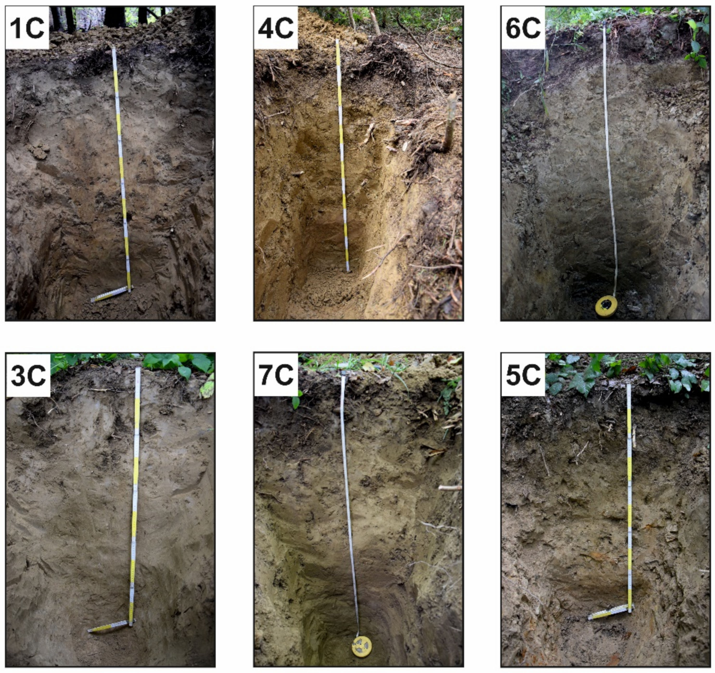
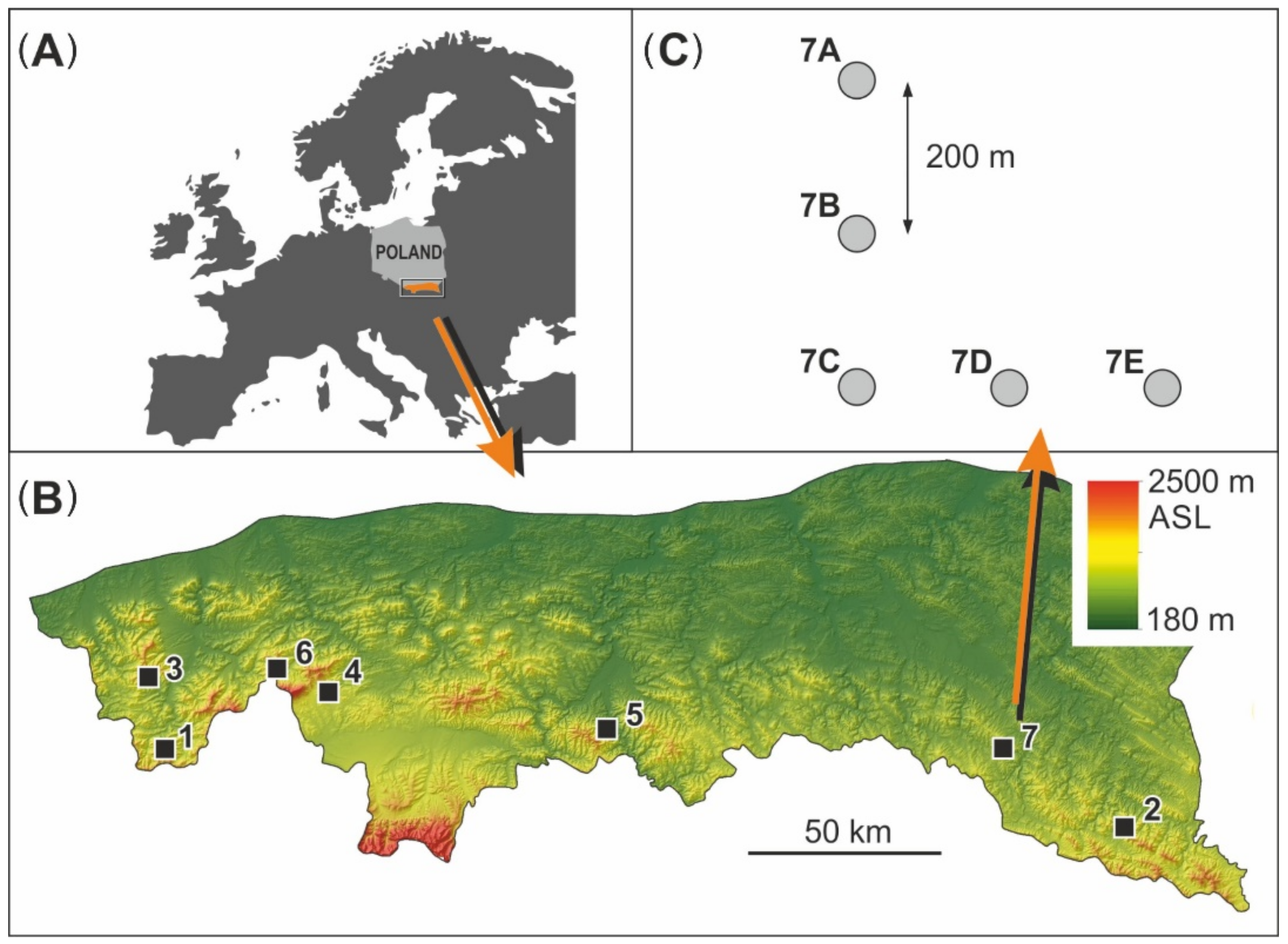
2.1. Study Area and Study Plot Selection
2.2. Field Survey
2.3. Sample Pretreatment, Laboratory Analysis and Soil Organic Matter Stock Estimation
2.4. Stand Characteristics and Coarse Root Biomass Estimation
2.5. Data Analysis
3. Results
3.1. Predictor Variances Among Beech-, Spruce- and Fir-Dominated Forests
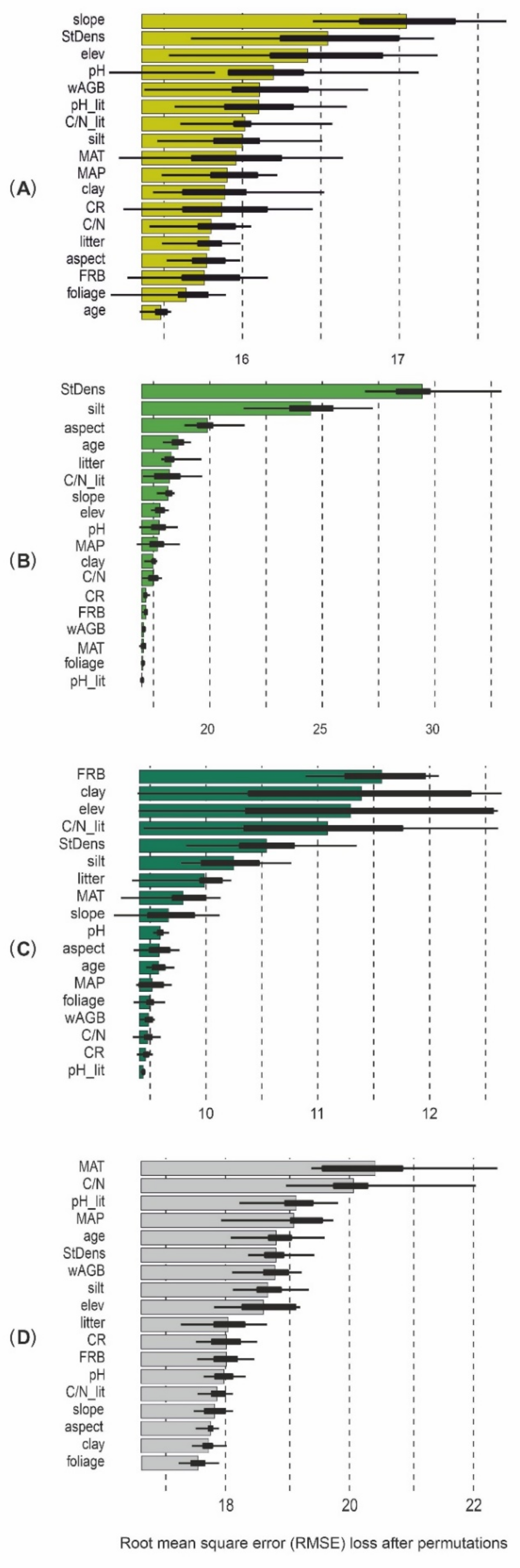
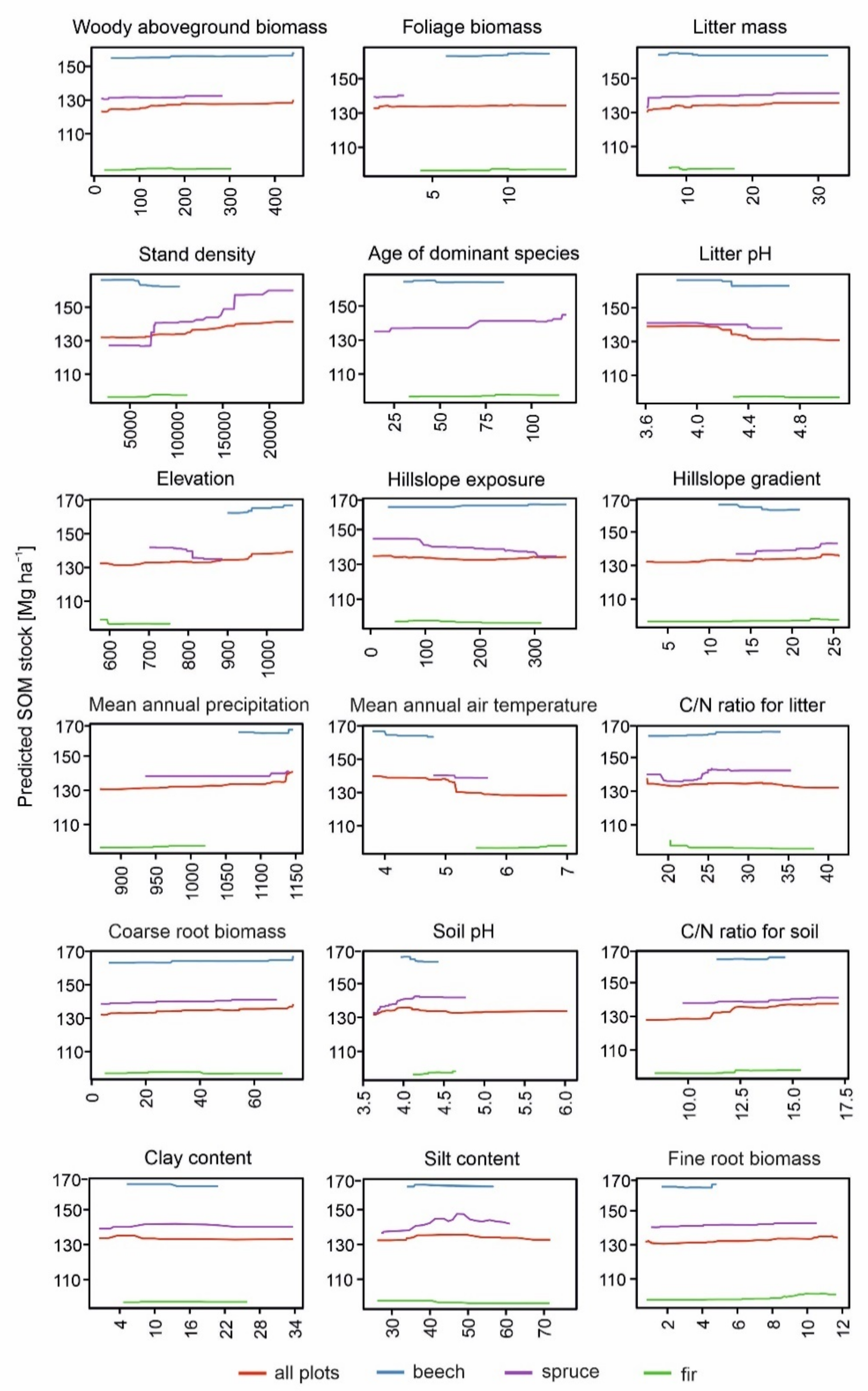
3.2. Determinants of Soil Organic Matter Stock and Fine Root Biomass in Beech-, Spruce- and Fir-Dominated Forests
4. Discussion
4.1. Relationships Between Selected Forest Characteristics and Fine Root Biomass
4.2. Relationships Between Selected Forest Characteristics and Soil Organic Matter Stock
4.3. Effect of Abiotic Factors on Fine Root Biomass and Soil Organic Matter Stock
5. Conclusions
Supplementary Materials
Author Contributions
Funding
Institutional Review Board Statement
Informed Consent Statement
Data Availability Statement
Acknowledgments
Conflicts of Interest
Appendix A

| Spruce | Beech | Fir | |||||||||||||
|---|---|---|---|---|---|---|---|---|---|---|---|---|---|---|---|
| Predictor * | Mean | Min | Max | Q1 | Q3 | Mean | Min | Max | Q1 | Q3 | Mean | Min | Max | Q1 | Q3 |
| age | 73.33 | 14.00 | 119.00 | 39.25 | 100.50 | 58.75 | 30.00 | 85.00 | 51.25 | 66.25 | 72.00 | 33.00 | 115.00 | 52.50 | 88.00 |
| StDens | 10247.81 | 2718.02 | 22580.58 | 6904.53 | 13841.36 | 6857.18 | 1854.14 | 10309.53 | 5023.46 | 9596.20 | 7418.84 | 2589.52 | 11191.39 | 4810.29 | 9736.49 |
| foliage | 2.06 | 1.07 | 3.10 | 1.48 | 2.48 | 9.89 | 5.90 | 12.84 | 8.73 | 11.83 | 9.69 | 4.20 | 13.90 | 8.79 | 11.18 |
| AGB | 114.93 | 15.53 | 284.07 | 35.42 | 161.34 | 220.34 | 36.81 | 441.70 | 109.06 | 360.15 | 156.14 | 21.82 | 303.42 | 91.60 | 225.74 |
| litter | 17.36 | 4.02 | 33.20 | 13.64 | 22.54 | 12.82 | 5.71 | 31.51 | 8.99 | 12.81 | 10.54 | 7.27 | 17.25 | 8.88 | 10.52 |
| C/N_lit | 24.90 | 17.32 | 35.27 | 21.48 | 26.76 | 26.40 | 17.51 | 33.96 | 22.60 | 31.36 | 27.75 | 20.24 | 38.21 | 22.56 | 32.66 |
| pH_lit | 4.27 | 3.61 | 4.66 | 4.16 | 4.40 | 4.26 | 3.84 | 4.72 | 4.22 | 4.28 | 4.62 | 4.28 | 5.11 | 4.39 | 4.76 |
| CR | 27.75 | 3.30 | 68.42 | 7.54 | 39.39 | 37.69 | 6.31 | 74.47 | 18.90 | 61.16 | 36.03 | 4.82 | 70.53 | 20.80 | 52.28 |
| FRB | 3.41 | 0.01 | 10.22 | 1.55 | 3.91 | 3.24 | 1.22 | 5.47 | 2.50 | 4.09 | 6.48 | 1.22 | 13.80 | 2.30 | 11.02 |
| SOM | 140.86 | 56.62 | 224.51 | 124.20 | 162.61 | 162.93 | 128.54 | 213.26 | 147.60 | 170.13 | 95.55 | 78.60 | 143.33 | 79.32 | 97.59 |
| C/N | 13.89 | 9.73 | 17.20 | 12.34 | 16.09 | 12.76 | 11.36 | 14.65 | 12.43 | 13.08 | 11.87 | 8.40 | 15.40 | 10.78 | 12.91 |
| pH | 4.08 | 3.62 | 4.77 | 3.82 | 4.19 | 4.18 | 3.96 | 4.43 | 4.06 | 4.31 | 4.39 | 4.11 | 4.64 | 4.24 | 4.61 |
| aspect | 193.92 | 4.37 | 340.16 | 113.48 | 281.15 | 273.25 | 31.97 | 358.52 | 276.88 | 317.71 | 139.14 | 44.60 | 312.47 | 67.85 | 200.94 |
| slope | 19.97 | 13.17 | 25.53 | 17.32 | 22.54 | 17.18 | 11.10 | 20.87 | 15.74 | 19.09 | 14.58 | 2.45 | 25.75 | 6.62 | 22.13 |
| elevation | 778.10 | 701.14 | 887.25 | 720.83 | 818.29 | 963.18 | 899.51 | 1066.85 | 932.67 | 978.80 | 654.12 | 575.64 | 753.32 | 614.76 | 701.89 |
| MAP | 1106.00 | 935.00 | 1140.00 | 1103.00 | 1131.00 | 1108.25 | 1068.00 | 1146.00 | 1068.00 | 1134.00 | 942.00 | 870.00 | 1021.00 | 904.50 | 968.00 |
| MAT | 5.14 | 4.78 | 5.74 | 4.99 | 5.23 | 4.51 | 3.81 | 4.78 | 4.49 | 4.78 | 6.25 | 5.54 | 6.97 | 5.91 | 6.64 |
| clay | 5.25 | 32.75 | 10.79 | 6.75 | 11.38 | 4.75 | 19.75 | 9.47 | 6.69 | 11.06 | 5.25 | 25.00 | 13.46 | 7.00 | 17.38 |
| silt | 28.00 | 59.25 | 40.33 | 32.69 | 45.75 | 35.75 | 64.25 | 48.41 | 44.06 | 51.69 | 26.50 | 71.00 | 49.82 | 38.88 | 60.25 |
References
- Nave, L.E.; Domke, G.M.; Hofmeister, K.L.; Mishra, U.; Perry, C.H.; Walters, B.F.; Swanston, C.W. Reforestation can sequester Table. Proc. Natl. Acad. Sci. USA 2018, 115, 2776–2781. [Google Scholar] [CrossRef] [Green Version]
- Pan, Y.; Birdsey, R.A.; Fang, J.; Houghton, R.; Kauppi, P.E.; Kurz, W.A.; Phillips, O.L.; Shvidenko, A.; Lewis, S.L.; Canadell, J.G.; et al. A large and persistent carbon sink in the world’s forests. Science 2011, 333, 988–993. [Google Scholar] [CrossRef] [Green Version]
- Dixon, R.K.; Brown, S.; Houghton, R.A.; Solomon, A.M.; Trexler, M.C.; Wisniewski, J. Carbon pools and flux of global forest ecosystems. Science 1994, 263, 185–190. [Google Scholar] [CrossRef] [PubMed]
- Lal, R. Soil Carbon Sequestration Impacts on Global Climate Change and Food Security. Science 2004, 304, 1623–1627. [Google Scholar] [CrossRef] [Green Version]
- Bojko, O.; Kabala, C. Organic carbon pools in mountain soils—Sources of variability and predicted changes in relation to climate and land use changes. Catena 2017, 149, 209–220. [Google Scholar] [CrossRef]
- Dieleman, W.I.J.; Venter, M.; Ramachandra, A.; Krockenberger, A.K.; Bird, M.I. Soil carbon stocks vary predictably with altitude in tropical forests: Implications for soil carbon storage. Geoderma 2013, 204, 59–67. [Google Scholar] [CrossRef]
- Liu, S.; Zhang, Z.B.; Li, D.M.; Hallett, P.D.; Zhang, G.L.; Peng, X.H. Temporal dynamics and vertical distribution of newly-derived carbon from a C3/C4 conversion in an Ultisol after 30-yr fertilization. Geoderma 2019, 337, 1077–1085. [Google Scholar] [CrossRef]
- Schepaschenko, D.; Moltchanova, E.; Shvidenko, A.; Blyshchyk, V.; Dmitriev, E.; Martynenko, O.; See, L.; Kraxner, F. Improved Estimates of Biomass Expansion Factors for Russian Forests. Forests 2018, 9, 312. [Google Scholar] [CrossRef] [Green Version]
- Vesterdal, L.; Clarke, N.; Sigurdsson, B.D.; Gundersen, P. Do tree species influence soil carbon stocks in temperate and boreal forests? For. Ecol. Manag. 2013, 309, 4–18. [Google Scholar] [CrossRef]
- Wasak, K.; Drewnik, M. Land use effects on soil organic carbon sequestration in calcareous Leptosols in former pastureland-a case study from the Tatra Mountains (Poland). Solid Earth 2015, 6, 1103–1115. [Google Scholar] [CrossRef] [Green Version]
- Baritz, R.; Seufert, G.; Montanarella, L.; Van Ranst, E. Carbon concentrations and stocks in forest soils of Europe. For. Ecol. Manag. 2010, 260, 262–277. [Google Scholar] [CrossRef]
- De Vos, B.; Cools, N.; Ilvesniemi, H.; Vesterdal, L.; Vanguelova, E.; Carnicelli, S. Benchmark values for forest soil carbon stocks in Europe: Results from a large scale forest soil survey. Geoderma 2015, 251, 33–46. [Google Scholar] [CrossRef]
- Jandl, R.; Lindner, M.; Vesterdal, L.; Bauwens, B.; Baritz, R.; Hagedorn, F.; Johnson, D.W.; Minkkinen, K.; Byrne, K.A. How strongly can forest management influence soil carbon sequestration? Geoderma 2007, 137, 253–268. [Google Scholar] [CrossRef]
- Lehtonen, A.; Palviainen, M.; Ojanen, P.; Kalliokoski, T.; Nöjd, P.; Kukkola, M.; Penttilä, T.; Mäkipää, R.; Leppälammi-Kujansuu, J.; Helmisaari, H.-S. Modelling fine root biomass of boreal tree stands using site and stand variables. For. Ecol. Manag. 2016, 359, 361–369. [Google Scholar] [CrossRef]
- Hobbie, S.E.; Ogdahl, M.; Chorover, J.; Chadwick, O.; Oleksyn, J.; Zytkowiak, R.; Reich, P. Tree Species Effects on Soil Organic Matter Dynamics: The Role of Soil Cation Composition. Ecosystems 2007, 10, 999–1018. [Google Scholar] [CrossRef]
- Galka, B.; Labaz, B.; Bogacz, A.; Bojko, O.; Kabala, C. Conversion of Norway spruce forests will reduce organic carbon pools in the mountain soils of SW Poland. Geoderma 2014, 213, 287–295. [Google Scholar] [CrossRef]
- Gruba, P.; Socha, J.; Błońska, E.; Lasota, J. Effect of variable soil texture, metal saturation of soil organic matter (SOM) and tree species composition on spatial distribution of SOM in forest soils in Poland. Sci. Total Environ. 2015, 521, 90–100. [Google Scholar] [CrossRef] [PubMed]
- Konôpka, B. Differences in fine root traits between norway spruce (Picea abies [L.] Karst.) and european beech (Fagus sylvatica L.)—A case study in the Kysucké Beskydy Mts. J. For. Sci. 2009, 55, 556–566. [Google Scholar] [CrossRef] [Green Version]
- Mueller, K.; Eissenstat, D.; Hobbie, S.; Oleksyn, J.; Jagodzinski, A.; Reich, B.; Chadwick, O.; Chorover, J. Tree species effects on coupled cycles of carbon, nitrogen, and acidity in mineral soils at a common garden experiment. Biogeochemistry 2012, 111, 601–614. [Google Scholar] [CrossRef]
- Ransedokken, Y.; Asplund, J.; Ohlson, M.; Nybakken, L. Vertical distribution of soil carbon in boreal forest under European beech and Norway spruce. Eur. J. For. Res. 2019, 138, 353–361. [Google Scholar] [CrossRef]
- Jagodziński, A.M.; Dyderski, M.K.; Gęsikiewicz, K.; Horodecki, P.; Cysewska, A.; Wierczyńska, S.; Maciejczyk, K. How do tree stand parameters affect young Scots pine biomass?—Allometric equations and biomass conversion and expansion factors. For. Ecol. Manag. 2018, 409, 74–83. [Google Scholar] [CrossRef]
- Jones, I.L.; DeWalt, S.J.; Lopez, O.R.; Bunnefeld, L.; Pattison, Z.; Dent, D.H. Above- and belowground carbon stocks are decoupled in secondary tropical forests and are positively related to forest age and soil nutrients respectively. Sci. Total Environ. 2019, 697, 133987. [Google Scholar] [CrossRef]
- Baumann, M.; Gasparri, I.; Piquer-Rodríguez, M.; Gavier Pizarro, G.; Griffiths, P.; Hostert, P.; Kuemmerle, T. Carbon emissions from agricultural expansion and intensification in the Chaco. Glob. Chang. Biol. 2017, 23, 1902–1916. [Google Scholar] [CrossRef]
- Erb, K.H.; Kastner, T.; Plutzar, C.; Bais, A.L.S.; Carvalhais, N.; Fetzel, T.; Gingrich, S.; Haberl, H.; Lauk, C.; Niedertscheider, M.; et al. Unexpectedly large impact of forest management and grazing on global vegetation biomass. Nature 2018, 553, 73–76. [Google Scholar] [CrossRef] [PubMed]
- Hansen, M.C. High-Resolution Global Maps of Journal. Science 2013, 850, 850–854. [Google Scholar] [CrossRef] [Green Version]
- Tyukavina, A.; Baccini, A.; Hansen, M.C.; Potapov, P.V.; Stehman, S.V.; Houghton, R.A.; Krylov, A.M.; Turubanova, S.; Goetz, S.J. Aboveground carbon loss in natural and managed tropical forests from 2000 to 2012. Environ. Res. Lett. 2015, 10, 74002. [Google Scholar] [CrossRef]
- Forrester, D.I.; Tachauer, I.H.H.; Annighoefer, P.; Barbeito, I.; Pretzsch, H.; Ruiz-Peinado, R.; Stark, H.; Vacchiano, G.; Zlatanov, T.; Chakraborty, T.; et al. Generalized biomass and leaf area allometric equations for European tree species incorporating stand structure, tree age and climate. For. Ecol. Manag. 2017, 396, 160–175. [Google Scholar] [CrossRef]
- Duncanson, L.; Armston, J.; Disney, M.; Avitabile, V.; Barbier, N.; Calders, K.; Carter, S.; Chave, J.; Herold, M.; Crowther, T.W.; et al. The Importance of Consistent Global Forest Aboveground Biomass Product Validation. Surv. Geophys. 2019, 40, 979–999. [Google Scholar] [CrossRef] [Green Version]
- Matasci, G.; Hermosilla, T.; Wulder, M.A.; White, J.C.; Coops, N.C.; Hobart, G.W.; Zald, H.S.J. Large-area mapping of Canadian boreal forest cover, height, biomass and other structural attributes using Landsat composites and lidar plots. Remote Sens. Environ. 2018, 209, 90–106. [Google Scholar] [CrossRef]
- Schwieder, M.; Leitão, P.J.; Pinto, J.R.R.; Teixeira, A.M.C.; Pedroni, F.; Sanchez, M.; Bustamante, M.M.; Hostert, P. Landsat phenological metrics and their relation to aboveground carbon in the Brazilian Savanna. Carbon Balance Manag. 2018, 13, 7. [Google Scholar] [CrossRef] [Green Version]
- Wulder, M.A.; White, J.C.; Nelson, R.F.; Næsset, E.; Ørka, H.O.; Coops, N.C.; Hilker, T.; Bater, C.W.; Gobakken, T. Lidar sampling for large-area forest characterization: A review. Remote Sens. Environ. 2012, 121, 196–209. [Google Scholar] [CrossRef] [Green Version]
- Don, A.; Schumacher, J.; Scherer-Lorenzen, M.; Scholten, T.; Schulze, E.D. Spatial and vertical variation of soil carbon at two grassland sites—Implications for measuring soil carbon stocks. Geoderma 2007, 141, 272–282. [Google Scholar] [CrossRef]
- Leifeld, J.; Kögel-Knabner, I. Soil organic matter fractions as early indicators for carbon stock changes under different land-use? Geoderma 2005, 124, 143–155. [Google Scholar] [CrossRef]
- Matamala, R.; Gonzàlez-Meler, M.A.; Jastrow, J.D.; Norby, R.J.; Schlesinger, W.H. Impacts of fine root turnover on forest NPP and soil C sequestration potential. Science 2003, 302, 1385–1387. [Google Scholar] [CrossRef] [PubMed]
- Finér, L.; Helmisaari, H.S.; Lõhmus, K.; Majdi, H.; Brunner, I.; Børja, I.; Eldhuset, T.; Godbold, D.; Grebenc, T.; Konôpka, B.; et al. Variation in fine root biomass of three European tree species: Beech (Fagus sylvatica L.), Norway spruce (Picea abies L. Karst.), and Scots pine (Pinus sylvestris L.). Plant Biosyst. 2007, 141, 394–405. [Google Scholar] [CrossRef]
- Silver, W.L.; Miya, R.K. Global patterns in root decomposition: Comparisons of climate and litter quality effects. Oecologia 2001, 129, 407–419. [Google Scholar] [CrossRef]
- Don, A.; Scholten, T.; Schulze, E.D. Conversion of cropland into grassland: Implications for soil organic-carbon stocks in two soils with different texture. J. Plant Nutr. Soil Sci. 2009, 172, 53–62. [Google Scholar] [CrossRef]
- Leuschner, C.; Backes, K.; Hertel, D.; Schipka, F.; Schmitt, U.; Terborg, O.; Runge, M. Drought responses at leaf, stem and fine root levels of competitive Fagus sylvatica L. and Quercus petraea (Matt.) Liebl. trees in dry and wet years. For. Ecol. Manag. 2001, 149, 33–46. [Google Scholar] [CrossRef]
- Persson, H. The distribution and productivity of fine roots in boreal forests. Plant Soil. 1983, 71, 87–101. [Google Scholar] [CrossRef]
- Finzi, A.C.; Abramoff, R.Z.; Spiller, K.S.; Brzostek, E.R.; Darby, B.A.; Kramer, M.A.; Phillips, R.P. Rhizosphere processes are quantitatively important components of terrestrial carbon and nutrient cycles. Glob. Chang. Biol. 2015, 21, 2082–2094. [Google Scholar] [CrossRef]
- Han, M.; Sun, L.; Gan, D.; Fu, L.; Zhu, B. Root functional traits are key determinants of the rhizosphere effect on soil organic matter decomposition across 14 temperate hardwood species. Soil Biol. Biochem. 2020, 151, 108019. [Google Scholar] [CrossRef]
- Sun, L.; Ataka, M.; Kominami, Y.; Yoshimura, K. Relationship between fine-root exudation and respiration of two Quercus species in a Japanese temperate forest. Tree Physiol. 2017, 37, 1011–1020. [Google Scholar] [CrossRef]
- Mao, R.; Zeng, D.H.; Li, L. Fresh root decomposition pattern of two contrasting tree species from temperate agroforestry systems: Effects of root diameter and nitrogen enrichment of soil. Plant Soil. 2011, 347, 115–123. [Google Scholar] [CrossRef]
- Zhang, X.; Wang, W. The decomposition of fine and coarse roots: Their global patterns and controlling factors. Sci. Rep. 2015, 5. [Google Scholar] [CrossRef] [PubMed]
- Clemmensen, K.E.; Bahr, A.; Ovaskainen, O.; Dahlberg, A.; Ekblad, A.; Wallander, H.; Stenlid, J.; Finlay, R.D.; Wardle, D.A.; Lindahl, B.D. Roots and associated fungi drive long-term carbon sequestration in boreal forest. Science 2013, 340, 1615–1618. [Google Scholar] [CrossRef]
- Raich, J.W.; Clark, D.A.; Schwendenmann, L.; Wood, T.E. Aboveground tree growth varies with belowground carbon allocation in a tropical rainforest environment. PLoS ONE 2014, 9, e100275. [Google Scholar] [CrossRef] [PubMed] [Green Version]
- Rasse, D.P.; Rumpel, C.; Dignac, M.F. Is soil carbon mostly root carbon? Mechanisms for a specific stabilisation. Plant Soil 2005, 269, 341–356. [Google Scholar] [CrossRef]
- Kozłowski, T.T.; Pallardy, S.G. Physiology of Woody Plants; Academic Press: San Diego, CA, USA, 1997. [Google Scholar]
- Canarini, A.; Kaiser, C.; Merchant, A.; Richter, A.; Wanek, W. Root Exudation of Primary Metabolites: Mechanisms and Their Roles in Plant Responses to Environmental Stimuli. Front. Plant Sci. 2019, 10, 157. [Google Scholar] [CrossRef] [Green Version]
- McCormack, M.L.; Dickie, I.A.; Eissenstat, D.M.; Fahey, T.J.; Fernandez, C.W.; Guo, D.; Helmisaari, H.S.; Hobbie, E.A.; Iversen, C.M.; Jackson, R.B.; et al. Redefining fine roots improves understanding of below-ground contributions to terrestrial biosphere processes. New Phytol. 2015, 207, 505–518. [Google Scholar] [CrossRef]
- Franklin, J.; Serra-Diaz, J.M.; Syphard, A.D.; Regan, H.M. Global change and terrestrial plant community dynamics. Proc. Natl. Acad. Sci. USA 2016, 113, 3725–3734. [Google Scholar] [CrossRef] [Green Version]
- Wang, X.; Tang, C.; Severi, J.; Butterly, C.R.; Baldock, J.A. Rhizosphere priming effect on soil organic carbon decomposition under plant species differing in soil acidification and root exudation. New Phytol. 2016, 211, 864–873. [Google Scholar] [CrossRef]
- Błońska, E.; Lasota, J.; Gruba, P. Effect of temperate forest tree species on soil dehydrogenase and urease activities in relation to other properties of soil derived from loess and glaciofluvial sand. Ecological. Res. 2016, 31, 655–664. [Google Scholar] [CrossRef] [Green Version]
- Horodecki, P.; Nowiński, M.; Jagodziński, A.M. Advantages of mixed tree stands in restoration of upper soil layers on postmining sites: A five-year leaf liter decomposition experiment. Land Degrad. Dev. 2019, 30, 3–13. [Google Scholar] [CrossRef] [Green Version]
- Sjöström, E.; Westermark, U. Chemical composition of wood and pulps: Basic constituents and their distribution. In Analytical Methods in Wood Chemistry, Pulping, and Papermaking; Sjöström, E., Alén, R., Eds.; Springer: Berlin, Germany, 1999; pp. 1–19. [Google Scholar]
- Mayer, M.; Prescott, C.; Abaker, W.; Augusto, L.; Cécillon, L.; Ferreira, G.; James, J.; Jandl, R.; Katzensteiner, K.; Laclau, J.P.; et al. Influence of forest management activities on soil organic carbon stocks: A knowledge synthesis. For. Ecol. Manag. 2020, 466. [Google Scholar] [CrossRef]
- Schepaschenko, D.; Shvidenko, A.; Usoltsev, V.; Lakyda, P.; Luo, Y.; Vasylyshyn, R.; Lakyda, I.; Myklush, Y.; See, L.; McCallum, I.; et al. A dataset of forest biomass structure for Eurasia. Sci. Data 2017, 4, sdata201770. [Google Scholar] [CrossRef] [PubMed]
- Dyderski, M.K.; Pawlik, Ł. Spatial distribution of tree species in mountain national parks depends on geomorphology and climate. For. Ecol. Manag. 2020, 474, 118366. [Google Scholar] [CrossRef]
- Wypych, A.; Ustrnul, Z.; Schmatz, D.R. Long-term variability of air temperature and precipitation conditions in the Polish Carpathians. J. Mt. Sci. 2018, 15, 237–253. [Google Scholar] [CrossRef]
- Grabska, E.; Hostert, P.; Pflugmacher, D.; Ostapowicz, K. Forest stand species mapping using the sentinel-2 time series. Remote Sens. 2019, 11, 1197. [Google Scholar] [CrossRef] [Green Version]
- Matiakowska, J.; Szabla, K. Beskidy bez lasu? Magazyn Społeczno-Kulturalny “Śląsk”; Górnośląskie Towarzystwo Literackie: Katowice, Poland, 2007. [Google Scholar]
- Turnock, D. Ecoregion-based conservation in the Carpathians and the land-use implications. Land Use Pol. 2002, 19, 47–63. [Google Scholar] [CrossRef]
- Kacprzak, A.; Szymański, W.; Wojcik-Tabol, P. The role of flysch sandstones in forming the properties of cover deposits and soils—Examples from the Carpathians. Z. Geomorphol. 2015, 59. [Google Scholar] [CrossRef]
- Skiba, S.; Drewnik, M. Mapa gleb obszaru Karpat w granicach Polski. Rocz. Bieszcz. 2003, 11, 15–20. [Google Scholar]
- FAO. Guidelines for Soil Description, 4th ed.; Food and Agriculture Organization of the United Nations (FAO): Rome, Italy, 2006. [Google Scholar]
- IUSS Working Group WRB. World Reference Base for Soil Resources 2014. International Soil Classification System for Naming Soils and Creating Legends for Soil Maps; World Soil Resources Reports No. 106; FAO: Rome, Italy, 2014; Update 2015. [Google Scholar]
- Anderson, L.J.; Comas, L.H.; Lakso, A.N.; Eissenstat, D.M. Multiple risk factors in root survivorship: A four-year study in Concord grape. New Phytol. 2003, 158, 489–501. [Google Scholar] [CrossRef] [Green Version]
- Eissenstat, D.M.; Yanai, R.D. The ecology of root lifespan. Adv. Ecol. Res. 1997, 27, 1–60. [Google Scholar] [CrossRef]
- Thomas, G.W. Soil pH and Soil Acidity. In Methods of Soil Analysis. Part 3, Chemical Methods; Sparks, D.L., Page, A.L., Helmke, P.A., Loeppert, R.H., Eds.; SSSA and ASA: Madison, WI, USA, 1996; pp. 475–490. [Google Scholar]
- Egli, M.; Sartori, G.; Mirabella, A.; Giaccai, D. The effects of exposure and climate on the weathering of late Pleistocene and Holocene Alpine soils. Geomorphology 2010, 114, 466–482. [Google Scholar] [CrossRef] [Green Version]
- Gee, G.W.; Bauder, J.W. Particle-Size Analysis. In Methods of Soil Analysis. Part 1, Physical and Mineralogical Methods; Klute, A., Ed.; ASA-SSSA: Madison, WI, USA, 1986; pp. 427–445. [Google Scholar]
- Pribyl, D. A critical review of conventional SOC to SOM conversion factor. Geoderma 2010, 156, 75–83. [Google Scholar] [CrossRef]
- Jagodziński, A.M.; Dyderski, M.K.; Horodecki, P. Differences in biomass production and carbon sequestration between highland and lowland stands of Picea abies (L.) H. Karst. and Fagus sylvatica L. For. Ecol. Manag. 2020, 474, 118329. [Google Scholar] [CrossRef]
- Jagodziński, A.M.; Dyderski, M.K.; Gęsikiewicz, K.; Horodecki, P. Tree and stand level estimations of Abies alba Mill. aboveground biomass. Ann. For. Sci. 2019, 76, 56. [Google Scholar] [CrossRef] [Green Version]
- Biecek, P. DALEX: Explainers for Complex Predictive Models in R. J. Mach. Learn. Res. 2018, 19, 84. [Google Scholar]
- Breiman, L. Random forests. Mach. Learn 2001, 45, 5–32. [Google Scholar] [CrossRef] [Green Version]
- Hengl, T.; Walsh, M.G.; Sanderman, J.; Wheeler, I.; Harrison, S.P.; Prentice, I.C. Global mapping of potential natural vegetation: An assessment of machine learning algorithms for estimating land potential. PeerJ 2018, 6, e5457. [Google Scholar] [CrossRef] [Green Version]
- R Core Team. R: A Language and Environment for Statistical Computing; R Foundation for Statistical Computing: Vienna, Austria, 2016. [Google Scholar]
- Kuhn, M. Building Predictive Models in R Using the caret Package. J. Stat. Soft. 2008, 28, 1–26. [Google Scholar] [CrossRef] [Green Version]
- Addo-Danso, S.D.; Prescott, C.E.; Smith, A.R. Methods for estimating root biomass and production in forest and woodland ecosystem carbon studies: A review. For. Ecol. Manag. 2016, 359, 332–351. [Google Scholar] [CrossRef]
- Jurasinski, G.; Jordan, A.; Glatzel, S. Mapping soil CO2 efflux in an old-growth forest using regression kriging with estimated fine root biomass as ancillary data. For. Ecol. Manag. 2012, 263, 101–113. [Google Scholar] [CrossRef]
- Mooney, H.A.; Chu, C. Seasonal carbon allocation in Heteromeles arbutifolium, a California evergreen shrub. Oecologia 1974, 14, 295–306. [Google Scholar] [CrossRef]
- Helmisaari, H.; Derome, J.; Nöjd, P.; Kukkola, M. Fine root biomass in relation to site and stand characteristics in Norway spruce and Scots pine stands. Tree Physiol. 2007, 27, 1493–1504. [Google Scholar] [CrossRef] [Green Version]
- Chen, W.; Zhang, Q.; Cihlar, J.; Bauhus, J.; Price, D.T. Estimating fine-root biomass and production of boreal and cool temperate forests using aboveground measurements: A new approach. Plant Soil 2004, 265, 31–46. [Google Scholar] [CrossRef]
- Kirfel, K.; Heinze, S.; Hertel, D.; Leuschner, C. Effects of bedrock type and soil chemistry on the fine roots of European beech—A study on the belowground plasticity of trees. For. Ecol. Manag. 2019, 444, 256–268. [Google Scholar] [CrossRef]
- Jagodziński, A.M.; Ziółkowski, J.; Warnkowska, A.; Prais, H. Tree Age Effects on Fine Root Biomass and Morphology over Chronosequences of Fagus sylvatica, Quercus robur and Alnus glutinosa Stands. PLoS ONE 2016, 11, e0148668. [Google Scholar] [CrossRef]
- Jobbagy, E.G.; Jackson, R.B. The vertical distribution of soil organic carbon and its relation to climate and vegetation. Ecol. Appl. 2000, 10, 423–436. [Google Scholar] [CrossRef]
- Vogt, K.A.; Vogt, D.J.; Palmiotto, P.A.; Boon, P.; O’Hara, J.; Asbjornsen, H. Review of root dynamics in forest ecosystems grouped by climate, climatic forest type and species. Plant Soil 1995, 187, 159–219. [Google Scholar] [CrossRef]
- Leuschner, C.; Ellenberg, H. Ecology of Central European Forests: Vegetation Ecology of Central Europe, Volume I; Springer: Cham, Switzerland, 2017. [Google Scholar]
- Schenk, H.J.; Jackson, R.B. The global biogeography of roots. Ecol. Monogr. 2002, 72, 311–328. [Google Scholar] [CrossRef]
- Leifeld, J.; Zimmerman, M.; Fuhrer, J.; Conen, F. Storage and turnover of carbon in grassland soils along an elevation gradiend in the Swiss Alps. Glob. Chang. Biol. 2009, 15, 668–679. [Google Scholar] [CrossRef]
- Makkonen, K.; Helmisaari, H. Assessing fine-root biomass and production in a Scots pine stand—Comparison of soil core and root ingrowth core methods. Plant Soil 1999, 210, 43–50. [Google Scholar] [CrossRef]
- Yuan, Z.Y.; Chen, H.Y.H. Indirect Methods Produce Higher Estimates of Fine Root Production and Turnover Rates than Direct Methods. PLoS ONE 2012, 7, e48989. [Google Scholar] [CrossRef]
- Day, F.P.; Schroeder, R.E.; Stover, D.B.; Brown, A.L.P.; Butnor, J.R.; Dilustro, J.; Hungate, B.A.; Dijkstra, P.; Duval, B.D.; Seiler, T.J.; et al. The effects of 11 yr of CO2 enrichment on roots in a Florida scrub-oak ecosystem. New Phytol. 2013, 200, 778–787. [Google Scholar] [CrossRef] [PubMed] [Green Version]
- Augusto, L.; Dupouey, J.L.; Ranger, J. Effects of tree species on understory vegetation and environmental conditions in temperate forests. Ann. For. Sci. 2003, 60, 823–831. [Google Scholar] [CrossRef]
- Gurmesa, G.A.; Schmidt, I.K.; Gundersen, P.; Vesterdal, L. Soil carbon accumulation and nitrogen retention traits of four tree species grown in common gardens. For. Ecol. Manag. 2013, 309, 47–57. [Google Scholar] [CrossRef]
- Cremer, M.; Kern, N.V.; Prietzel, J. Soil organic carbon and nitrogen stocks under pure and mixed stands of European beech, Douglas fir and Norway spruce. For. Ecol. Manag. 2017, 367, 30–40. [Google Scholar] [CrossRef]
- Angst, G.; Mueller, K.; Eissenstat, D.; Trumbore, S.; Freeman, K.; Hobbie, S.; Chorover, J.; Oleksyn, J.; Reich, P.; Mueller, C. Soil organic carbon stability in forests: Distinct effects of tree species identity and traits. Glob. Chang. Biol. 2019, 25, 1529–1546. [Google Scholar] [CrossRef]
- Kögel-Knabner, I.; Guggenberger, G.; Kleber, M.; Kandeler, M.; Kalbitz, K.; Scheu, S.; Eusterhues, K.; Leinweber, P. Organo-mineral associations in temperate soils: Integrating biology, mineralogy, and organic matter chemistry. J. Plant Nutr. Soil Sci. 2008, 171, 61–82. [Google Scholar] [CrossRef]
- Lützow, M.V.; Kögel-Knabner, I.; Ekschmitt, K.; Matzner, E.; Guggenberger, G.; Marschner, B.; Flessa, H. Stabilization of organic matter in temperate soils: Mechanisms and their rele- vance under different soil conditions—A review. Eur. J. Soil Sci. 2006, 57, 426–445. [Google Scholar] [CrossRef]
- Lei, P.; Scherer-Lorenzen, M.; Bauhus, J. Belowground facilitation and competition in young tree species mixtures. For. Ecol. Manag. 2012, 265, 191–200. [Google Scholar] [CrossRef]
- Yimer, F.; Ledin, S.; Abdelkadir, A. Soil organic carbon and total nitrogen stocks as affected by topographic aspect and vegetation in the Bale Mountains, Ethiopia. Geoderma 2006, 135, 335–344. [Google Scholar] [CrossRef]
- Matos, E.S.; Freese, D.; Ślazak, A.; Bachmann, U.; Veste, M.; Hüttl, R.F. Organic-carbon and nitrogen stocks and organic-carbon fractions in soil under mixed pine and oak forest stands of different ages in NE Germany. J. Plant Nutr. Soil Sci. 2010, 173, 654–661. [Google Scholar] [CrossRef]
- Targulian, V.O.; Krasilnikov, P.V. Soil system and pedogenic processes: Self-organization, time scales, and environmental significance. Catena 2007, 71, 373–381. [Google Scholar] [CrossRef]
- Gaul, D.; Hertel, D.; Leuschner, C. Effects of experimental soil frost on the fine-root system of mature Norway spruce. J Plant Nutr. Soil Sci. 2008, 171, 690–698. [Google Scholar] [CrossRef]
- Leuschner, C.; Hertel, D.; Schmid, I.; Koch, O.; Muhs, A.; Holscher, D. Stand fine root biomass and fine root morphology in old- growth beech forests as a function of precipitation and soil fertility. Plant Soil 2004, 258, 43–56. [Google Scholar] [CrossRef]
- Norby, R.J.; Jackson, R.B. Root dynamics and global change: Seeking an ecosystem perspective. New Phytol. 2000, 147, 3–12. [Google Scholar] [CrossRef] [Green Version]
- Yuan, Z.Y.; Chen, H.Y.H. Fine Root Biomass, Production, Turnover Rates, and Nutrient Contents in Boreal Forest Ecosystems in Relation to Species, Climate, Fertility, and Stand Age: Literature Review and Meta-Analyses. Crit. Rev. Plant Sci. 2010, 29, 204–221. [Google Scholar] [CrossRef]
- Britton, A.J.; Helliwell, R.C.; Lilly, A.; Dawson, L.; Fisher, J.M.; Coull, M.; Ross, J. An integrated assessment of ecosystem carbon pools and fluxes across an oceanic alpine toposequence. Plant Soil 2011, 345, 287–302. [Google Scholar] [CrossRef]
- Djukic, I.; Zehetner, F.; Tatzber, M.; Gerzabek, M.H. Soil organic-matter stocks and characteristics along an alpine elevation gradient. J. Plant Nut. Soil Sci. 2010, 173, 30–38. [Google Scholar] [CrossRef]
- Drewnik, M. The effect of environmental conditions on the decomposition rate of cellulose in mountain soils. Geoderma 2006, 132, 116–130. [Google Scholar] [CrossRef]
- Hobbie, S.E.; Reich, P.B.; Oleksyn, J.; Ogdahl, M.; Zytkowiak, R.; Hale, C.; Karolewski, P. Tree species effects on decomposition and forest floor dynamics in a common garden. Ecology 2006, 87, 2288–2297. [Google Scholar] [CrossRef]
- Klimek, B.; Niklińska, M.; Jaźwa, M.; Tarasek, A.; Tekielak, I.; Musielok, Ł. Covariation of soil bacteria functional diversity and vegetation diversity along an altitudinal climatic gradient in the Western Carpathians. Pedobiologia 2015, 58, 105–112. [Google Scholar] [CrossRef]
- Niklińska, M.; Klimek, B. Dynamics and stratification of soil biota activity along an altitudinal climatic gradient in West Carpathians. J. Biol. Res. 2011, 16, 177–187. [Google Scholar]
- Taten, R.; Takeda, H. Forest structure and tree species distribution in relation to topography-mediated heterogeneity of soil nitrogen and light at the forest floor. Ecol. Res. 2003, 18, 559–571. [Google Scholar] [CrossRef]
- Espleta, J.F.; Clark, D.A. Multi-scale variation in fine-root biomass in a tropical rain forest: A seven-year study. Ecol. Monogr. 2007, 77, 377–404. [Google Scholar] [CrossRef] [Green Version]
- Leifeld, J.; Bassin, S.; Conen, F.; Hajdas, I.; Egli, M.; Fuhrer, J. Control of soil pH on turnover of belowground organic matter in subalpine grassland. Biogeochemistry 2013, 112, 59–69. [Google Scholar] [CrossRef] [Green Version]
- Tan, Z.; Lal, R.; Smeck, N.E.; Calhoun, F.G.; Slater, B.K.; Parkinson, B.; Gehring, R.M. Taxonomic and geographic distribution of soil organic carbon pools in Ohio. Soil Sci. Soc. Am. J. 2004, 68, 1896–1904. [Google Scholar] [CrossRef]


| Study Site | Coordinates | Elevation Range Min–Max (m a.s.l.) | Hillslope Gradient Range Min–Max (°) | Hillslope Exposure Range Min–Max (°) | Mean Annual Air Temperature (°C) | Mean Annual Precipitation (mm) |
|---|---|---|---|---|---|---|
| 1 | 49°26′54″ N 19°03′05″ E | 701–808 | 13–24 | 4–165 | 5.1 | 1127 |
| 2 | 49°11′30″ N 22°28′12″ E | 940–1067 | 11–21 | 276–316 | 4.6 | 1068 |
| 3 | 49°38′01″ N 18°58′36″ E | 768–887 | 15–25 | 218–319 | 5.2 | 1103 |
| 4 | 49°34′28″ N 19°41′09″ E | 706–753 | 2–22 | 44–340 | 5.5 | 978 |
| 5 | 49°29′27″ N 20°36′35″ E | 575–658 | 21–26 | 59–79 | 6.3 | 1021 |
| 6 | 49°37′44″ N 19°28′30″ E | 836–937 | 16–20 | 32–358 | 4.8 | 1134 |
| 7 | 49°25′10″ N 22°01′56″ E | 602–624 | 8–16 | 100–266 | 6.1 | 870 |
| Abbreviation | Predictor | Unit |
|---|---|---|
| wAGB | Woody aboveground biomass | Mg ha−1 |
| StDens | Stand density | ind ha−1 |
| foliage | Foliage biomass | Mg ha−1 |
| age | Age of dominant species | years |
| litter | Litter mass | Mg ha−1 |
| pH_lit | Litter pH (in H2O) | dimensionless |
| C/N_lit | Organic Carbon/Nitrogen ratio in litter | dimensionless |
| MAT | Mean annual air temperature | °C |
| MAP | Mean annual precipitation | mm |
| elev | Elevation | m a.s.l. |
| slope | Hillslope gradient | ° |
| aspect | Hillslope exposure | ° |
| SOM * | Soil Organic Matter stock | Mg ha−1 |
| C/N * | Organic Carbon/Nitrogen ratio in soil | dimensionless |
| Clay * | Clay content | % |
| Silt * | Silt content | % |
| pH * | Soil pH (in H2O) | dimensionless |
| CR * | Coarse roots biomass | Mg ha−1 |
| FRB * | Fine roots biomass | Mg ha−1 |
| Study Plot | Woody Aboveground Biomass Stock (wAGB) | Plot Type * | Litter | C/N Litter Ratio | Time of Fieldwork | ||||
|---|---|---|---|---|---|---|---|---|---|
| Beech | Spruce | Fir | Other Species | Total | |||||
| Mg ha−1 | |||||||||
| 1A | 38.48 | 245.59 | - | - | 284.07 | spruce | 33.20 | 35 | 22 September 2017 |
| 1B | 1.30 | 211.54 | - | - | 212.84 | spruce | 16.05 | 17 | 22 September 2017 |
| 1C | - | 185.62 | - | 2.25 | 187.87 | spruce | 22.00 | 21 | 22 September2017 |
| 1D | - | 95.50 | - | - | 95.50 | spruce | 24.18 | 25 | 22 June 2017 |
| 1E | - | 118.75 | - | 33.75 | 152.50 | spruce | 25.46 | 26 | 22 June 2017 |
| 2A | 334.45 | - | - | - | 334.45 | beech | 12.73 | 34 | 7 July 2017 |
| 2B | 197.05 | - | - | - | 197.05 | beech | 10.86 | 32 | 7 July 2017 |
| 2C | 36.81 | - | - | - | 36.81 | beech | 31.51 | 25 | 7 July 2017 |
| 2D | 437.26 | - | - | - | 437.26 | beech | 13.03 | 31 | 7 July 2017 |
| 2E | 441.70 | - | - | - | 441.70 | beech | 8.54 | 27 | 7 July 2017 |
| 3A | - | 15.14 | 0.39 | - | 15.53 | spruce | 19.50 | 21 | 20 June 2017 |
| 3B | - | 25.55 | - | - | 25.55 | spruce | 4.02 | 29 | 20 June 2017 |
| 3C | 31.01 | 67.70 | 3.49 | - | 102.21 | spruce | 15.51 | 31 | 20 June 2017 |
| 3D | 12.82 | 90.49 | - | - | 103.31 | spruce | 17.90 | 22 | 20 June 2017 |
| 3E | 9.85 | 28.62 | 0.25 | - | 38.71 | spruce | 18.13 | 25 | 20 June 2017 |
| 4A | - | 104.93 | 40.29 | - | 145.23 | spruce | 8.04 | 22 | 28 August 2017 |
| 4B | - | 15.49 | 60.22 | 9.02 | 84.74 | fir | 10.46 | 36 | 28 August 2017 |
| 4C | - | 8.45 | 226.53 | - | 234.98 | fir | 10.58 | 20 | 28 August 2017 |
| 4E | - | 31.79 | 10.85 | 128.52 | 171.15 | other | 9.37 | 32 | 28 August 2017 |
| 5A | - | 2.29 | 130.77 | - | 133.06 | fir | 8.09 | 20 | 5 November 2017 |
| 5B | 2.88 | - | 18.95 | - | 21.82 | fir | 9.67 | 25 | 5 November 2017 |
| 5C | - | - | 98.47 | - | 98.47 | fir | 17.25 | 29 | 5 November 2017 |
| 6A | 21.09 | 2.54 | 25.53 | 8.90 | 58.06 | fir | 10.88 | 41 | 9 September 2017 |
| 6B | - | 15.79 | - | - | 15.79 | spruce | 13.53 | 23 | 9 September 2017 |
| 6C | 128.49 | - | - | - | 128.49 | beech | 9.14 | 23 | 9 September 2017 |
| 6D | 109.81 | - | 26.43 | - | 136.23 | beech | 11.04 | 22 | 9 September 2017 |
| 6E | 36.55 | 9.65 | 4.55 | - | 50.76 | beech | 5.71 | 18 | 9 September 2017 |
| 7A | - | 24.74 | 2.48 | 82.40 | 109.62 | other | 9.92 | 32 | 29 August 2017 |
| 7B | 13.53 | - | 202.98 | - | 216.50 | fir | 7.27 | 38 | 29 August 2017 |
| 7C | 9.67 | - | 10.49 | 28.41 | 48.57 | other | 9.37 | 32 | 29 August 2017 |
| 7D | - | - | 48.69 | 51.86 | 100.55 | other | 7.10 | 35 | 29 August 2017 |
| 7E | 7.76 | - | 281.96 | 13.69 | 303.42 | fir | 10.45 | 25 | 29 August 2017 |
| Species Composition (%) * | Forest Stand Parameters | Forest Management | ||||||
|---|---|---|---|---|---|---|---|---|
| Study Plot | Beech | Spruce | Fir | Others | Stand Density (ind ha−1) | Foliage (Mg ha−1) | Age of Dominant Species (Years) | Forest Cover or Species Composition Changes ** |
| 1A | 29.7 | 70.3 | - | - | 15,958.3 | 12.9 | 99 | NO (1933) |
| 1B | 3.7 | 92.6 | - | 3.7 | 22,580.6 | 11.7 | 119 | NO (1933) |
| 1C | - | 100 | - | - | 7605.3 | 11.2 | 114 | NO (1933) |
| 1D | 2.5 | 95.0 | - | 2.5 | 16495.2 | 9.0 | 99 | NO (1933) |
| 1E | 21.1 | 73.7 | - | 5.3 | 7835.2 | 10.3 | 99 | NO (1933) |
| 2A | 100 | - | - | - | 10,309.5 | 2.9 | 85 | NO (1937) |
| 2B | 100 | - | - | - | 5291.2 | 2.4 | 60 | NO (1937) |
| 2C | 100 | - | - | - | 1854.1 | 1.2 | 60 | NO (1937) |
| 2D | 100 | - | - | - | 6925.1 | 3.1 | 85 | NO (1937) |
| 2E | 100 | - | - | - | 4220.2 | 2.8 | 40 | NO (1937) |
| 3A | - | 92.3 | 7.7 | - | 2718.0 | 5.2 | 28 | NO (1933) |
| 3B | - | 100 | - | - | 6664.9 | 6.4 | 18 | NO (1933) |
| 3C | 35.3 | 61.8 | 2.9 | - | 7622.9 | 9.5 | 43 | NO (1933) |
| 3D | 12.1 | 87.9 | - | - | 6984.4 | 9.6 | 43 | NO (1933) |
| 3E | 25.0 | 68.3 | 6.7 | - | 13,135.7 | 7.0 | 43 | NO (1933) |
| 4A | - | 26.1 | 73.9 | - | 9920.0 | 10.5 | 105 | NO (1933) |
| 4B | - | 22.7 | 45.5 | 31.8 | 4399.0 | 7.8 | 60 | NO (1933) |
| 4C | - | 8.0 | 92.0 | - | 9988.2 | 12.0 | 75 | NO (1933) |
| 4E | - | 30.0 | 10.0 | - | 11,985.9 | 6.7 | 85 | NO (1933) |
| 5A | - | 9.5 | 90.5 | - | 9057.4 | 9.8 | 85 | NO (1935) |
| 5B | 58.3 | - | 41.7 | - | 2589.5 | 4.2 | 33 | YES (1935) |
| 5C | - | - | 100 | - | 11,191.4 | 9.8 | 45 | NO (1935) |
| 6A | 31.3 | 12.5 | 37.5 | 18.8 | 3386.4 | 3.7 | 60 | NO (1933) |
| 6B | - | 100 | - | - | 5453.1 | 5.2 | 14 | NO (1933) |
| 6C | 100 | - | - | - | 6689.6 | 2.1 | 55 | YES (1933) |
| 6D | 54.2 | - | 45.8 | - | 10,159.1 | 2.3 | 55 | YES (1933) |
| 6E | 73.3 | 24.4 | 2.2 | - | 9408.5 | 1.6 | 30 | YES (1933) |
| 7A | - | 33.3 | 5.6 | 60.1 | 3662.6 | 5.7 | 45 | NO (1937–1938) |
| 7B | 7.7 | - | 92.3 | - | 5221.5 | 10.4 | 115 | NO (1937–1938) |
| 7C | 18.8 | - | 31.3 | 50.1 | 3215.4 | 5.6 | 45 | NO (1937–1938) |
| 7D | - | - | 86.4 | 13.6 | 4421.1 | 5.6 | 45 | NO (1937–1938) |
| 7E | 21.7 | - | 69.6 | 8.6 | 9484.8 | 13.9 | 91 | NO (1937–1938) |
| Study Plot | Beech | Spruce | Fir | Others | Total |
|---|---|---|---|---|---|
| (Mg ha−1) | |||||
| 1A | 6.53 | 61.89 | - | - | 68.42 |
| 1B | 0.22 | 54.41 | - | - | 54.63 |
| 1C | - | 47.57 | - | 0.64 | 48.21 |
| 1D | - | 24.02 | - | - | 24.02 |
| 1E | - | 27.79 | - | 7.46 | 35.26 |
| 2A | 56.87 | - | - | - | 56.87 |
| 2B | 33.58 | - | - | - | 33.58 |
| 2C | 6.31 | - | - | - | 6.31 |
| 2D | 74.04 | - | - | - | 74.04 |
| 2E | 74.47 | - | - | - | 74.47 |
| 3A | - | 3.37 | 0.09 | - | 3.45 |
| 3B | - | 5.48 | - | - | 5.48 |
| 3C | 5.35 | 15.81 | 0.79 | - | 21.94 |
| 3D | 2.21 | 21.39 | - | - | 23.61 |
| 3E | 1.71 | 6.47 | 0.05 | - | 8.23 |
| 4A | - | 27.39 | 9.06 | - | 36.45 |
| 4B | - | 3.57 | 13.71 | 2.25 | 19.53 |
| 4C | - | 2.04 | 52.38 | - | 54.42 |
| 4E | - | 7.86 | 2.44 | 36.27 | 46.57 |
| 5A | - | 0.52 | 30.22 | - | 30.74 |
| 5B | 0.50 | - | 4.32 | - | 4.82 |
| 5C | - | - | 22.06 | - | 22.06 |
| 6A | 3.61 | 0.58 | 5.81 | 2.15 | 12.15 |
| 6B | - | 3.30 | - | - | 3.30 |
| 6C | 22.04 | - | - | - | 22.04 |
| 6D | 18.83 | - | 5.91 | - | 24.74 |
| 6E | 6.33 | 2.10 | 1.03 | - | 9.47 |
| 7A | 26.43 | - | 6.09 | 0.55 | 33.07 |
| 7B | 2.31 | - | 47.83 | - | 50.14 |
| 7C | 1.71 | - | 2.34 | 9.26 | 13.31 |
| 7D | - | - | 10.88 | 16.87 | 27.74 |
| 7E | 1.38 | - | 65.98 | 3.16 | 70.53 |
| Depth | Horizon | >2 mm | Structure 1 | Consistence 2 | Sand | Silt | Clay | Texture 3 | SOC | C/N | pH |
|---|---|---|---|---|---|---|---|---|---|---|---|
| (cm) | (%) | (%) | (%) | (H2O) | |||||||
| Profile 1C. Epidystric Cambisol (Humic, Loamic) | |||||||||||
| 2–0 | Oi | 0 | - | SO | n.a. | n.a. | n.a. | n.a. | 24.03 | 21 | 4.25 |
| 0–14 | A | 0 | SB | SHA | 42 | 52 | 6 | SiL | 3.92 | 9 | 4.29 |
| 14–64 | Bw | 20 | AB | HA | 33 | 55 | 12 | SiL | 2.12 | 10 | 4.56 |
| 64–98 | BC | 25 | AB | HA | 46 | 38 | 16 | L | 1.59 | 9 | 4.90 |
| 98–(125) | C | 30 | MA | VHA | - | - | - | - | 1.68 | 9 | 5.32 |
| Profile 2C. Orthodystric Endoskeletic Endogleyic Cambisol (Humic, Loamic) | |||||||||||
| 0–3 | Oa | 0 | - | SO | n.a. | n.a. | n.a. | n.a. | 21.52 | 25 | 4.28 |
| 3–10 | A | 0 | SB + GR | SO | 43 | 46 | 11 | L | 4.28 | 10 | 4.24 |
| 10–30 | AB | 25 | SB | SHA | 42 | 52 | 6 | SiL | 2.99 | 11 | 4.76 |
| 30–55 | Bw | 40 | AB | HA | 42 | 50 | 8 | SiL | 2.34 | 12 | 4.62 |
| 55–73 | BC | 45 | AB | HA | 55 | 37 | 8 | SL | 1.73 | 11 | 4.64 |
| 73–(90) | C | 75 | MA | VHA | n.a. | n.a. | n.a. | n.a. | 1.20 | 10 | 4.78 |
| Profile 3C. Dystric Orthoskeletic Cambisol (Loamic) | |||||||||||
| 4–0 | Oa | 0 | - | SO | n.a. | n.a. | n.a. | n.a. | 25.76 | 21 | 3.68 |
| 0–5 | Ah | 20 | SB | SHA | 67 | 29 | 4 | SL | 6.16 | 19 | 3.58 |
| 5–23 | Bw | 40 | SB | HA | 60 | 36 | 4 | SL | 3.72 | 18 | 3.86 |
| 23–(45) | BC | 40 | SB | HA | 65 | 33 | 2 | SL | 1.92 | 11 | 4.01 |
| Profile 4C. Epidystric Katogleyic Cambisol (Humic, Loamic) | |||||||||||
| 3–0 | Oi | 0 | - | SO | n.a. | n.a. | n.a | n.a. | 34.31 | 20 | 4.38 |
| 0–7 | A | 0 | SB | SO | 15 | 70 | 15 | SiL | 2.22 | 12 | 4.42 |
| 7–15 | AB | 0 | SB | SO | 14 | 66 | 20 | SiL | 1.52 | 12 | 4.49 |
| 15–45 | Bw | 0 | SB | SHA | 16 | 66 | 18 | SiL | 1.25 | 12 | 4.75 |
| 45–50 | Bwg1 | 2 | SB | SHA | 14 | 61 | 25 | SiL | 0.70 | 14 | 4.88 |
| 50–80 | Bwg2 | 2 | SB | SHA | 32 | 50 | 18 | SiL | 0.39 | 6 | 5.11 |
| 80–(100) | BC | 2 | MA | HA | 6 | 50 | 44 | SiC | n.a. | n.a. | 5.21 |
| Profile 5C. Orthodystric Cambisol (Loamic) | |||||||||||
| 3–0 | Oi | 0 | - | SO | n.a. | n.a. | n.a. | n.a. | 39.45 | 29 | 4.39 |
| 0–7 | A | 0 | SB | SO | 71 | 26 | 3 | SL | 3.43 | 18 | 4.09 |
| 7–16 | AB | 0 | SB | SHA | 66 | 32 | 2 | SL | 1.30 | 13 | 4.20 |
| 16–27 | Bw1 | 2 | AB | SHA | 66 | 28 | 6 | SL | 1.24 | 13 | 4.31 |
| 27–48 | Bw2 | 5 | AB | HA | 65 | 26 | 9 | SL | 0.69 | 8 | 4.13 |
| 48–82 | BC | 20 | AB | VHA | 59 | 29 | 12 | SL | n.a. | n.a. | n.a. |
| 82–(111) | C | 25 | MA | VHA | n.a. | n.a. | n.a. | n.a. | n.a. | n.a. | n.a. |
| Profile 6C. Orthodystric Cambisol (Humic, Loamic) | |||||||||||
| 3–0 | Oa | 0 | - | SO | n.a. | n.a. | n.a. | n.a. | 45.17 | 23 | 4.72 |
| 0–12 | A | 0 | SB | SHA | 57 | 34 | 9 | SL | 3.88 | 13 | 4.12 |
| 12–20 | AB | 0 | SB | SHA | 52 | 38 | 11 | L | 1.77 | 13 | 4.15 |
| 20–38 | Bw1 | 2 | AB | SHA | 44 | 42 | 14 | L | 1.53 | 12 | 4.28 |
| 38–60 | Bw2 | 5 | AB | HA | 40 | 36 | 24 | L | 1.59 | 13 | 4.41 |
| 60–70 | BC | 10 | AB | HA | 48 | 31 | 21 | L | 1.15 | 15 | 4.49 |
| 70–(105) | C | 40 | MA | HA | 30 | 36 | 34 | CL | n.a. | n.a. | n.a. |
| Profile 7C. Orthoeutric Cambisol (Humic, Loamic) | |||||||||||
| 3–0 | Oa | 0 | - | SO | n.a. | n.a. | n.a. | n.a. | 39.35 | 32 | 4.81 |
| 0–28 | A | 0 | SB | SHA | 20 | 65 | 15 | SiL | 1.99 | 10 | 6.01 |
| 28–63 | Bw | 0 | SB | SHA | 16 | 66 | 18 | SiL | 1.14 | 9 | 6.39 |
| 63–(90) | BC | 2 | AB | HA | 8 | 52 | 40 | SiC | 0.75 | 8 | 6.88 |
| Plot Type | Mean | Max | Min | Q1 | Q3 | |
|---|---|---|---|---|---|---|
| (Mg ha−1) | ||||||
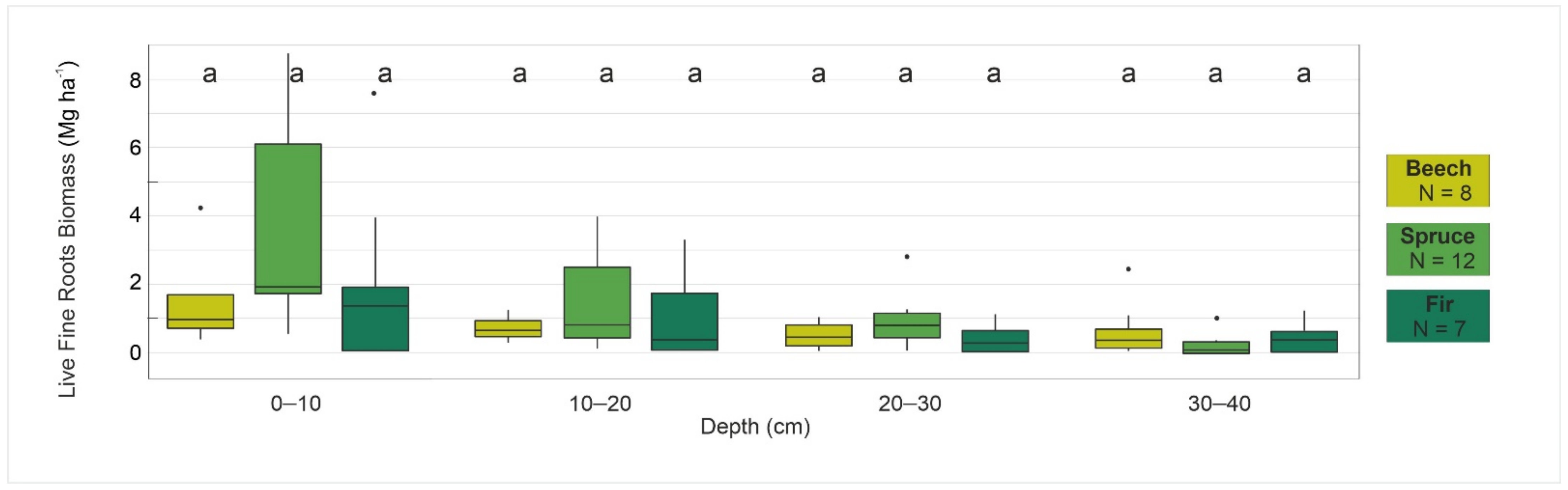
| beech | FRB | 3.2 | 5.5 | 1.2 | 1.2 | 4.1 |
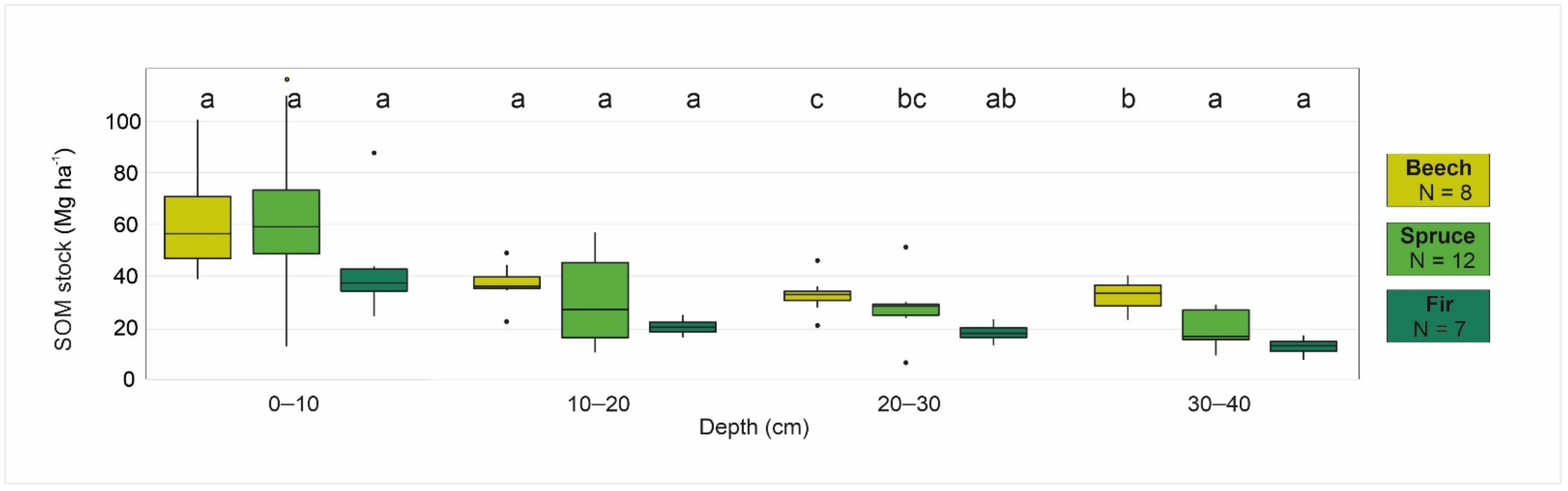
| SOM | 162.9 | 213.3 | 128.5 | 147.6 | 170.1 | |
| spruce | FRB | 3.4 | 10.2 | 0.0 | 1.5 | 3.9 |
| SOM | 142.3 | 224.5 | 56.6 | 124.2 | 162.6 | |
| fir | FRB | 6.5 | 13.8 | 1.2 | 2.3 | 11.0 |
| SOM | 95.5 | 143.3 | 78.6 | 79.3 | 97.6 | |
| Plot Type | Mean | Max | Min | Q1 | Q3 | |
|---|---|---|---|---|---|---|
| beech | C (%) | 47.0 | 56.8 | 37.4 | 40.5 | 51.9 |
| C/N | 46 | 63 | 29 | 39 | 55 | |
| spruce | C (%) | 34.2 | 47.8 | 28.1 | 30.9 | 34.2 |
| C/N | 40 | 52 | 28 | 31 | 47 | |
| fir | C (%) | 40.7 | 50.3 | 26.5 | 32.2 | 49.5 |
| C/N | 40 | 51 | 23 | 32 | 50 | |
| Plot Type | RMSE | r2 | CV | |
|---|---|---|---|---|
| SOM | All plots | 37.57 | 0.22 | 0.31 |
| Beech | 29.51 | 0.74 | 0.18 | |
| Spruce | 23.49 | 0.75 | 0.32 | |
| Fir | 23.49 | 0.75 | 0.24 | |
| FRB | All plots | 2.92 | 0.29 | 0.87 |
| Beech | 1.41 | 0.68 | 0.42 | |
| Spruce | 3.60 | 0.41 | 0.88 | |
| Fir | 4.39 | 0.83 | 0.81 |
Publisher’s Note: MDPI stays neutral with regard to jurisdictional claims in published maps and institutional affiliations. |
© 2021 by the authors. Licensee MDPI, Basel, Switzerland. This article is an open access article distributed under the terms and conditions of the Creative Commons Attribution (CC BY) license (https://creativecommons.org/licenses/by/4.0/).
Share and Cite
Zielonka, A.; Drewnik, M.; Musielok, Ł.; Dyderski, M.K.; Struzik, D.; Smułek, G.; Ostapowicz, K. Biotic and Abiotic Determinants of Soil Organic Matter Stock and Fine Root Biomass in Mountain Area Temperate Forests—Examples from Cambisols under European Beech, Norway Spruce, and Silver Fir (Carpathians, Central Europe). Forests 2021, 12, 823. https://doi.org/10.3390/f12070823
Zielonka A, Drewnik M, Musielok Ł, Dyderski MK, Struzik D, Smułek G, Ostapowicz K. Biotic and Abiotic Determinants of Soil Organic Matter Stock and Fine Root Biomass in Mountain Area Temperate Forests—Examples from Cambisols under European Beech, Norway Spruce, and Silver Fir (Carpathians, Central Europe). Forests. 2021; 12(7):823. https://doi.org/10.3390/f12070823
Chicago/Turabian StyleZielonka, Anna, Marek Drewnik, Łukasz Musielok, Marcin K. Dyderski, Dariusz Struzik, Grzegorz Smułek, and Katarzyna Ostapowicz. 2021. "Biotic and Abiotic Determinants of Soil Organic Matter Stock and Fine Root Biomass in Mountain Area Temperate Forests—Examples from Cambisols under European Beech, Norway Spruce, and Silver Fir (Carpathians, Central Europe)" Forests 12, no. 7: 823. https://doi.org/10.3390/f12070823
APA StyleZielonka, A., Drewnik, M., Musielok, Ł., Dyderski, M. K., Struzik, D., Smułek, G., & Ostapowicz, K. (2021). Biotic and Abiotic Determinants of Soil Organic Matter Stock and Fine Root Biomass in Mountain Area Temperate Forests—Examples from Cambisols under European Beech, Norway Spruce, and Silver Fir (Carpathians, Central Europe). Forests, 12(7), 823. https://doi.org/10.3390/f12070823