Mid-Scale Drivers of Variability in Dry Mixed-Conifer Forests of the Mogollon Rim, Arizona

Jaquette, Matthew; Sánchez Meador, Andrew J.; Huffman, David W.; Bowker, Matthew A.

doi:10.3390/f12050622

Open AccessArticle

Mid-Scale Drivers of Variability in Dry Mixed-Conifer Forests of the Mogollon Rim, Arizona

¹

School of Forestry and Ecological Restoration Institute, Northern Arizona University, Flagstaff, AZ 86011, USA

²

Ecological Restoration Institute, Northern Arizona University, Flagstaff, AZ 86011, USA

³

School of Forestry, Northern Arizona University, Flagstaff, AZ 86011, USA

^*

Author to whom correspondence should be addressed.

Forests 2021, 12(5), 622; https://doi.org/10.3390/f12050622

Submission received: 6 April 2021 / Revised: 28 April 2021 / Accepted: 12 May 2021 / Published: 14 May 2021

(This article belongs to the Section Forest Ecology and Management)

Download

Browse Figures

Review Reports Versions Notes

Abstract

:

The structure and composition of southwestern dry mixed-conifer forests have changed significantly, decreasing forest resiliency to uncharacteristic disturbances which also threaten ecosystem services. Restoration of these forests can be informed by historical conditions; however, managers and researchers still lack a full understanding of how environmental factors influence forest conditions. We investigated historical and contemporary variability in dry mixed-conifer forests in northern Arizona and identified important environmental drivers. We utilized forest sample plots and dendrochronological reconstruction modelling to describe forest conditions in 1879 and 2014, respectively. We used correlogram analysis to compare spatial autocorrelation of average diameter, basal area and tree density, and structural equation modeling to partition the causal pathways between forest structure, forest composition, and a suite of environmental factors reflecting climate, topography, and soil. Historical (1879) reconstructed forests had significantly fewer trees, lower basal area, and higher average diameter than contemporarily (2014). Composition has shifted from ponderosa pine dominance towards a more mixed-species composition. Historically, forest structure did not exhibit strong spatial autocorrelation, but contemporary tree density and diameter were strongly autocorrelated. Environmental factors described little variation in historical forest conditions but are more important for contemporary conditions. Managers can utilize this increased understanding of variation to tailor silvicultural prescriptions to environmental templates.

Keywords:

forest restoration; historical structural conditions; structural equation modelling; correlogram analysis; fire exclusion

1. Introduction

Mixed-conifer forests cover approximately 1 M hectares in the southwestern United States [1] and provide critical ecosystem services such as wildlife habitat [2], watershed protection [3], carbon sequestration, and nutrient cycling [4,5]. However, 20th-century land-use practices, specifically unregulated logging, grazing, and active fire suppression, have disrupted natural fire regimes [6,7,8]. This has decreased these forests’ resilience [9,10]—the “ability of an ecosystem to regain structural and functional attributes that have suffered harm from stress or disturbance” [11]. Disrupting the historical disturbance regimes of frequent, low-severity fires has altered the structure and composition of these forests [12,13,14] and has decreased their resilience to disturbances such as severe wildfire, insects, disease, and climate change [9,10]. Restoring forest structure and composition can increase ecological resilience, and many restoration prescriptions are guided by historical reference conditions [11].

Reliance on historical reference conditions assumes that these characteristics can provide context for managing contemporary ecosystems, and species conservation can be accomplished by approximating the range of environmental conditions present prior to ecological degradation [15]. While there has been criticism that historical conditions will become irrelevant under future climatic conditions [16], restoring a more characteristic composition and structure would increase ecosystem resiliency [3,9] and allow these ecosystems to resist type conversion due to wildfire and climate warming [9,10,17].

In mixed-conifer forests of the American southwest, species composition varies along a temperature–moisture gradient. At one end of the spectrum, ‘warm-dry’ mixed-conifer is dominated by ponderosa pine (Pinus ponderosa) and can include other fire-tolerant/shade-intolerant species such as Gambel oak (Quercus gambelii), Douglas-fir (Pseudotsuga menziesii) and southwestern white pine (Pinus strobiformis). ‘Cool-moist’ mixed-conifer generally lacks ponderosa pine and has a greater composition of fire-intolerant/shade-tolerant species such as quaking aspen (Populus tremuloides), Engelmann spruce (Picea engelmannii), and white fir (Abies concolor) [18]. In the warm-dry type, species composition has shifted towards more shade-tolerant species over the last 100+ years since fire exclusion; ponderosa pine has decreased in dominance and the proportion of southwestern white pine and white fir have increased [12,13,14,19].

Forest density in warm-dry forests has also changed from pre-fire exclusion conditions. Historically, these forests had densities ranging from 51.6 to 245.6 trees ha⁻¹ and basal areas of 7.9 to 28.5 m² ha⁻¹ [9]; however, contemporary forest conditions across the southwest are much denser [12,14,19,20,21,22,23]. These overly dense forests are at an increased risk of burning at high severity in an increasing number of large, uncharacteristic fires across the southwest [24,25]. This contemporary fire regime differs from the natural historical fire regime of frequent, low- to mixed-severity fires [9]. Mean fire return intervals ranged from 2 to 8.5 years on the Mogollon Rim in northern Arizona [13] and to 31.6 years in New Mexico [26] and 32 years in southwestern Colorado [12].

While previous studies have described the natural range of variability, managers still lack full understanding of the relationships that drove historical forest structure. Topography, climate, and soil factors are known to influence forest condition. Topographic models and measures of solar radiation have been used to understand variation in forest structure and composition [27,28]. Climate has strong interactions with fire frequency [12,26,29], and precipitation and climatic water availability drive variation in tree establishment [30,31,32] and density [23,33]. Soil properties, especially parent material, also influence forest structure and composition [23,34,35,36].

Additionally, a more complete understanding of spatial heterogeneity in dry mixed-conifer forests is needed. Variability in forests is spatially structured and hierarchically organized [9,23,37]. Fine-scale (<4 ha) spatial patterns typically describe the arrangement of individual trees within a stand and are nested within mid-scale (4–400 ha) patterns, which describe the variation among stands within a landscape. Mid-scale patterns are further nested within landscape-scale (400+ ha) structure. A review of spatial analyses in fire-frequent forests found that most spatial analyses of reference conditions have focused on fine-scale tree patterns of clusters of trees, single trees, and openings that manifest at scales from 0.4 to 4 ha [9]. However, such patterns might be difficult for forest managers to implement in stand-level treatments [37]. Landscape restoration projects that solely focus on fine-scale patterns risk creating landscapes that are heterogeneous at fine scales, but homogeneous over mid- to landscape scales [38]. The lack of mid-scale heterogeneity analyses in southwestern dry mixed-conifer forest limits managers from designing appropriate restoration projects.

Our study addressed these knowledge gaps by investigating drivers of historical variability in dry mixed-conifer forests on the Mogollon Rim in northern Arizona. Specifically, we focused on answering the following research questions: (1) What were the historical structural conditions in these ecosystems? (2) How did structural conditions vary spatially, and has spatial variation changed since fire exclusion? and (3) What were the drivers of variability in these forests, and how have drivers changed in relative importance since fire exclusion? Answers to these questions can help silviculturists design restoration treatments that have appropriate levels of spatial and structural variability and better reflect environmental templates. By analyzing forest variability of historical and contemporary time periods, we can further explore how fire exclusion has impacted these forests.

2. Materials and Methods

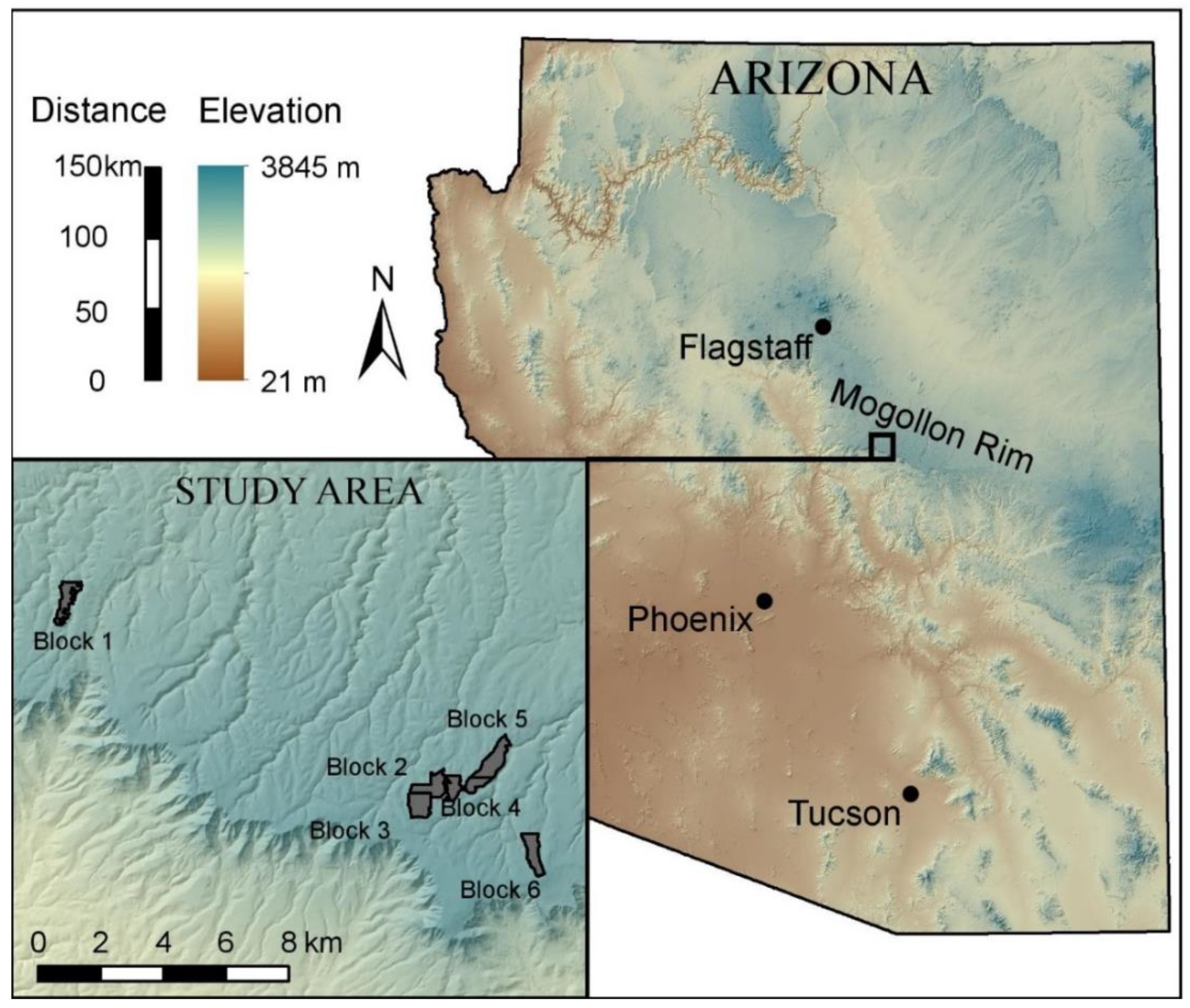
2.1. Study Design

The Mogollon Rim is an escarpment stretching approximately 320 km from northern Arizona to eastern Arizona and forms the boundary between the Colorado Plateau to the north and the Southern Basin and Range Province to the south [39]. Our study area on the Mogollon Rim ranges from 2223 to 2399 m in elevation, has a mean annual temperature of 9.3 °C and a mean annual precipitation of 89 cm (Table A1). The forests fall into the warm/dry classification of mixed-conifer forest [18], with a major component of ponderosa pine, and a mixture of southwestern white pine, Douglas-fir, white fir, Gambel oak, and quaking aspen. Additional tree species found on the Mogollon Rim include New Mexico locust (Robinia neomexicana) and bigtooth maple (Acer grandidentatum) [19]. Low-severity fires burned frequently on the Mogollon Rim with a mean fire interval of 2 to 8.5 years until 1879 [13]. The forests on the Mogollon Rim are currently the target of restoration efforts to increase ecological resilience [40] and protect important municipal water supplies [41].

This study utilized existing pre-treatment data collected from the long-term ecological assessment and restoration network (LEARN) which was established in 2014 by the Ecological Restoration Institute, in coordination with the U.S. Forest Service Mogollon Rim Ranger District of the Coconino National Forest (see Figure 1). The surveyed area covers approximately 250 ha, broken into six blocks where each block consisted of three ~16 ha treatment units with 15 0.04-ha circular, fixed-radius plots arranged on a 60-m grid within each unit for a total of 270 plots across the study area. Crews completed data collection in 2014, following methods described in detail in Roccaforte et al. [42]. Surveys recorded species, diameter at breast height (DBH: 1.37 m above the ground), diameter at stump height (DSH: 40 cm above the ground), total height, height to the base of the live crown, two crown radii measurements (long and short side) and condition (live tree, snag, log, cut stump, etc.) of all trees taller than breast height and all dead trees that may have predated Euro–American settlement (ca. 1879). Crews collected tree cores on all pre-settlement trees, trees larger than 40 cm DBH, and 10% of all trees smaller than 40 cm DBH.

2.2. Determining Historical Variability

To determine the historical variability at our site in the dry mixed-conifer forests of the Mogollon Rim, we reconstructed historical forest structure and composition using field plot data and dendroecological reconstruction techniques. These techniques were developed and discussed in detail most recently by Rodman et al. [19] to incorporate additional species. This reconstruction model estimated the diameter of each tree during a set reconstruction year. We used 1879 for the reconstruction year, as a nearby by study [13] reported this to be the date of fire regime disruption. Historical tree diameters were based on dendrochronological data (i.e., cross-dated increment cores collected from trees on field plots—see above) when available, and species-specific “back-growth” regression equations when dendrochronological data was not available. These “back-growth” equations estimated the historical diameter using species-specific growth and bark thickness [43] equations. Historical diameters for dead trees were estimated by using current diameter and decomposition equations based on snag/log condition classes to determine death date [44], and then input into the “back-growth” equations to estimate the diameter during the reconstruction year. Cut stumps were assigned death dates of either 1965 or 1981, corresponding with observed releases in tree growth [45] and harvesting operations on the Mogollon Rim [19]. While this method of reconstructing forest structure may fail to detect some small trees that died and decomposed prior to the contemporary surveys, comparisons to historical surveys indicate that 91 to 94% of pre-settlement trees can be identified by contemporary surveys in areas lacking recent disturbance [46,47].

We used the results of the reconstruction model to summarize average diameter (DBH; cm), tree density (trees ha⁻¹), and basal area (m² ha⁻¹) for each field plot. We quantified composition by calculating the ecological importance value (EIV; Equation (1)) of each species in each plot, as described by Curtis and McIntosh [48]. EIV describes the importance of a given species by accounting for its relative density (abundance) as well as relative basal area (dominance), of the species. This index ranges from 0 to 2 and is calculated using the following equation:

{EIV}_{spp} = \frac{n_{spp}}{n_{total}} + \frac{{BA}_{spp}}{{BA}_{total}}

(1)

where EIV_spp is the species-specific ecological importance value; n_spp and BA_spp are the species-specific tree density and basal area, respectively; and n_total and BA_total are the total tree density and basal area, respectively. We summarized these measures of forest structure and composition across all study plots to determine the historical variability, as well as the contemporary conditions at our Mogollon Rim site.

2.3. Measuring Spatial Variability

We evaluated spatial variability across the study area by quantifying spatial autocorrelation. We used the ‘spdep’ package in R [49,50] to calculate Moran’s I [51,52]. We chose to use Moran’s I to evaluate spatial variability because this metric is useful for describing patterns of continuous phenomena, estimating the size of patches, and is commonly used in research (e.g., [14]). Significant values of Moran’s I indicate positive and negative correlations between the attributes of interest for geographically compared plots [53]. We calculated Moran’s I for average diameter, tree density, and basal area and then compared the empirical values at specified distances (lags) to simulations of expected values given no significant autocorrelation to evaluate significance.

When calculated globally (i.e., across the entire study area) Moran’s I describes the spatial autocorrelation of a variable—that is, whether the variable is distributed independently across a landscape or is dependent upon the value of its neighbors. When calculated locally, Moran’s I can also be plotted over increasing lag distances to create a correlogram, describing the lag distance at which observations are highly correlated or exhibit spatial autocorrelation. We calculated a local Moran’s I over 17 lags, where each lag generally represents the 60 m distance between survey plots. Comparing the correlograms of the historical and contemporary data, we visually evaluated whether spatial variability had changed since the exclusion of natural frequent fire regimes.

The arrangement of the experimental blocks at the study site posed a challenge to using Moran’s I in our analysis. Ideally, we could evaluate a complete range of distances up to the maximum distance between any two points in the study area. However, there are significant gaps between some blocks. Blocks 2 through 5 are contiguous but Blocks 1 and 6 are disjunct from the others (see Figure 1). In Blocks 1 and 6, Moran’s I cannot be calculated across distances larger than the maximum distance within the block, so we limited our analysis to 1000 m, approximately the distance across one block. While this hinders our ability to make inferences about landscape spatial patterns, we were still able to evaluate variability across mid-scales.

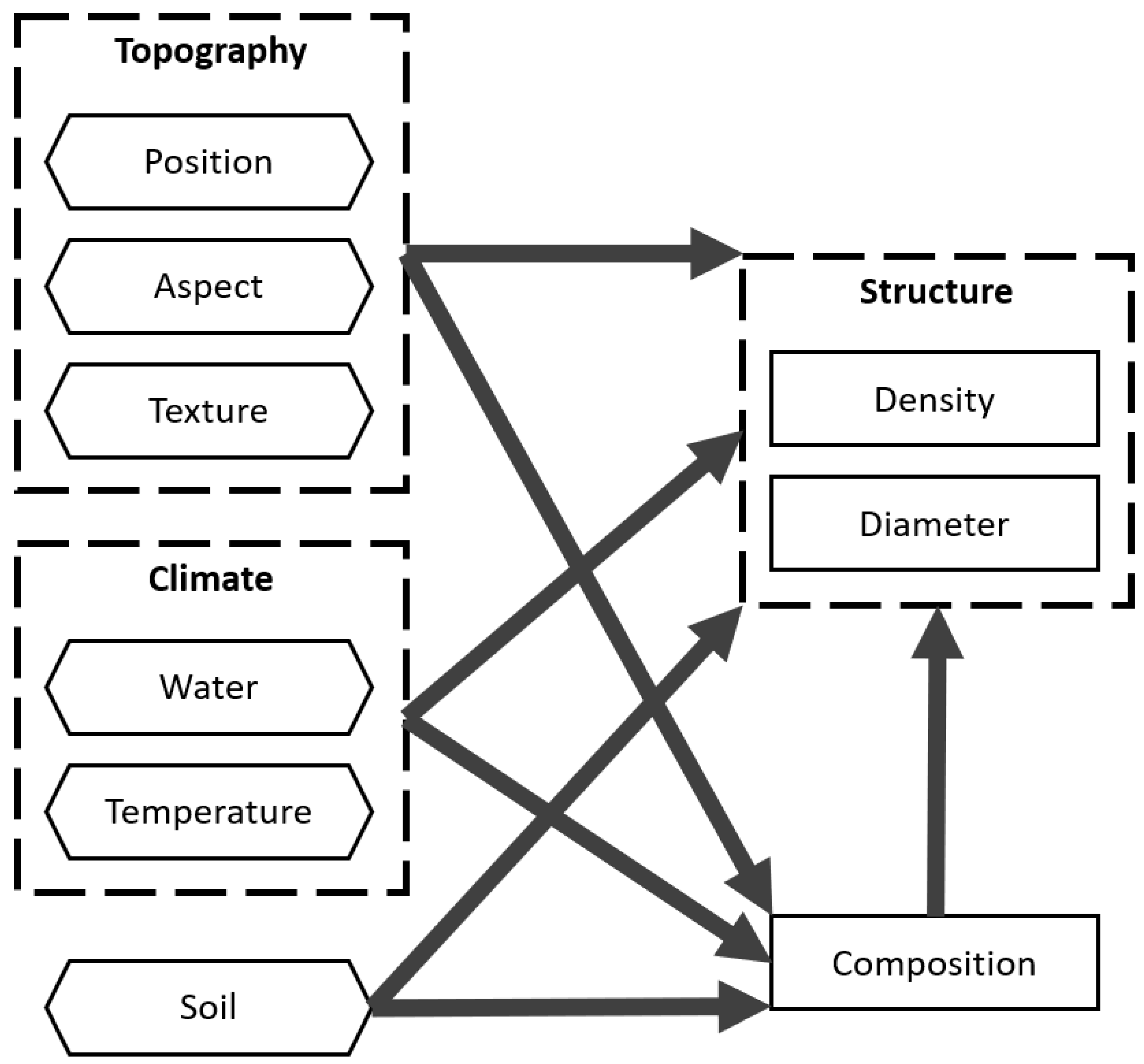
2.4. Identifying Drivers of Variability

We used structural equation modeling (SEM) techniques in Amos software [54] to identify the important relationships between environmental factors and forest structure and composition that drove variation at the study site. SEM is an analytical framework useful for investigating complex ecological systems because it can model multivariate relationships, explicitly partition direct and indirect causal relationships, include unmeasured concepts as latent or composite variables, and provide a test of causal inferences [55,56]. SEM has been successfully used in southwestern forests to understand ponderosa pine regeneration [32] relationships between environmental conditions, fire history, and understory species richness and abundance [57,58] and to explore the drivers of plat-animal interactions [59]. We chose to use SEM in our analysis to evaluate the relative importance of abstract environmental factors, and to explicitly incorporate the relationship between structure and composition as an indirect causal relationship.

To evaluate the relationships between environmental factors, forest composition, and forest structure, prior to and following fire regime disruption, we built two independent models using reconstructed and contemporary field plot conditions. These two models followed the same model building techniques, and started from the same a priori model, but used separate historical and contemporary datasets. While we could have tried multi-group modeling, which would focus on determining which pathways differ most between time periods [60], we were more interested in precise estimates of the effects of the drivers of variability, optimized for each time period.

Our conceptual model describes our hypothesis that environmental factors directly influence forest structure and composition, and indirectly influence forest structure through composition (see Figure 2). Measured variables were grouped into three broad environmental factors: topography, climate, and soils. The measured variables of each environmental factor were all correlated to each other (not shown in Figure 2 for simplicity). Each factor could have been represented by many measures, so we compiled a large pool of potential explanatory variables to select from (see Table A1 for a complete, detailed list of explanatory variables).

We used composite variables extensively as predictors of forest properties. Composites are an interpretational tool that can be used to compile the influences of multiple conceptually-linked variables into one composite effect. Topographic variables were based on a high-resolution (1 m × 1 m), LiDAR-derived digital elevation model (DEM), and were calculated at 10 m resolution in ArcMap 10 software [61] and in R (version 3.6.1) statistical software using the ‘raster’ [62] and ‘SpatialEco’ [63] packages. In the conceptual model we selected from Beer’s aspect (or northeastness) [64], the heat load index (HLI) [65], and the solar radiation index (SRI; calculated for the years 1879 and 2014) [66] to represent ‘aspect’ as a composite variable; we selected from elevation, topographic slope position (TPI), and hierarchical slope position (HSP) to represent ‘position’ as a composite variable; and we selected from slope, roughness, and the topographic ruggedness index (TRI) [67] to represent ‘texture’ as a composite variable (Figure 2).

Climate factors included seven different climate variables: precipitation, mean temperature, minimum and maximum temperatures, mean dewpoint temperature, and maximum and minimum vapor pressure deficits. These data were acquired from the Parameter-elevation Regressions on Independent Slopes Model (PRISM) [68] for each month in 30 year periods from 1895 to 1924 (historical climate) and 1981 to 2010 (contemporary climate). PRISM data were used in ecological analyses where weather data have not been collected on site. We spatially downscaled climate variables from their native 800 m × 800 m resolution to the plot level resolution (60 m × 60 m) using gradient and inverse distance-squared weighting methods as described by Rodman et al. [23]. The downscaled climate variables were summarized as annual averages and seasonal (e.g., summer = 1 June–31 August) averages for the 30-year periods and assigned to each corresponding plot. In the conceptual model we selected from precipitation, dewpoint temperature, minimum and maximum vapor pressure deficit variables into a ‘water availability’ composite variable; and selected from mean, minimum and maximum temperature variables into a ‘temperature’ composite variable (Figure 2).

Soil parent material is known to influence forest conditions [23,35]; however, parent material does not vary substantially across the study area. Data from the Natural Resources Conservation Service’s Soil Survey Geographic database (SSURGO) indicated that the entire study area was Kaibab Limestone residuum [69]. In lieu of parent material, we used soil characteristics that do vary across the study area and are still important drivers of forest conditions [32,59]. Soil variables were calculated from the SoilGrids 100 m dataset [70]. Soil variables included six soil properties—percent organic C, total N, bulk density, pH, percent sand, and percent clay—at seven standard soil depths—0, 5, 15, 30, 60, 100, and 200 cm. We selected from all these variables to represent a ‘soil’ composite variable (Figure 2).

We used average diameter and tree density from the historical reconstruction and the contemporary survey as indicators of forest structure in the SEMs. To represent forest composition in the SEMs, we used distance-based ordination techniques to reduce the complexity of the community data so that they would be easier to use in variable selection and structural equation modeling. We used the ‘vegan’ package [71] in R for this analysis. We transformed and standardized plot-level species count data before calculating Bray–Curtis distance to describe the differences between plot overstory communities. We then used nonmetric multi-dimensional scaling (NMDS) to calculate an independent three-axis solution for both the historical and contemporary community data and to calculate species scores within ordination space. Each three-axis solution was rotated to place the maximum variation along the first axis, which we then used to summarize the community composition of each plot (see Appendix B for a more complete description of this approach). Transformed average diameter, transformed density and the first axis scores from the community NMDS, make up the response variables for both our historical and contemporary models.

With more than 100 potential explanatory variables to include in each model, but desiring to keep the models parsimonious, we selected explanatory variables from each category to build each composite variable based on correlation with the response variables. We selected variables with the strongest correlations (i.e., greater than 0.1 or less than −0.1), making sure not to select redundant variables (e.g., the same soil characteristic at multiple depths, or the same climate variable at multiple seasons).

Using these criteria, we identified eleven measures of topography, climate, and soil to include in both the historical and contemporary models. For the topography factor, we selected hierarchical slope position to represent position, the solar radiation index to represent aspect, and the topographic ruggedness index to represent texture. We selected percent organic C at 30 cm, pH at 0 cm, and percent clay at 30 cm to represent the composite soil factor. For the composite climate factor, we selected winter minimum vapor pressure deficit and spring precipitation to represent water, and fall mean temperature, and winter maximum and minimum temperatures to represent temperature. For the contemporary model, we identified nine measures of topography, climate, and soil to include in the model. For topography, the same factors (HSP, SRI, and TRI) were selected. We selected pH at 0 cm, and percent clay at 30 cm to represent the soil factor. For climate, we selected spring precipitation and summer mean dewpoint temperature to represent water, and winter minimum and maximum temperatures to represent temperature.

After variables were selected, we verified the linearity of relationships before making necessary modifications to the model. To simplify the model where possible, we replaced all of the topography composite variables (aspect, position, and texture), which had only one explanatory variable, with direct effects. We found multicollinearity between the explanatory variables of ‘temperature’ and ‘water’ which may have caused path coefficient inflation in the model. This issue was resolved by combining these two factors into a single ‘climate’ composite. While our approach of correlating all environmental variables was conservative, this saturated the model, and model fit statistics could not be calculated with any spare degrees of freedom. To evaluate model fit we removed the least significant correlation from the model, and calculated three model fit statistics (chi-squared goodness-of-fit, Chi²; an adjusted goodness-of-fit index (AGFI); and root mean square error of approximation, RMSEA) over one degree of freedom. Because there were no significant correlations in the paths removed, the final models behaved essentially the same as a saturated model. While saturated models are traditionally not used as the final SEM, this was appropriate in our analysis because our objective was to evaluate the relative importance of the environmental factors rather than test a novel theory of hypothesized relationships in the ecosystem.

3. Results

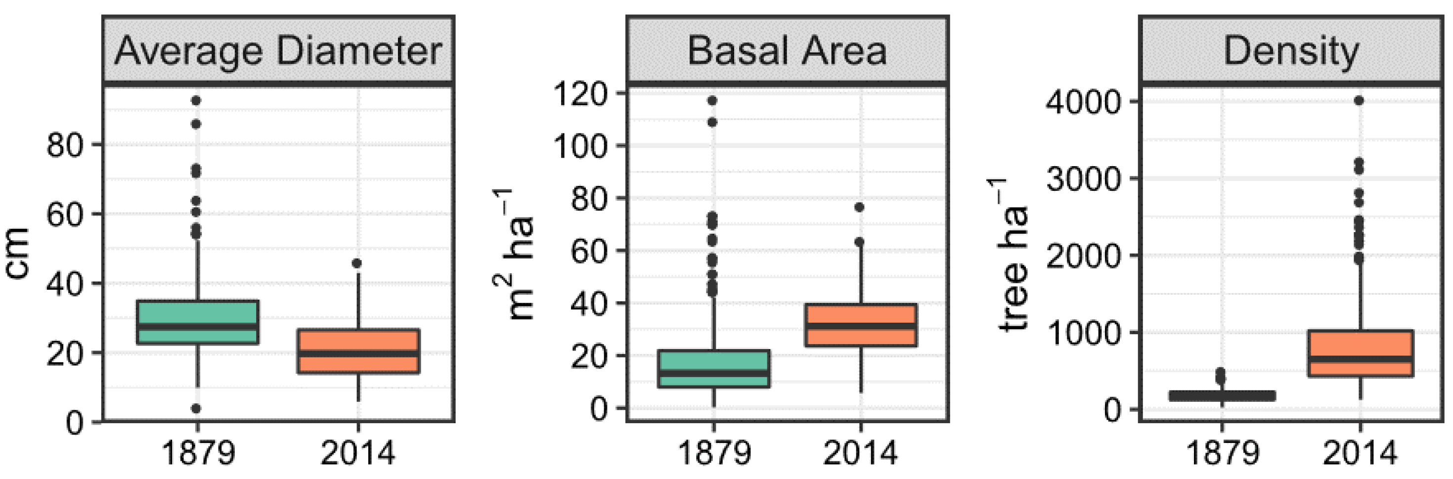
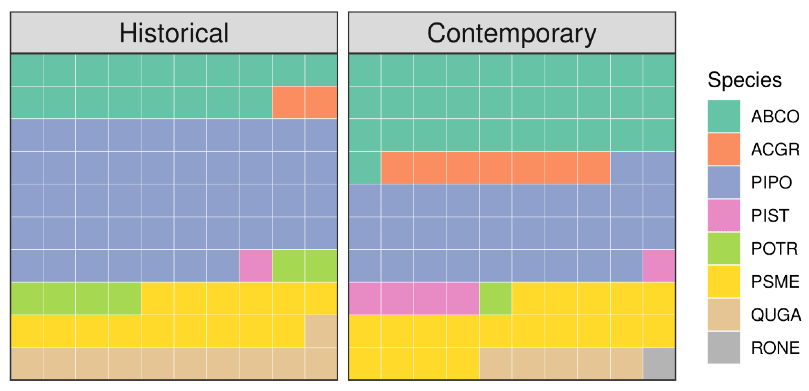
3.1. Historical and Contemporary Conditions

Historical forest conditions prior to fire regime disruption (1879) differed significantly from contemporary conditions in 2014 (Figure 3). Mean tree diameter across the study sites averaged 27.5 (95% CI: 13.3–57.0) cm historically and varied widely across sample plots. Contemporary average tree diameter was significantly lower (p < 0.0001) than historical conditions and averaged 20.1 (7.4–39.0) cm.

In 1879, basal area averaged 12.6 (2.0–79.4) m² ha⁻¹ (see Figure 3 and Figure 4). Historical basal area was highly variable but significantly lower than contemporary basal area (p < 0.0001). Contemporary basal area averaged 30.8 (12.0–58.3) m² ha⁻¹ (see Figure 3 and Figure 4). Historical forests had an average density of 165 (48–352) trees ha⁻¹. Comparisons with contemporary forest were found to be significantly denser (p < 0.0001), with an average density of 657 (188–2302) trees ha⁻¹.

Historically, forest overstory composition was typical of dry mixed-conifer in the southwest (Figure 5). Ponderosa pine accounted for approximately half of total EIV (0.934/2.0; see Equation (1)), with minor components of white fir (EIV: 0.368), Douglas-fir (EIV: 0.302), and Gambel oak (EIV: 0.214). Contemporary composition is also characteristic of dry mixed conifer, though ponderosa pine was found to have decreased in importance (EIV: 0.622) and there has been a shift towards more mesic species. For example, white fir now accounts for approximately one-third of total EIV (0.620/2.0), Douglas-fir increased to 0.370 EIV, and southwestern white pine increased from 0.018 in 1979 to 0.102 EIV in 2014. There were also changes in the relative dominance of sprouting deciduous trees: Gambel oak (0.214 to 0.106) and aspen (0.118 to 0.008) decreased; bigtooth maple and New Mexico locust increased (0.042 to 0.146; and 0.004 to 0.024, respectively).

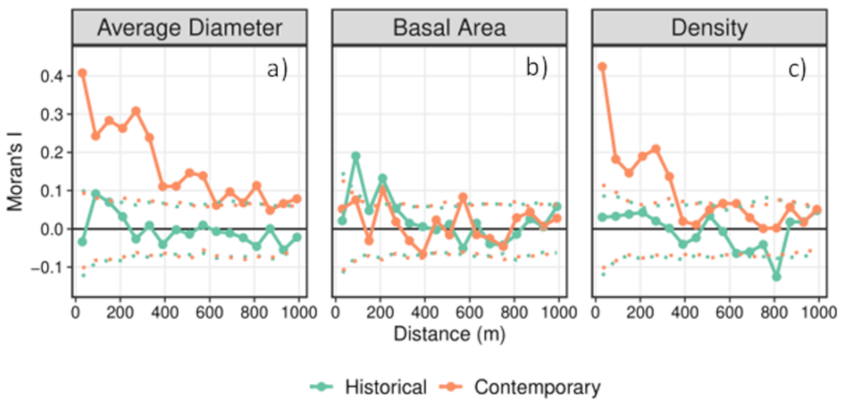
3.2. Spatial Variability

Overall, we found little indication of spatial autocorrelation in historical forest structure, suggesting homogeneity of conditions. This homogeneity can be seen in the maps of historical forest structure (e.g., Figure 4). Historically, average diameter had low Moran’s I and fell within the envelope of no significant spatial autocorrelation at all distances (Figure 6a). Basal area was significantly autocorrelated at distances of 90 and 210 m but at all other distances was within the envelope of no significant spatial autocorrelation (Figure 6b). Interestingly, density was significantly negatively autocorrelated at 810 m, but was otherwise not significantly autocorrelated at all other lags. (Figure 6c).

Unlike historical conditions, some contemporary conditions exhibited significant spatial autocorrelation. Average diameter was highly autocorrelated over distances of 0 to 360 m and significantly autocorrelated at distances up to 1000 m (Figure 6a). Tree density was significantly autocorrelated in contemporary forests at distances up to 360 m and showed slight autocorrelation again at approximately 600 m, but was otherwise insignificant (Figure 6c). Unlike average diameter and density, contemporary basal area remained largely uncorrelated, only showing slight autocorrelation at distances of 210 and 570 m (Figure 6b).

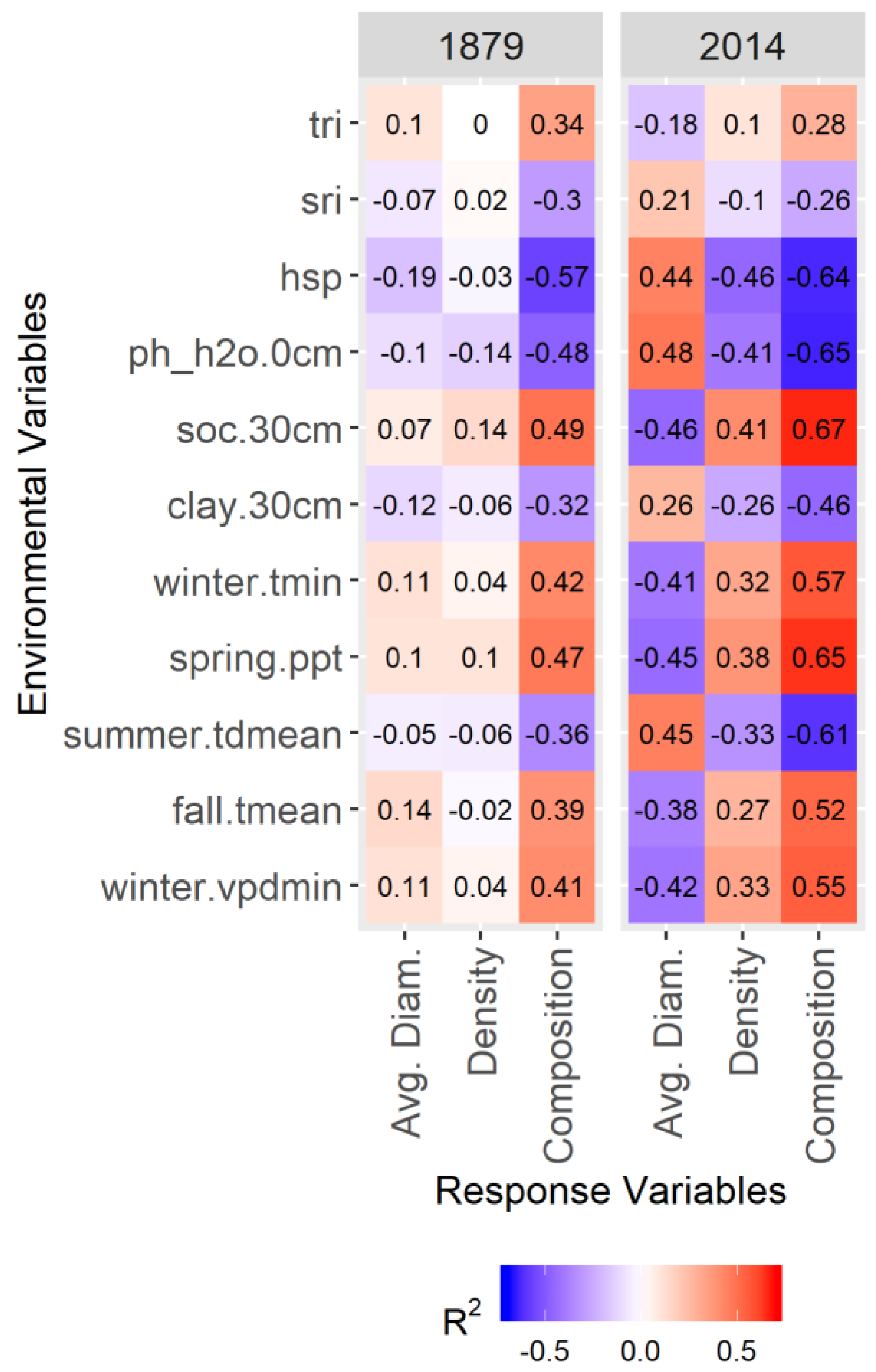
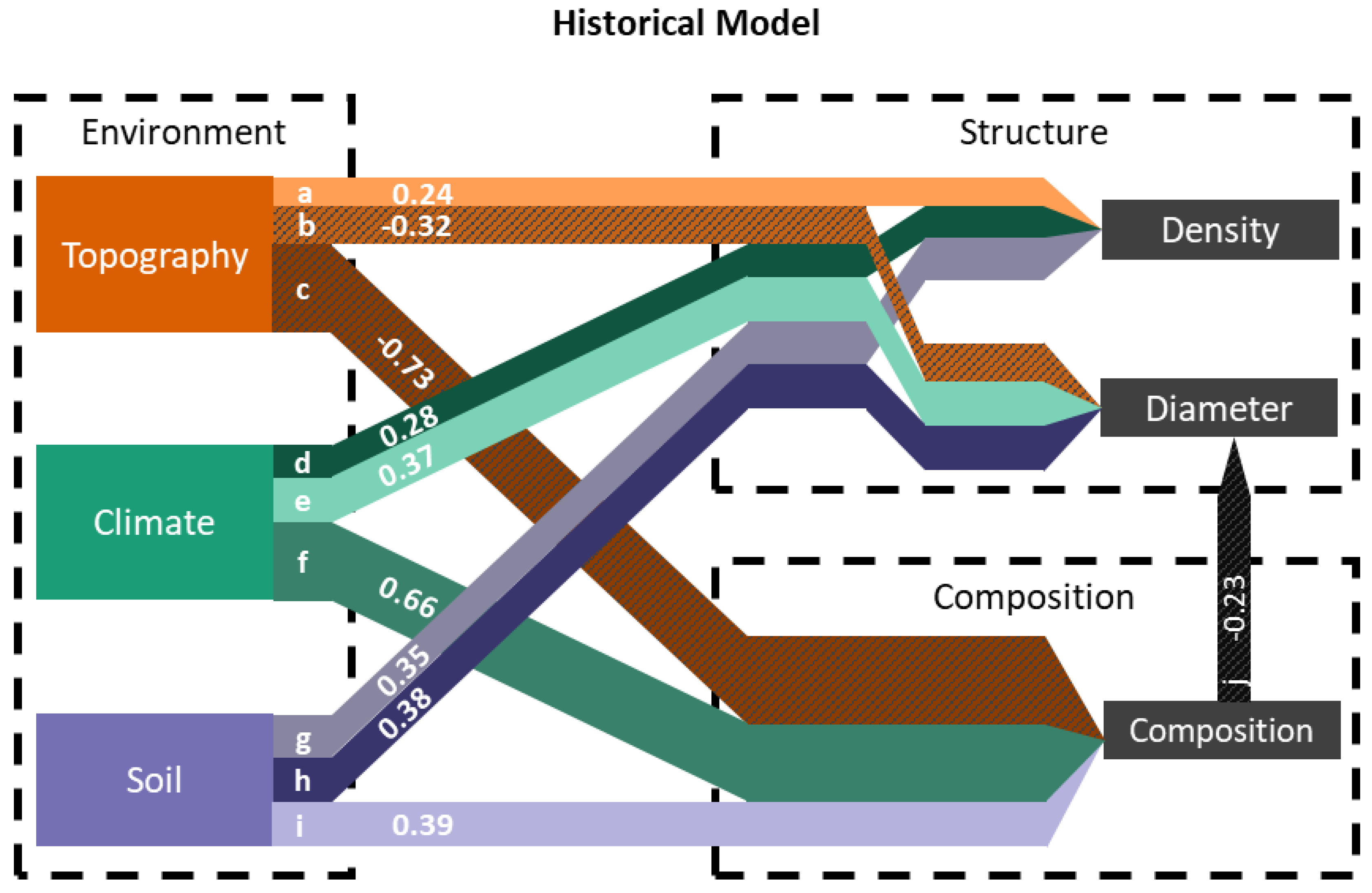
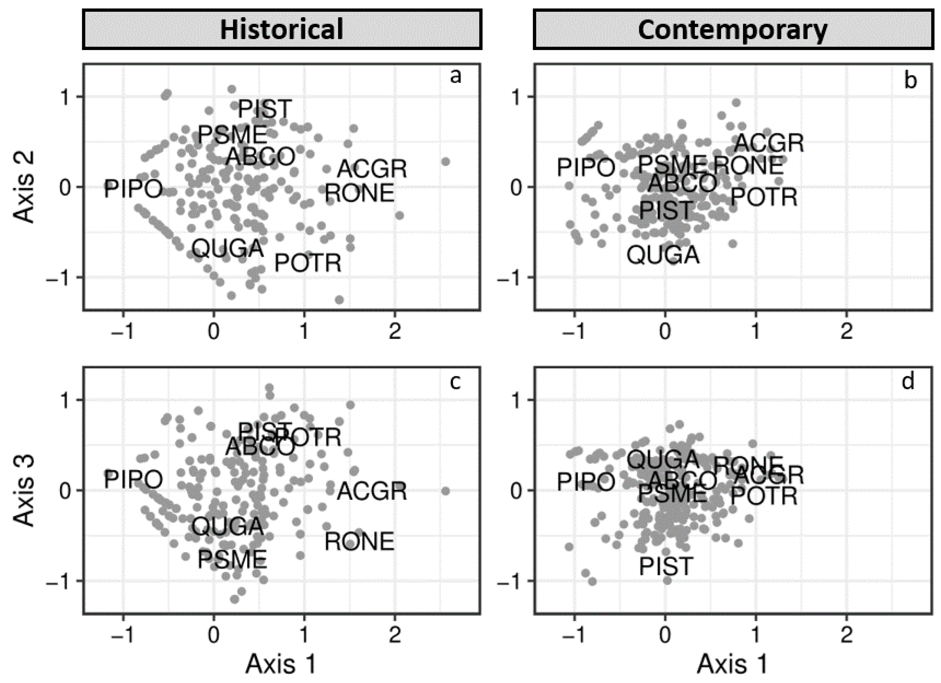
3.3. Drivers of Variability

In both the historical and contemporary datasets, environmental variables exhibited stronger correlations with composition as compared to structure or composition and historical correlation coefficients were generally lower than contemporary values (Figure 7). Additionally, the relationships between average diameter and most environmental variables switched signs, changing from weakly positive to moderately negative, or weakly negative to moderately positive between historical and contemporary time periods (Figure 7).

The Chi², RMSEA, and AGFI evaluations of model fit suggest that the historical SEM adequately fit our data (see Table 1). In these tests the p-value indicates the probability of good fit; commonly, p > 0.05 is considered adequate, though this is only convention. The AGFI has no p-value; commonly, an AGFI > 0.95 is interpreted to represent a good-fitting model, but again, this is only convention. The historical model has good descriptive power for composition (r² = 0.483) but has low descriptive power for average diameter (r² = 0.088) and basal area (r² = 0.101).

Topography and climate factors had relatively high importance in driving historical forest structure and composition, while soil factors had a lower impact on forest conditions (see Figure 8). The climate–composition relationship had the highest single path coefficient in the historical model (total absolute value of the path coefficient: 0.66), while topography has a higher overall impact on historical composition than climate, from the cumulative effect of aspect, position, and texture (0.73). Climate was a significant driver of historical density (0.28) and diameter (0.37) but was of approximately equal importance with topography for these structural variables (0.24 and 0.32, respectively). Aspect and texture were not significant drivers of tree density or diameter. Soil had an impact on historical density (0.35) and diameter (0.38) that was similar to that of climate and topography. Soil had a relatively small, though still significant, impact in driving historical forest composition (0.39). Composition did not significantly drive variation in historical tree density but did have an impact on average tree diameter. While statistically significant, this path coefficient (−0.23) was the smallest driver of historical average diameter. See Appendix A Table A2 for full details of the resulting model path components.

For our contemporary model, Chi², RMSEA, and AGFI results also suggest that the contemporary model converged at a solution with good fit (Table 1). The model had good descriptive power for density (r² = 0.296) and diameter (r² = 0.317), and even better description of forest composition (r² = 0.632). In the contemporary model (Figure 9), climate factors had the strongest relative importance for composition, while topography had the highest relative importance for forest structure. The pathway from climate to composition had the strongest total absolute value of a path coefficient in the model (0.79) while pathways that lead from climate to density (0.21) and average diameter (0.21) had relatively low importance. Topography had the strongest influence on contemporary forest density (−0.36) and average diameter (0.32). Like the historical model, neither aspect nor texture were significant drivers of contemporary forest structure. The cumulative effects of position and aspect on composition (−0.59) was a relatively important pathway. However, texture was not an important driver of contemporary composition. Soil had a relatively weak importance to both contemporary forest density (0.20) and diameter (0.26); this differs from the historical model, where soil was a relatively equal driver of forest structure. The pathway from soil to composition (0.35) was the weakest driver of contemporary composition. The relationship between contemporary forest composition and structure differed from the one suggested by the historical model. Contemporarily, composition was a significant driver of forest density (0.26), but not forest diameter. See Appendix A Table A2 for full details of the resulting model path components.

4. Discussion

4.1. Historical Range of Variability

Our results suggest that the abrupt disruption to the historical frequent fire regime drastically altered the forests on the Mogollon Rim, as has been reported in dry mixed-conifer forests across the southwest (e.g., [12,19,20,21,22,23]). Reconstructed plots showed low density, with large and variable tree sizes and low, yet variable, basal area. The historical variability we found was similar to the ranges reported by both Reynolds et al. [9] and Wassermann et al. [72] for dry mixed-conifer forests in the southwest. Additionally, the average basal area and tree density we found were slightly higher than those reconstructed elsewhere on the Mogollon Rim [14,19] and in the San Juan mountains of southwestern Colorado [12]. Historical dry mixed-conifer forest at the Grand Canyon were reported to be denser than those we found in our study [20,39] and those reported by Williams and Baker [73] for the Mogollon Rim. When compared to mixed-conifer reference conditions outside the southwest, our results are similar to those found on the Front Range of northern Colorado and southern Wyoming [74,75], and considerably less dense than the results reported from some parts of the Sierra Nevada in California [76]. Historical conditions from other parts of the Sierra Nevada [33,77,78] and mountains in Oregon [79,80,81] had higher basal area and lower tree density than in our study area, suggesting that those forests had fewer and larger trees than those found on the Mogollon Rim.

Contemporary forest conditions diverged significantly from historical in all three measures of forest structure. Average diameter was significantly lower in contemporary conditions, reflecting the legacy of harvesting larger trees for timber and the influx of many small trees due to fire exclusion originating in the mid-1900s [14]. Basal area and tree density increased significantly. These changes are consistent with other studies in dry mixed-conifer forests across the southwest; Fulé et al. [20], Heinlein et al. [22], Rodman et al. [19,23], and Strahan et al. [14] all recorded large increases in tree density and basal area in dry mixed-conifer forests over a similar time frame.

We found a shift in forest composition away from dry mixed-conifer, towards a more wet mixed-conifer composition. For example, ponderosa pine has decreased in importance (EIV), while white fir has increased greatly. Southwestern white pine and Douglas-fir have also showed modest increases in EIV. This trend has been previously reported for forests of the Mogollon Rim [13,19] and in other mixed-conifer forests in the Southwest [14,20,22,26]. Our results parallel those of other studies concluding that frequent fires kept mesic, fire-intolerant species in check, but when released from fire they established and survived in areas where they were previously excluded [9,13].

4.2. Changes to Spatial Patterns

Changes to forest structure and composition were accompanied by changes to the spatial pattern to forest conditions, as indicated by our correlogram analysis. Prior to fire regime disruption, the forests on the Mogollon Rim exhibited little significant spatial autocorrelation across scales up to 1000 m (~314 ha). Similarly, Strahan et al. [14] found no significant autocorrelation at similar resolutions, and at distances up to 2500 m in mixed-conifer forests near our site. Both random and aggregated fine-scale patterns have been found on the Mogollon Rim [19,23], as well as outside the southwest [76,82]. Random arrangement of forest structural conditions suggests multi-scalar-level structural heterogeneity that has been theorized [9,37], but not well documented.

In our study, contemporary average diameter and tree density were strongly autocorrelated at distances up to 360 m, suggesting that these forests were composed of large homogeneous patches, approximately 40 ha in size. This distance likely reflects the scale of variation for environmental patterns related to geomorphic features (e.g., ridges and valleys) on the study landscape. Autocorrelation at distances up to 1000 m indicated low variation between patches. Interestingly, basal area showed no autocorrelation despite both average diameter and tree density being autocorrelated. Disruption to the natural frequent fire regime, which maintained historical forest patterns, is the likely explanation for this change. Strahan et al. [14] described a similar shift in the mid-scale variability of community traits, and reported significant spatial autocorrelation up to 250 m. Managers seeking to restore historical spatial patterns should break up large and homogeneous stands into smaller, variable patches, and restoration prescriptions should aim to generate random structural variation within landscape patches. Silvicultural treatments such as group selection or variable density thinning may achieve these goals.

4.3. Drivers of Variability

Our model of historical drivers of variability had poor explanatory power for describing variation in forest structure, and moderate power for composition. This weak relationship between environment and forest structure was also seen in low bivariate correlations between average diameter, density and almost all environmental predictors. Low variation in historical density may have been due to the natural fire regime of frequent, surface fires. Indeed, fire may have been the main driver of historical variability and diminished importance of environmental factors in determining tree size and stand basal area. However, we were unable to include site-specific measures of fire in our model, and the relative importance of fire versus environmental factors in determining historical structure and composition needs further research.

In our model, climate and topography were the main drivers of historical variation in forest structure and composition. Path coefficients indicated that warm and dry winters, high spring precipitation, and warm fall temperatures correlated with low ponderosa pine dominance. Microsites with higher water availability had higher tree densities, and sites with cold, dry winters were associated with larger trees. Winter temperatures influence snowpack duration into the spring and may in turn determine forest density [33]. Spring precipitation is important for ponderosa pine seedling establishment in some forests [31], while fall temperatures may influence fuel moisture and wildfire behavior. Over longer periods, climate can affect fuel availability and timing of widespread fire years in mixed-conifer forests [12,26,29].

Topography was an important driver in our model of historical variation. Slope position was consistently important, reflecting the effects of microsite variability on forest conditions [27,83]. Aspect also drove variation. Sites with more solar radiation dry faster, and drought-tolerant species such as ponderosa pine and Gambel oak are better able to occupy these sites. Drying could also affect the availability of fuels for combustion and in turn affect fire frequency. Interestingly, Rodman et al. [23] did not find topographic factors to be important in determining historical forest structure at sites near ours, nor did Abella and Covington [34] at other sites in northern Arizona. The systematic sample grid in our study area may have captured a wider range of topographic conditions and greater variation in structure and composition than these previous studies.

To evaluate how the relative importance of drivers of variability may have changed, we compared historical and contemporary models. A major difference between the two models was that they describe forests with and without fire. In addition, other disturbances were present during the contemporary period including livestock grazing and selective logging. We were not able to include these processes in our contemporary model. In addition, we did not have measures of natural disturbances such as insect or disease outbreaks, droughts, or wildfires in either model. Such mortality factors would contribute to variation in forest density and composition. Without plot-level measures of these disturbances, we assumed they affected all plots equally, and were confounded with other changes that occurred between 1879 and 2014, such as fire regime disruption and climate change.

Soil was a relatively unimportant driver of variability in both historical and contemporary models. However, Rodman et al. [23], Abella and Denton [35], Kimsey et al. [36], and Laughlin et al. [58] demonstrated that soil parent material drove significant variation in forest structure and composition at northern Arizona sites. The limited variation in soil parent material across our study site likely explains our findings.

Interestingly, environmental factors exhibited a stronger influence on contemporary forest conditions than on historical structure and composition, possibly due to anthropogenic exclusion of frequent fire. The contemporary model had stronger explanatory power than the historical model, which reflected stronger correlations between contemporary environmental variables and forest measures. Climate was distinctly the most important driver of forest composition on the contemporary landscape, and indicated that sites with high spring precipitation, cold winter low temperatures, and dry summers were associated with low ponderosa pine dominance. Forest composition may have historically been constrained by species adaptedness to fire, but in the absence of fire climate asserted greater control of forest composition. Similar responses to fire exclusion have been described in other studies [9,13,14,19,20]. We found that climate increased in relative importance contemporarily, and different components of climate became important. Similarly, Mueller et al. [84] described a strengthening fire-climate relationship, and others have reported changes in the timing of widespread fire years relative to periods of drought or above average precipitation since fire regime disruption [85,86].

Topography was less important to contemporary forest composition than in the historical period, perhaps because microsite–fuel relationships [83] were less important. Topography was the strongest driver of both tree density and diameter, but this relationship changed dramatically since fire exclusion. While lower slopes and valleys historically had lower density and larger trees, contemporarily they were dominated by high densities of smaller trees. Historical logging targeted large, commercially valuable trees, which may have been concentrated on lower, more productive microsites. While density has increased significantly across the entire study area, Rodman et al. [23] and Stephens et al. [33] both found that density increases were greatest on mesic sites such as valleys and lower slopes. The increase in density on the Mogollon Rim sites was also related to compositional changes. Composition is now a significant driver of forest density, and intermediate conifers and sprouting species that would have previously been kept in low densities by frequent fire have increased on lower sites.

5. Conclusions

Overall, our study showed historically variable, heterogeneous, and open dry mixed-conifer forests on the Mogollon Rim prior to anthropogenic fire exclusion, with ponderosa pine dominating stands on ridgetops, and more mixed composition persisting in drainages. These changes parallel those seen in dry mixed-conifer forests across the southwest and demonstrate the need for extensive restoration efforts to reduce forest density and increase diversity of structural conditions. Overly dense forests are at a heightened risk of large, severe wildfire, which could cause type change and reduce provision of ecosystem services. Managers restoring dry mixed-conifer forests on the Mogollon Rim can use historical conditions as guides for silvicultural prescriptions, while restoration of dry mixed-conifer elsewhere in the southwest may be better served by the more general HRV described in reviews (e.g., [9]).

Based on our findings, we hypothesize that fire was a major driver of historical forest variation, and in the absence of fire, environmental factors assumed greater control of variation. This supposition points to the reintroduction of fire as a restoration tool. Reintroduction of fire would help reduce the density of small diameter, fire-intolerant trees and restore historical forest composition. Small-diameter trees have higher fire-related mortality than large trees, and persistence of fire-intolerant species would have been limited [87]. Low severity fire, even multiple burns at low severity, do not always result in forest density that approximates historical conditions, and it may be desirable to allow some fire to burn at moderate severity on the Mogollon Rim [88,89]. However, recent research suggests that this can also lead to mortality of larger trees [90]. Some loss of large trees may be acceptable in dry mixed-conifer forests when these species are undesirable from a restoration perspective; however, further research and applied management experiments are needed to better understand how mixed-severity fire can be used to achieve multiple restoration objectives.

Contemporary forest conditions are driven by environmental factors, especially those related to climate, but these relationships are stronger and different from those of the past. Historical climate relationships may not serve as an effective guide under novel climate situations, so managers seeking to increase ecological resilience to climate change are advised to use adaptive silvicultural approaches, such as implementing a wide variety of treatments and opportunistically making use of microsite variation. Topographic position may serve as a useful guide for restoring historical forest composition, indicating that forest managers should encourage pine-dominated stands on ridgetops and upper slopes, while allowing a more mixed composition of conifers and shade-tolerant hardwoods in valley bottoms and lower slopes. The topographically complex Mogollon Rim has a diversity of microsites that could serve as refugia for mesic mixed-conifer species as climate change intensifies over the coming decades. The increased understanding of historical ranges, patterns, and environmental drivers of variability presented in our study will be useful for maintaining dry mixed-conifer forests across the Southwest.

Author Contributions

Conceptualization, A.J.S.M. and D.W.H.; methodology, A.J.S.M., D.W.H., M.A.B. and M.J.; software, A.J.S.M.; validation, A.J.S.M. and D.W.H.; formal analysis, M.J.; investigation, M.J.; resources, A.J.S.M. and D.W.H.; data curation, A.J.S.M. and M.J.; writing—original draft preparation, M.J.; writing—review and editing, A.J.S.M., D.W.H., M.A.B. and M.J.; visualization, M.J.; supervision, A.J.S.M. and D.W.H.; project administration, A.J.S.M. and D.W.H.; funding acquisition, A.J.S.M. and D.W.H. All authors have read and agreed to the published version of the manuscript.

Funding

This research was funded by Salt River Project; SRP-NAU Cooperative Agreement; award number 8200007407.

Data Availability Statement

The vegetation data presented in this study are available on request from the corresponding author and the 100 m SoilGrids data are available at https://soilgrids.org/ (accessed on 12 May 2021). The PRISM 30-year climate normals are not publicly available due to licensing conditions and are available for purchase at https://prism.oregonstate.edu/ (accessed on 12 May 2021).

Acknowledgments

Thank you to C. Ester and the SRP team for making this project possible. Thank you to the staff and field crews at the Ecological Restoration Institute for funding this research, collecting field data, and providing the dataset that is at heart of this research, as well as administrative support.

Conflicts of Interest

The authors declare no conflict of interest. The funders had no role in the design of the study; in the collection, analyses, or interpretation of data; in the writing of the manuscript, or in the decision to publish the results.

Appendix A

Table A1. Summary of all environmental variables considered for inclusion in models. Variables are organized by environmental factor, and subgroup if applicable. Summary statistics (mean, minimum, maximum, and standard deviation, brief description, units, and data source) are provided for each variable. Historical and contemporary climate variables are listed separately.

Factor	Variable	Mean	Min	Max	SD	Description	Units	Source
Climate: Temperature	Annual tmax	15.18	14.58	15.92	0.32	Annual average of daily maximum temperature (1895 to 1924)	degrees Celsius	PRISM
Climate: Temperature	Annual tmax	15.55	14.95	16.31	0.33	Annual average of daily maximum temperature (1981 to 2010)	degrees Celsius	PRISM
Climate: Temperature	Spring tmax	13.91	13.28	14.65	0.33	Spring average of daily maximum temperature (1895 to 1924)	degrees Celsius	PRISM
Climate: Temperature	Spring tmax	14.44	13.80	15.22	0.34	Spring average of daily maximum temperature (1981 to 2010)	degrees Celsius	PRISM
Climate: Temperature	Summer tmax	24.67	23.98	25.48	0.36	Summer average of daily maximum temperature (1895 to 1924)	degrees Celsius	PRISM
Climate: Temperature	Summer tmax	25.44	24.75	26.27	0.36	Summer average of daily maximum temperature (1981 to 2010)	degrees Celsius	PRISM
Climate: Temperature	Fall tmax	15.97	15.43	16.69	0.31	Fall average of daily maximum temperature (1895 to 1924)	degrees Celsius	PRISM
Climate: Temperature	Fall tmax	16.27	15.72	17.01	0.31	Fall average of daily maximum temperature (1981 to 2010)	degrees Celsius	PRISM
Climate: Temperature	Winter tmax	6.17	5.63	6.86	0.31	Winter average of daily maximum temperature (1895 to 1924)	degrees Celsius	PRISM
Climate: Temperature	Winter tmax	6.07	5.54	6.76	0.30	Winter average of daily maximum temperature (1981 to 2010)	degrees Celsius	PRISM
Climate: Temperature	Annual tmean	8.96	8.85	9.05	0.03	Annual average of daily average temperature (1895 to 1924)	degrees Celsius	PRISM
Climate: Temperature	Annual tmean	9.31	9.20	9.40	0.04	Annual average of daily average temperature (1981 to 2010)	degrees Celsius	PRISM
Climate: Temperature	Spring tmean	7.35	7.23	7.50	0.05	Spring average of daily average temperature (1895 to 1924)	degrees Celsius	PRISM
Climate: Temperature	Spring tmean	7.84	7.73	8.00	0.05	Spring average of daily average temperature (1981 to 2010)	degrees Celsius	PRISM
Climate: Temperature	Summer tmean	18.06	17.94	18.14	0.04	Summer average of daily average temperature (1895 to 1924)	degrees Celsius	PRISM
Climate: Temperature	Summer tmean	18.53	18.40	18.63	0.05	Summer average of daily average temperature (1981 to 2010)	degrees Celsius	PRISM
Climate: Temperature	Fall tmean	9.82	9.68	9.91	0.06	Fall average of daily average temperature (1895 to 1924)	degrees Celsius	PRISM
Climate: Temperature	Fall tmean	10.16	9.99	10.29	0.08	Fall average of daily average temperature (1981 to 2010)	degrees Celsius	PRISM
Climate: Temperature	Winter tmean	0.60	0.45	0.76	0.05	Winter average of daily average temperature (1895 to 1924)	degrees Celsius	PRISM
Climate: Temperature	Winter tmean	0.71	0.63	0.84	0.04	Winter average of daily average temperature (1981 to 2010)	degrees Celsius	PRISM
Climate: Temperature	Annual tmin	2.77	1.96	3.25	0.32	Annual average of daily minimum temperature (1895 to 1924)	degrees Celsius	PRISM
Climate: Temperature	Annual tmin	3.07	2.25	3.61	0.33	Annual average of daily minimum temperature (1981 to 2010)	degrees Celsius	PRISM
Climate: Temperature	Spring tmin	0.79	0.11	1.21	0.26	Spring average of daily minimum temperature (1895 to 1924)	degrees Celsius	PRISM
Climate: Temperature	Spring tmin	1.24	0.57	1.68	0.26	Spring average of daily minimum temperature (1981 to 2010)	degrees Celsius	PRISM
Climate: Temperature	Summer tmin	11.45	10.61	12.05	0.35	Summer average of daily minimum temperature (1895 to 1924)	degrees Celsius	PRISM
Climate: Temperature	Summer tmin	11.62	10.79	12.26	0.36	Summer average of daily minimum temperature (1981 to 2010)	degrees Celsius	PRISM
Climate: Temperature	Fall tmin	3.67	2.67	4.29	0.40	Fall average of daily minimum temperature (1895 to 1924)	degrees Celsius	PRISM
Climate: Temperature	Fall tmin	4.04	3.00	4.76	0.44	Fall average of daily minimum temperature (1981 to 2010)	degrees Celsius	PRISM
Climate: Temperature	Winter tmin	−4.98	−5.70	−4.69	0.26	Winter average of daily minimum temperature (1895 to 1924)	degrees Celsius	PRISM
Climate: Temperature	Winter tmin	−4.64	−5.34	−4.25	0.27	Winter average of daily minimum temperature (1981 to 2010)	degrees Celsius	PRISM
Climate: Water	Annual ppt	921	760	975	71	Annual total precipitation (1895 to 1924)	millimeters	PRISM
Climate: Water	Annual ppt	887	752	932	59	Annual total precipitation (1981 to 2010)	millimeters	PRISM
Climate: Water	Spring ppt	169	131	187	17	Spring total precipitation (1895 to 1924)	millimeters	PRISM
Climate: Water	Spring ppt	169	136	184	15	Spring total precipitation (1981 to 2010)	millimeters	PRISM
Climate: Water	Summer ppt	267	203	286	29	Summer total precipitation (1895 to 1924)	millimeters	PRISM
Climate: Water	Summer ppt	242	182	259	27	Summer total precipitation (1981 to 2010)	millimeters	PRISM
Climate: Water	Fall ppt	195	179	200	7	Fall total precipitation (1895 to 1924)	millimeters	PRISM
Climate: Water	Fall ppt	190	177	194	5	Fall total precipitation (1981 to 2010)	millimeters	PRISM
Climate: Water	Winter ppt	289	246	316	19	Winter total precipitation (1895 to 1924)	millimeters	PRISM
Climate: Water	Winter ppt	286	255	306	14	Winter total precipitation (1981 to 2010)	millimeters	PRISM
Climate: Water	Annual tdmean	−3.95	−4.02	−3.88	0.03	Annual average of daily dewpoint temperature (1895 to 1924)	degrees Celsius	PRISM
Climate: Water	Annual tdmean	−2.29	−2.38	−2.21	0.04	Annual average of daily dewpoint temperature (1981 to 2010)	degrees Celsius	PRISM
Climate: Water	Spring tdmean	−7.40	−7.48	−7.32	0.04	Spring average of daily dewpoint temperature (1895 to 1924)	degrees Celsius	PRISM
Climate: Water	Spring tdmean	−5.45	−5.54	−5.30	0.06	Spring average of daily dewpoint temperature (1981 to 2010)	degrees Celsius	PRISM
Climate: Water	Summer tdmean	3.02	2.86	3.16	0.07	Summer average of daily dewpoint temperature (1895 to 1924)	degrees Celsius	PRISM
Climate: Water	Summer tdmean	4.41	4.28	4.53	0.07	Summer average of daily dewpoint temperature (1981 to 2010)	degrees Celsius	PRISM
Climate: Water	Fall tdmean	−2.59	−2.67	−2.50	0.04	Fall average of daily dewpoint temperature (1895 to 1924)	degrees Celsius	PRISM
Climate: Water	Fall tdmean	−0.78	−0.89	−0.65	0.05	Fall average of daily dewpoint temperature (1981 to 2010)	degrees Celsius	PRISM
Climate: Water	Winter tdmean	−8.82	−8.89	−8.75	0.02	Winter average of daily dewpoint temperature (1895 to 1924)	degrees Celsius	PRISM
Climate: Water	Winter tdmean	−7.36	−7.41	−7.26	0.03	Winter average of daily dewpoint temperature (1981 to 2010)	degrees Celsius	PRISM
Climate: Water	Annual vpdmax	14.65	13.94	15.51	0.37	Annual average of daily maximum vapor pressure deficit (1895 to 1924)	hectopascals	PRISM
Climate: Water	Annual vpdmax	14.94	14.19	15.75	0.35	Annual average of daily maximum vapor pressure deficit (1981 to 2010)	hectopascals	PRISM
Climate: Water	Spring vpdmax	13.51	12.87	14.24	0.32	Spring average of daily maximum vapor pressure deficit (1895 to 1924)	hectopascals	PRISM
Climate: Water	Spring vpdmax	13.73	13.11	14.40	0.29	Spring average of daily maximum vapor pressure deficit (1981 to 2010)	hectopascals	PRISM
Climate: Water	Summer vpdmax	24.22	23.03	25.61	0.61	Summer average of daily maximum vapor pressure deficit (1895 to 1924)	hectopascals	PRISM
Climate: Water	Summer vpdmax	25.03	23.56	26.49	0.66	Summer average of daily maximum vapor pressure deficit (1981 to 2010)	hectopascals	PRISM
Climate: Water	Fall vpdmax	14.35	13.72	15.21	0.35	Fall average of daily maximum vapor pressure deficit (1895 to 1924)	hectopascals	PRISM
Climate: Water	Fall vpdmax	14.38	13.73	15.16	0.32	Fall average of daily maximum vapor pressure deficit (1981 to 2010)	hectopascals	PRISM
Climate: Water	Winter vpdmax	6.53	6.15	6.99	0.20	Winter average of daily maximum vapor pressure deficit (1895 to 1924)	hectopascals	PRISM
Climate: Water	Winter vpdmax	6.61	6.36	6.93	0.13	Winter average of daily maximum vapor pressure deficit (1981 to 2010)	hectopascals	PRISM
Climate: Water	Annual vpdmin	3.26	2.84	3.56	0.18	Annual average of daily minimum vapor pressure deficit (1895 to 1924)	hectopascals	PRISM
Climate: Water	Annual vpdmin	3.09	2.92	3.27	0.09	Annual average of daily minimum vapor pressure deficit (1981 to 2010)	hectopascals	PRISM
Climate: Water	Spring vpdmin	3.10	2.78	3.32	0.13	Spring average of daily minimum vapor pressure deficit (1895 to 1924)	hectopascals	PRISM
Climate: Water	Spring vpdmin	3.15	2.97	3.30	0.07	Spring average of daily minimum vapor pressure deficit (1981 to 2010)	hectopascals	PRISM
Climate: Water	Summer vpdmin	5.30	4.61	5.84	0.31	Summer average of daily minimum vapor pressure deficit (1895 to 1924)	hectopascals	PRISM
Climate: Water	Summer vpdmin	5.13	4.88	5.46	0.15	Summer average of daily minimum vapor pressure deficit (1981 to 2010)	hectopascals	PRISM
Climate: Water	Fall vpdmin	3.16	2.66	3.53	0.22	Fall average of daily minimum vapor pressure deficit (1895 to 1924)	hectopascals	PRISM
Climate: Water	Fall vpdmin	2.86	2.64	3.11	0.12	Fall average of daily minimum vapor pressure deficit (1981 to 2010)	hectopascals	PRISM
Climate: Water	Winter vpdmin	1.48	1.30	1.55	0.06	Winter average of daily minimum vapor pressure deficit (1895 to 1924)	hectopascals	PRISM
Climate: Water	Winter vpdmin	1.20	1.15	1.23	0.02	Winter average of daily minimum vapor pressure deficit (1981 to 2010)	hectopascals	PRISM
Soil	BD 0 cm	666	527	948	67	Bulk density of the fine earth fraction (<2 mm) at 0 cm soil depth	grams per cubic centimeter	Soil Grids
Soil	BD 5 cm	891	766	1002	51	Bulk density of the fine earth fraction (<2 mm) at 5 cm soil depth	grams per cubic centimeter	Soil Grids
Soil	BD 15 cm	1131	1023	1212	36	Bulk density of the fine earth fraction (<2 mm) at 15 cm soil depth	grams per cubic centimeter	Soil Grids
Soil	BD 30 cm	1228	1162	1287	25	Bulk density of the fine earth fraction (<2 mm) at 30 cm soil depth	grams per cubic centimeter	Soil Grids
Soil	BD 60 cm	1336	1219	1418	44	Bulk density of the fine earth fraction (<2 mm) at 60 cm soil depth	grams per cubic centimeter	Soil Grids
Soil	BD 100 cm	1447	1364	1504	25	Bulk density of the fine earth fraction (<2 mm) at 100 cm soil depth	grams per cubic centimeter	Soil Grids
Soil	BD 200 cm	1439	1362	1507	30	Bulk density of the fine earth fraction (<2 mm) at 200 cm soil depth	grams per cubic centimeter	Soil Grids
Soil	Clay 0 cm	16	11	21	2	Percent clay at 0 cm soil depth	percent by weight	Soil Grids
Soil	Clay 5 cm	16	11	21	2	Percent clay at 5 cm soil depth	percent by weight	Soil Grids
Soil	Clay 15 cm	17	13	21	2	Percent clay at 15 cm soil depth	percent by weight	Soil Grids
Soil	Clay 30 cm	24	16	37	5	Percent clay at 30 cm soil depth	percent by weight	Soil Grids
Soil	Clay 60 cm	36	24	50	6	Percent clay at 60 cm soil depth	percent by weight	Soil Grids
Soil	Clay 100 cm	37	25	49	6	Percent clay at 100 cm soil depth	percent by weight	Soil Grids
Soil	Clay 200 cm	36	24	50	6	Percent clay at 200 cm soil depth	percent by weight	Soil Grids
Soil	N Total 0 cm	70	48	81	5	Total Nitrogen at 0 cm soil depth	percent by weight	Soil Grids
Soil	N Total 5 cm	37	29	43	3	Total Nitrogen at 5 cm soil depth	percent by weight	Soil Grids
Soil	N Total 15 cm	21	16	25	2	Total Nitrogen at 15 cm soil depth	percent by weight	Soil Grids
Soil	N Total 30 cm	13	8	18	2	Total Nitrogen at 30 cm soil depth	percent by weight	Soil Grids
Soil	N Total 60 cm	10	6	15	2	Total Nitrogen at 60 cm soil depth	percent by weight	Soil Grids
Soil	N Total 100 cm	9	4	14	2	Total Nitrogen at 100 cm soil depth	percent by weight	Soil Grids
Soil	N Total 200 cm	11	5	15	2	Total Nitrogen at 200 cm soil depth	percent by weight	Soil Grids
Soil	pH 0 cm	58.3	55.1	62.7	1.7	pH in 1:1 soil–water solution at 0 cm soil depth	pH	Soil Grids
Soil	pH 5 cm	56.8	53.7	61.0	1.6	pH in 1:1 soil–water solution at 5 cm soil depth	pH	Soil Grids
Soil	pH 15 cm	57.0	54.5	61.0	1.5	pH in 1:1 soil–water solution at 15 cm soil depth	pH	Soil Grids
Soil	pH 30 cm	57.0	55.0	60.3	1.3	pH in 1:1 soil–water solution at 30 cm soil depth	pH	Soil Grids
Soil	pH 60 cm	57.1	55.2	60.6	1.3	pH in 1:1 soil–water solution at 60 cm soil depth	pH	Soil Grids
Soil	pH 100 cm	57.2	55.1	61.6	1.5	pH in 1:1 soil–water solution at 100 cm soil depth	pH	Soil Grids
Soil	pH 200 cm	57.4	55.1	61.9	1.6	pH in 1:1 soil–water solution at 200 cm soil depth	pH	Soil Grids
Soil	Sand 0 cm	27	18	36	4	Percent sand at 0 cm soil depth	percent by weight	Soil Grids
Soil	Sand 5 cm	28	19	36	4	Percent sand at 5 cm soil depth	percent by weight	Soil Grids
Soil	Sand 15 cm	27	18	36	4	Percent sand at 15 cm soil depth	percent by weight	Soil Grids
Soil	Sand 30 cm	27	20	35	4	Percent sand at 30 cm soil depth	percent by weight	Soil Grids
Soil	Sand 60 cm	28	20	37	4	Percent sand at 60 cm soil depth	percent by weight	Soil Grids
Soil	Sand 100 cm	31	22	40	4	Percent sand at 100 cm soil depth	percent by weight	Soil Grids
Soil	Sand 200 cm	32	23	40	4	Percent sand at 200 cm soil depth	percent by weight	Soil Grids
Soil	SOC 0 cm	294	186	338	23	Soil organic Carbon at 0 cm soil depth	percent by weight	Soil Grids
Soil	SOC 5 cm	72	44	96	14	Soil organic Carbon at 5 cm soil depth	percent by weight	Soil Grids
Soil	SOC 15 cm	28	18	37	6	Soil organic Carbon at 15 cm soil depth	percent by weight	Soil Grids
Soil	SOC 30 cm	17	8	25	4	Soil organic Carbon at 30 cm soil depth	percent by weight	Soil Grids
Soil	SOC 60 cm	10	5	14	2	Soil organic Carbon at 60 cm soil depth	percent by weight	Soil Grids
Soil	SOC 100 cm	8	4	13	2	Soil organic Carbon at 100 cm soil depth	percent by weight	Soil Grids
Soil	SOC 200 cm	9	3	16	3	Soil organic Carbon at 200 cm soil depth	percent by weight	Soil Grids
Topography: Aspect	Beer’s Aspect	1.44	0.00	2.00	0.56	Cosine transformed aspect	NA	DEM
Topography: Aspect	Heat Load Index (HLI)	0.83	0.71	0.97	0.05	Slope-aspect transformation	NA	DEM
Topography: Aspect	Solar Radiation Index (SRI)	1,715,499	1,593,948	1,810,763	41,603	Amount of incoming solar insolation	Watt hours per square meter	DEM
Topography: Position	Elevation	2332	2223	2399	41	Elevation above sea level	meters	DEM
Topography: Position	Hierarchical Slope Position (HSP)	3295	−10,371	14,386	5249	Multi-scalar measure of topographic exposure	NA	DEM
Topography: Position	Topographic Position Index (TPI)	0.55	−11.53	9.75	3.61	Local measure of topographic exposure	NA	DEM
Topography: Texture	Roughness	17.1	1.4	31.2	5.8	Maximum elevational difference	meters	DEM
Topography: Texture	Slope	5.5	0.0	10.5	2.3	Steepness of terrain	degrees	DEM
Topography: Texture	Terrain Ruggedness Index (TRI)	19.3	2.0	42.0	7.2	Average of elevational differences	meters	DEM

Table A2. Summary of pathways in historic and contemporary models. Letters in the Diagram Key column correspond to the letters on pathways in Figure 8 and Figure 9. Values of NA indicate that this pathway is not included in these model diagrams. Pathway: From and Pathway: To describe the directional relationship between model components that each pathway represents. The Model column indicates whether the following values correspond to the pathway in the historical model or the Contemporary model. The Coefficient column contains the path coefficient, which describes the relative magnitude and direction of each pathway’s relationship. Values with * are statistically significant from 0 (p < 0.05). The Components column contains the predictors used to calculate each pathway; if more than one predictor was used, the path coefficients used to calculate the composite are given in parentheses.

Diagram Key	Pathway		Model	Coefficient	Components
Diagram Key	From	To	Model	Coefficient	Components
a	Position	Density	Historical	0.245 *	HSP
a	Position	Density	Contemporary	−0.358 *	HSP
b	Position	Diameter	Historical	−0.324 *	HSP
b	Position	Diameter	Contemporary	0.321 *	HSP
c	Position	Composition	Historical	−0.371 *	HSP
c	Position	Composition	Contemporary	−0.405 *	HSP
NA	Texture	Density	Historical	−0.065	TRI
NA	Texture	Density	Contemporary	−0.095	TRI
NA	Texture	Diameter	Historical	0.053	TRI
NA	Texture	Diameter	Contemporary	−0.020	TRI
c	Texture	Composition	Historical	0.126 *	TRI
NA	Texture	Composition	Contemporary	0.068	TRI
NA	Aspect	Density	Historical	0.008	SRI
NA	Aspect	Density	Contemporary	0.010	SRI
NA	Aspect	Diameter	Historical	−0.124	SRI
NA	Aspect	Diameter	Contemporary	0.072	SRI
c	Aspect	Composition	Historical	−0.233 *	SRI
c	Aspect	Composition	Contemporary	−0.184 *	SRI
d	Climate	Density	Historical	0.276 *	Winter Tmin (−0.491); Winter Tmax (0.657); Fall Tmean (0.473); Spring Precip (3.546); Winter VPDmin (−3.462)
d	Climate	Density	Contemporary	0.212 *	Winter Tmin (−2.566); Winter Tmax (−3.615); Spring Precip (−1.742); Summer Tdmean (−0.035)
e	Climate	Diameter	Historical	0.370 *	Winter Tmin (−2.052); Winter Tmax (−0.228); Fall Tmean (0.27); Spring Precip (0.773); Winter VPDmin (1.821)
e	Climate	Diameter	Contemporary	0.212 *	Winter Tmin (2.423); Winter Tmax (3.568); Spring Precip (2.202); Summer Tdmean (1.224)
f	Climate	Composition	Historical	0.657 *	Winter Tmin (6.969); Winter Tmax (1.124); Fall Tmean (−0.769); Spring Precip (2.375); Winter VPDmin (−6.687)
f	Climate	Composition	Contemporary	0.792 *	Winter Tmin (−0.855); Winter Tmax (0.185); Spring Precip (1.512); Summer Tdmean (−0.486)
g	Soil	Density	Historical	0.352 *	Clay.30 cm (0.207); ph.0 cm (−0.726); SOC.30 cm (0.437)
g	Soil	Density	Contemporary	0.203 *	ph.0 cm (−0.793); SOC.30 cm (0.233)
h	Soil	Diameter	Historical	0.383 *	Clay.30 cm (−0.482); pH.0 cm (0.441); SOC.30 cm (−0.863)
h	Soil	Diameter	Contemporary	0.259 *	pH.0 cm (0.723); SOC.30 cm (−0.309)
i	Soil	Composition	Historical	0.389 *	Clay.30 cm (0.26); pH.0 cm (0.924); SOC.30 cm (0.116)
i	Soil	Composition	Contemporary	0.345 *	pH.0 cm (0.661); SOC.30 cm (−0.373)
j	Composition	Diameter	Historical	−0.228 *	Axis 1
NA	Composition	Diameter	Contemporary	−0.058	Axis 1
NA	Composition	Density	Historical	0.104	Axis 1
k	Composition	Density	Contemporary	0.255 *	Axis 1

Appendix B

To represent forest composition in our models, we used distance-based ordination techniques to reduce the complexity of the community data so that they would be easier to use in variable selection and structural equation modeling. As noted in our methods, we transformed plot-level species count data using Wisconsin double standardization before calculating Bray–Curtis distance to describe the differences between plot overstory communities. We then used nonmetric multi-dimensional scaling to calculate an independent three-axis solution for both the historical and contemporary community data thus resulting in a single species score within our ordination space. Finally, each three-axis solution was rotated to place the maximum variation along the first axis, which was used to summarize the community composition of each plot (Figure A1).

Figure A1. Ordinations of historical and contemporary forest community data. Points represent the composition of each site; the distance between points represents the similarity between the composition of each site; points that are close together are similar; points that are far apart are dissimilar. The three-axis ordination space is displayed as Axis 1 by Axis 2 (a,b), and Axis 1 by Axis 3 (c,d). Four letter species codes indicate the species scores within the ordination space: ABCO (white fir; Abies concolor), ACGR (bigtooth maple; Acer grandidentatum), PIPO (ponderosa pine; Pinus ponderosa), PIST (southwestern white pine; Pinus strobiformis), POTR (quaking aspen; Populus tremuloides), PSME (Douglas-fir; Pseudotsuga menziesii), QUGA (Gambel oak; Quercus gambelii), and RONE (New Mexico locust; Robinia neomexicana).

For our ordinations of historical and contemporary forest community data, our approach successfully described species composition in three axes, with final stresses of 0.11 and 0.12 (respectively). Each ordination was rotated to orient the most variation along the first axis (Axis 1). Axis 1 explained approximately half of variation in overstory composition (r² of 0.425 and 0.511 for historic and contemporary, respectively). In both ordinations, Axis 1 was used to describe a continuum ranging from ponderosa pine dominated sites at the far negative end, to sites dominated by relatively rare sprouting species (bigtooth maple and New Mexico locust) at the positive end, and intermediate values capturing sites with Douglas-fir, white fir, southwestern white pine, Gambel Oak, and aspen (Figure A1a,b). In the historical ordination, Gambel oak and aspen were grouped at one end of Axis 2, and Douglas-fir, white fir and southwestern white pine were grouped at the other end. Gambel oak and Douglas-fir were grouped at one end of Axis 3, and southwestern white pine, white fir, and aspen were grouped at the other end (Figure A1c). In the contemporary ordination, there was less differentiation of species along Axis 2 or Axis 3. Gambel oak is differentiated on Axis 2 (Figure A1b), and southwestern white pine is differentiated on Axis 3 (Figure A1d), with all other species clustered together.

References

Dieterich, J.H. Fire History of Southwestern Mixed Conifer: A Case Study. For. Ecol. Manag. 1983, 6, 13–31. [Google Scholar] [CrossRef]
Wan, H.Y.; McGarigal, K.; Ganey, J.L.; Lauret, V.; Timm, B.C.; Cushman, S.A. Meta-replication Reveals Nonstationarity in Multi-scale Habitat Selection of Mexican Spotted Owl. Condor 2017, 119, 641–658. [Google Scholar] [CrossRef]
O’Donnell, F.C.; Flatley, W.T.; Springer, A.E.; Fulé, P.Z. Forest Restoration as a Strategy to Mitigate Climate Impacts on Wildfire, Vegetation, and Water in Semiarid Forests. Ecol. Appl. 2018, 28, 1459–1472. [Google Scholar] [CrossRef]
Kalies, E.L.; Yocom Kent, L.L. Tamm Review: Are Fuel Treatments Effective at Achieving Ecological and Social Objectives? A Systematic Review. For. Ecol. Manag. 2016, 376, 84–95. [Google Scholar] [CrossRef] [Green Version]
Sánchez Meador, A.; Springer, J.D.; Huffman, D.W.; Bowker, M.A.; Crouse, J.E. Soil Functional Responses to Ecological Restoration Treatments in Frequent-fire Forests of the Western United States: A Systematic Review. Restor. Ecol. 2017, 25, 497–508. [Google Scholar] [CrossRef]
Bahre, C.J. Late 19th Century Human Impacts on the Woodlands and Forests of Southeastern Arizona’s Sky Islands. Desert Plants 1998, 14, 8–21. [Google Scholar]
Cooper, C.F. Changes in Vegetation, Structure, and Growth of South-western Pine Forests since White Settlement. Ecol. Monogr. 1960, 30, 129–164. [Google Scholar] [CrossRef]
Savage, M.; Swetnam, T.W. Early 19th-Century Fire Decline Following Sheep Pasturing in a Navajo Ponderosa Pine Forest. Ecology 1990, 71, 2374–2378. [Google Scholar] [CrossRef]
Reynolds, R.T.; Sánchez Meador, A.J.; Youtz, J.A.; Nicolet, T.; Matonis, M.S.; Jackson, P.L.; DeLorenzo, D.G.; Graves, A.D. Restoring Composition and Structure in Southwestern Frequent-Fire Forests: A Science-Based Framework for Improving Ecosystem Resiliency; U.S. Department of Agriculture, Forest Service, Rocky Mountain Research Station: Fort Collins, CO, USA, 2013; p. 76.
Bryant, T.; Waring, K.; Sánchez Meador, A.; Bradford, J.B. A Framework for Quantifying Resilience to Forest Disturbance. Front. For. Glob. Chang. 2019, 2, 56. [Google Scholar] [CrossRef]
Society for Ecological Restoration International Science & Policy Working Group. The SER International Primer on Ecological Restoration; Society for Ecological Restoration International: Tucson, AZ, USA, 2004; p. 15. [Google Scholar]
Fulé, P.Z.; Korb, J.E.; Wu, R. Changes in Forest Structure of a Mixed Conifer Forest, Southwestern Colorado, USA. For. Ecol. Manag. 2009, 258, 1200–1210. [Google Scholar] [CrossRef]
Huffman, D.W.; Zegler, T.J.; Fulé, P.Z. Fire History of a Mixed Conifer Forest on the Mogollon Rim, Northern Arizona, USA. Int. J. Wildland Fire 2015, 24, 680–689. [Google Scholar] [CrossRef]
Strahan, R.T.; Sánchez Meador, A.J.; Huffman, D.W.; Laughlin, D.C. Shifts in Community-level Traits and Functional Diversity in a Mixed Conifer Forest: A Legacy of Land-use Change. J. Appl. Ecol. 2016, 53, 1755–1765. [Google Scholar] [CrossRef] [Green Version]
Landres, P.B.; Morgan, P.; Swanson, F.J. Overview of the Use of Natural Variability Concepts in Managing Ecological Systems. Ecol. Appl. 1999, 9, 1179. [Google Scholar] [CrossRef]
Millar, C.I.; Stephenson, N.L.; Stephens, S.L. Climate Change and Forests of the Future: Managing in the Face of Uncertainty. Ecol. Appl. 2007, 17, 2145–2151. [Google Scholar] [CrossRef]
Walker, R.B.; Coop, J.D.; Parks, S.A.; Trader, L. Fire Regimes Approaching Historic Norms Reduce Wildfire-facilitated Conversion from Forest to Non-forest. Ecosphere 2018, 9. [Google Scholar] [CrossRef]
Romme, W.; Floyd, M.; Hanna, D.; Bartlett, E.; Crist, M.; Green, D.; Grissino-Mayer, H.; Lindsey, J.; Mcgarigal, K.; Redders, J. Historical Range of Variability and Current Landscape Condition Analysis: South Central Highlands Section, Southwestern Colorado & Northwestern New Mexico; Colorado Forest Restoration Institute, Colorado State University: Fort Collins, CO, USA, 2009. [Google Scholar]
Rodman, K.C.; Sánchez Meador, A.J.; Huffman, D.W.; Waring, K.M. Reference Conditions and Historical Fine-Scale Spatial Dynamics in a Dry Mixed-Conifer Forest, Arizona, USA. For. Sci. 2016, 62, 268–280. [Google Scholar] [CrossRef]
Fulé, P.Z.; Crouse, J.E.; Heinlein, T.A.; Moore, M.M.; Covington, W.W.; Verkamp, G. Mixed-severity Fire Regime in a High-elevation Forest of Grand Canyon, Arizona, USA. Landsc. Ecol. 2003, 18, 465–486. [Google Scholar] [CrossRef]
Cocke, A.E.; Fulé, P.Z.; Crouse, J.E. Forest Change on a Steep Mountain Gradient after Extended Fire Exclusion: San Francisco Peaks, Arizona, USA. J. Appl. Ecol. 2005, 42, 814–823. [Google Scholar] [CrossRef]
Heinlein, T.A.; Moore, M.M.; Fulé, P.Z.; Covington, W.W. Fire History and Stand Structure of Two Ponderosa Pine-mixed Conifer Sites: San Francisco Peaks, Arizona, USA. Int. J. Wildland Fire 2005, 14, 307. [Google Scholar] [CrossRef]
Rodman, K.C.; Sánchez Meador, A.J.; Moore, M.M.; Huffman, D.W. Reference Conditions are Influenced by the Physical Template and Vary by Forest Type: A Synthesis of Pinus ponderosa-Dominated Sites in the Southwestern United States. For. Ecol. Manag. 2017, 404, 316–329. [Google Scholar] [CrossRef]
Westerling, A.L.; Hidalgo, H.G.; Cayan, D.R.; Swetnam, T.W. Warming and Earlier Spring Increase Western U.S. Forest Wildfire Activity. Science 2006, 313, 940–943. [Google Scholar] [CrossRef] [Green Version]
Westerling, A.L.R. Increasing Western US Forest Wildfire Activity: Sensitivity to Changes in the Timing of Spring. Philos. Trans. R. Soc. B Biol. Sci. 2016, 371. [Google Scholar] [CrossRef]
Margolis, E.Q.; Balmat, J. Fire History and Fire–climate Relationships along a Fire Regime Gradient in the Santa Fe Municipal Watershed, NM, USA. For. Ecol. Manag. 2009, 258, 2416–2430. [Google Scholar] [CrossRef]
Urban, D.L.; Miller, C.; Halpin, P.N.; Stephenson, N.L. Forest Gradient Response in Sierran Landscapes: The Physical Template. Landscape Ecol. 2000, 15, 603–620. [Google Scholar] [CrossRef]
Laughlin, D.C.; Fulé, P.Z.; Huffman, D.W.; Crouse, J.; Laliberté, E. Climatic Constraints on Trait-based Forest Assembly. J. Ecol. 2011, 99, 1489–1499. [Google Scholar] [CrossRef]
Swetnam, T.; Baisan, C. Historical Fire Regime Patterns in the Southwestern United States Since AD 1700. In Fire Effects in Southwestern Forests. In Proceedings of the Second La Mesa Fire Symposium, Los Alamos, NM, USA, 29–31 March 1994; U.S. Department of Agriculture, Rocky Mountain Forest and Range Experiment Station: Fort Collins, CO, USA, 1996; pp. 11–32. [Google Scholar]
Brown, P.M.; Wu, R. Climate and Disturbance Forcing of Episodic Tree Recruitment in a Southwestern Ponderosa Pine Landscape. Ecology 2005, 86, 3030–3038. [Google Scholar] [CrossRef]
League, K.; Veblen, T. Climatic Variability and Episodic Pinus ponderosa Establishment along the Forest-grassland Ecotones of Colorado. For. Ecol. Manag. 2006, 228, 98–107. [Google Scholar] [CrossRef]
Puhlick, J.J.; Laughlin, D.C.; Moore, M.M. Factors Influencing Ponderosa Pine Regeneration in the Southwestern USA. For. Ecol. Manag. 2012, 264, 10–19. [Google Scholar] [CrossRef]
Stephens, S.L.; Stevens, J.T.; Collins, B.M.; York, R.A.; Lydersen, J.M. Historical and Modern Landscape Forest Structure in Fir (Abies)-dominated Mixed Conifer Forests in the Northern Sierra Nevada, USA. Fire Ecol. 2018, 14, 7. [Google Scholar] [CrossRef] [Green Version]
Abella, S.R.; Covington, W.W. Vegetation–environment Relationships and Ecological Species Groups of an Arizona Pinus Ponderosa Landscape, USA. Plant Ecol. 2006, 185, 255–268. [Google Scholar] [CrossRef]
Abella, S.R.; Denton, C.W. Spatial Variation in Reference Conditions: Historical Tree Density and Pattern on a Pinus ponderosa Landscape. Can. J. For. Res. 2009, 39, 2391–2403. [Google Scholar] [CrossRef]
Kimsey, M.J.; Shaw, T.M.; Coleman, M.D. Site Sensitive Maximum Stand Density Index Models for Mixed Conifer Stands Across the Inland Northwest, USA. For. Ecol. Manag. 2019, 433, 396–404. [Google Scholar] [CrossRef]
Larson, A.J.; Churchill, D. Tree Spatial Patterns in Fire-frequent Forests of Western North America, Including Mechanisms of Pattern Formation and Implications for Designing Fuel Reduction and Restoration Treatments. For. Ecol. Manag. 2012, 267, 74–92. [Google Scholar] [CrossRef]
Larson, A.J.; Stover, K.C.; Keyes, C.R. Effects of Restoration Thinning on Spatial Heterogeneity in Mixed-conifer Forest. Can. J. For. Res. 2012. [Google Scholar] [CrossRef]
Hendricks, J.D.; Plescia, J.B. A Review of the Regional Geophysics of the Arizona Transition Zone. J. Geophys. Res. 1991, 96, 12351–12373. [Google Scholar] [CrossRef]
Four Forest Restoration Initiative. Available online: https://www.fs.usda.gov/4fri (accessed on 20 April 2020).
Cragin Watershed Protection Project. Available online: www.fs.usda.gov/detail/coconino/home/?cid=stelprd3850490 (accessed on 20 April 2020).
Roccaforte, J.P.; Huffman, D.W.; Fulé, P.Z.; Covington, W.W.; Chancellor, W.W.; Stoddard, M.T.; Crouse, J.E. Forest Structure and Fuels Dynamics Following Ponderosa Pine Restoration Treatments, White Mountains, Arizona, USA. For. Ecol. Manag. 2015, 337, 174–185. [Google Scholar] [CrossRef]
Myers, C.A. Estimating Past Diameters of Ponderosa Pines in Arizona and New Mexico; Rocky Mountain Forest and Range Experiment Station, Forest Service: Fort Collins, CO, USA; U.S. Department of Agriculture: Washington, DC, USA, 1963.
Parker, J.L.; Thomas, J.W. Wildlife Habitats in Managed Forests: The Blue Mountains of Oregon and Washington; US Department of Agriculture: Washington, DC, USA, 1979.
Sánchez Meador, A.J.; (Northern Arizona University School of Forestry, Flagstaff, AZ, USA). Personal communication, 2020.
Bakker, J.D.; Sanchez Meador, A.J.; Fulé, P.Z.; Huffman, D.W.; Moore, M.M. “Growing Trees Backwards”: Description of a Stand Reconstruction Model; USDA Forest Service, Rocky Mountain Research Station: Fort Collins, CO, USA, 2008; pp. 136–147.
Moore, M.M.; Huffman, D.W.; Fulé, P.Z.; Covington, W.W.; Crouse, J.E. Comparison of Historical and Contemporary Forest Structure and Composition on Permanent Plots in Southwestern Ponderosa Pine Forests. For. Sci. 2004, 50, 162–176. [Google Scholar] [CrossRef]
Curtis, J.T.; McIntosh, R.P. An Upland Forest Continuum in the Prairie-Forest Border Region of Wisconsin. Ecology 1951, 32, 476–496. [Google Scholar] [CrossRef]
Bivand, R.S.; Pebesma, E.; Gómez-Rubio, V. Applied Spatial Data Analysis with R, 2nd ed.; Springer: New York, NY, USA, 2013; ISBN 978-1-4614-7618-4. [Google Scholar]
Bivand, R.S.; Wong, D.W.S. Comparing Implementations of Global and Local Indicators of Spatial Association. TEST 2018, 27, 716–748. [Google Scholar] [CrossRef]
Moran, P.A.P. Notes on Continuous Stochastic Phenomena. Biometrika 1950, 37, 17. [Google Scholar] [CrossRef]
Cliff, A.D.; Ord, J.K. Spatial Autocorrelation; Pion: London, UK, 1973. [Google Scholar]
Mast, J.N.; Wolf, J.J. Spatial Patch Patterns and Altered Forest Structure in Middle Elevation versus upper Ecotonal Mixed-conifer Forests, Grand Canyon National Park, Arizona, USA. For. Ecol. Manag. 2006. [Google Scholar] [CrossRef]
Arbuckle, J.L. Amos; IBM SPSS: Chicago, IL, USA, 2014. [Google Scholar]
Grace, J.B. Structural Equation Modeling and Natural Systems; Cambridge University Press: Cambridge, UK, 2006. [Google Scholar]
Grace, J.B.; Bollen, K.A. Representing General Theoretical Concepts in Structural Equation Models: The Role of Composite Variables. Environ. Ecol. Stat. 2008, 15, 191–213. [Google Scholar] [CrossRef]
Laughlin, D.C.; Grace, J.B. A Multivariate Model of Plant Species Richness in Forested Systems: Old-growth Montane Forests with a Long History of Fire. Oikos 2006, 114, 60–70. [Google Scholar] [CrossRef]
Laughlin, D.C.; Abella, S.R.; Covington, W.W.; Grace, J.B. Species Richness and Soil Properties in Pinus ponderosa Forests: A Structural Equation Modeling Analysis. J. Veg. Sci. 2007, 18, 231–242. [Google Scholar] [CrossRef]
Huffman, D.W.; Laughlin, D.C.; Pearson, K.W.; Pandey, S. Effects of Vertebrate Herbivores and Shrub Characteristics on Arthropod Assemblages in a Northern Arizona Forest Ecosystem. For. Ecol. Manag. 2009, 258, 616–625. [Google Scholar] [CrossRef]
Eisenhauer, N.; Bowker, M.A.; Grace, J.B.; Powell, J.R. From Patterns to Causal Understanding: Structural Equation Modeling (SEM) in Soil Ecology. Pedobiologia 2015, 58, 65–72. [Google Scholar] [CrossRef] [Green Version]
ArcGIS Desktop: Release 10; Environmental Systems Research Institute (ESRI): Redlands, CA, USA, 2011.
Hijmans, R.J. Raster: Geographic Data Analysis and Modeling; R Package, University of California: Davis, CA, USA, 2019. [Google Scholar]
Evans, J.S. Spatialeco; R Package, University of Wyoming: Laramie, WY, USA, 2019. [Google Scholar]
Beers, T.W.; Dress, P.E.; Wensel, L.C. Notes and Observations: Aspect Transformation in Site Productivity Research. J. For. 1966, 64, 691–692. [Google Scholar] [CrossRef]
McCune, B.; Keon, D. Equations for Potential Annual Direct Incident Radiation and Heat Load. J. Veg. Sci. 2002, 13, 603–606. [Google Scholar] [CrossRef]
Rich, P.M.; Dubayah, R.; Hetrick, W.A.; Saving, S.C. Using Viewshed Models to Calculate Intercepted Solar Radiation: Applications in Ecology; American Society for Photogrammetry and Remote Sensing: Bethesda, MD, USA, 1994; pp. 524–529. [Google Scholar]
Riley, S.J.; DeGloria, S.D.; Elliot, R. Index That Quantifies Topographic Heterogeneity. Intermt. J. Sci. 1999, 5, 23–27. [Google Scholar]
PRISM Climate Group. Climate Data; Oregon State University: Corvallis, OR, USA, 2019. [Google Scholar]
Web Soil Survey. Available online: Websoilsurvey.nrcs.usda.gov/ (accessed on 20 April 2020).
Ramcharan, A.; Hengl, T.; Nauman, T.; Brungard, C.; Waltman, S.; Wills, S.; Thompson, J. Soil Property and Class Maps of the Conterminous United States at 100-Meter Spatial Resolution. Soil Sci. Soc. Am. J. 2018, 82, 186–201. [Google Scholar] [CrossRef] [Green Version]
Oksanen, J.; Blanchet, F.G.; Friendly, M.; Kindt, R.; Legendre, P.; McGlinn, D.; Minchin, P.R.; O’Hara, R.B.; Simpson, G.L.; Solymos, P.; et al. Vegan: Community Ecology Package; R Package, University of Helsinki: Helsinki, Norway, 2019. [Google Scholar]
Wassermann, T.; Stoddard, M.T.; Waltz, A.E.M. Working Paper 42: A Summary of the Natural Range of Variability for Southwestern Frequent-Fire Forests; Ecological Restoration Institute, Northern Arizona University: Flagstaff, AZ, USA, 2019; p. 11. [Google Scholar]
Williams, M.A.; Baker, W.L. Spatially Extensive Reconstructions Show Variable-severity Fire and Heterogeneous Structure in Historical Western United States Dry Forests. Glob. Ecol. Biogeogr. 2012, 21, 1042–1052. [Google Scholar] [CrossRef]
Brown, P.M.; Battaglia, M.A.; Fornwalt, P.J.; Gannon, B.; Huckaby, L.S.; Julian, C.; Cheng, A.S. Historical (1860) Forest Structure in Ponderosa pine Forests of the Northern Front Range, Colorado. Can. J. For. Res. 2015, 45, 1462–1473. [Google Scholar] [CrossRef] [Green Version]
Battaglia, M.A.; Gannon, B.; Brown, P.M.; Fornwalt, P.J.; Cheng, A.S.; Huckaby, L.S. Changes in Forest Structure since 1860 in Ponderosa Pine Dominated Forests in the Colorado and Wyoming Front Range, USA. For. Ecol. Manag. 2018, 422, 147–160. [Google Scholar] [CrossRef] [Green Version]
Lydersen, J.M.; North, M.P.; Knapp, E.E.; Collins, B.M. Quantifying Spatial Patterns of Tree Groups and Gaps in Mixed-conifer Forests: Reference Conditions and Long-term Changes Following Fire Suppression and Logging. For. Ecol. Manag. 2013, 304, 370–382. [Google Scholar] [CrossRef]
Collins, B.M.; Lydersen, J.M.; Everett, R.G.; Fry, D.L.; Stephens, S.L. Novel Characterization of Landscape-level Variability in Historical Vegetation Structure. Ecol. Appl. 2015, 25, 1167–1174. [Google Scholar] [CrossRef] [PubMed] [Green Version]
Stephens, S.L.; Lydersen, J.M.; Collins, B.M.; Fry, D.L.; Meyer, M.D. Historical and Current Landscape-scale Ponderosa Pine and Mixed Conifer Forest Structure in the Southern Sierra Nevada. Ecosphere 2015, 6. [Google Scholar] [CrossRef]
Hagmann, R.K.; Franklin, J.F.; Johnson, K.N. Historical Structure and Composition of Ponderosa Pine and Mixed-conifer Forests in South-central Oregon. For. Ecol. Manag. 2013, 304, 492–504. [Google Scholar] [CrossRef] [Green Version]
Hagmann, R.K.; Franklin, J.F.; Johnson, K.N. Historical Conditions in Mixed-conifer Forests on the Eastern Slopes of the Northern Oregon Cascade Range, USA. For. Ecol. Manag. 2014, 330, 158–170. [Google Scholar] [CrossRef]
Hagmann, R.K.; Johnson, D.L.; Johnson, K.N. Historical and Current Forest Conditions in the Range of the Northern Spotted Owl in South Central Oregon, USA. For. Ecol. Manag. 2017, 389, 374–385. [Google Scholar] [CrossRef]
Binkley, D.; Romme, B.; Cheng, T. Historical Forest Structure on the Uncompahgre Plateau: Informing Restoration Prescriptions for Mountainside Stewardship; Colorado Forest Restoration Initiative, Colorado State University: Fort Collins, CO, USA, 2008; p. 26. [Google Scholar]
Korb, J.E.; Fulé, P.Z.; Wu, R. Variability of Warm/Dry Mixed Conifer Forests in Southwestern Colorado, USA: Implications for Ecological Restoration. For. Ecol. Manag. 2013, 304, 182–191. [Google Scholar] [CrossRef]
Mueller, S.E.; Thode, A.E.; Margolis, E.Q.; Yocom, L.L.; Young, J.D.; Iniguez, J.M. Climate Relationships with Increasing Wildfire in the Southwestern US from 1984 to 2015. For. Ecol. Manag. 2020, 460. [Google Scholar] [CrossRef]
Meunier, J.; Romme, W.H.; Brown, P.M. Climate and Land-use Effects on Wildfire in Northern Mexico, 1650–2010. For. Ecol. Manag. 2014, 325, 49–59. [Google Scholar] [CrossRef]
Swetnam, T.W.; Farella, J.; Roos, C.I.; Liebmann, M.J.; Falk, D.A.; Allen, C.D. Multiscale Perspectives of Fire, Climate and Humans in Western North America and the Jemez Mountains, USA. Philos. Trans. R. Soc. B Biol. Sci. 2016, 371, 20150168. [Google Scholar] [CrossRef] [PubMed]
Fulé, P.Z.; Laughlin, D.C. Wildland Fire Effects on Forest Structure over an Altitudinal Gradient, Grand Canyon National Park, USA. J. Appl. Ecol. 2006, 44, 136–146. [Google Scholar] [CrossRef]
Huffman, D.W.; Sánchez Meador, A.J.; Stoddard, M.T.; Crouse, J.E.; Roccaforte, J.P. Efficacy of Resource Objective Wildfires for Restoration of Ponderosa Pine (Pinus ponderosa) Forests in Northern Arizona. For. Ecol. Manag. 2017, 389. [Google Scholar] [CrossRef] [Green Version]
Huffman, D.W.; Crouse, J.E.; Sánchez Meador, A.J.; Springer, J.D.; Stoddard, M.T. Restoration Benefits of Re-entry with Resource Objective Wildfire on a Ponderosa Pine Landscape in Northern Arizona, USA. For. Ecol. Manag. 2018, 408. [Google Scholar] [CrossRef]
Stoddard, M.T.; Fulé, P.Z.; Huffman, D.W.; Sánchez Meador, A.J.; Roccaforte, J.P. Ecosystem Management Applications of Resource Objective Wildfires in Forests of the Grand Canyon National Park, USA. Int. J. Wildland Fire 2020, 29, 190. [Google Scholar] [CrossRef]

Figure 1. Map of study area. Points represent the location of selected major cities, and colors ranging from brown to blue represent low to high elevations. The Mogollon Rim is located southeast of Flagstaff. The study area on the Mogollon Rim (inset) is arranged into six blocks.

Figure 2. Conceptual model used at the beginning of structural equation modeling. This model represents our initial hypothesis that topography, climate, and soil directly drive variation in structure and composition, and indirectly drive variation in structure through composition. Dashed boxes represent conceptual groupings of variables, solid boxes represent measured variables, hexagons represent composites of multiple measured variables, and arrows indicate causal relationships in the data. Variables are described in Methods: Identifying drivers of variability and details for all variables are provided in Table A1. Correlation between all environmental variables was included in the model, but for simplicity were not shown in the diagram.

Figure 3. Historical and contemporary forest structure. Box plots depicting average tree diameter, stand basal area, and tree density historical (1879) and contemporary (2014) forest conditions. Comparisons between the two time periods indicate a decrease in average tree diameter, an increase in basal area, and a drastic increase in density from historical to contemporary periods.

Figure 4. Maps of historical (left) and contemporary (right) basal area. Comparison between the two panels shows an increase in plot–level basal area and spatial homogeneity from 1879 to 2014.

Figure 5. Historical and contemporary forest community composition. Squares are color coded by species, and each square represents 1 percent of total ecological importance values for the given time period across all plots combined. Species are identified by four letter codes: ABCO (white fir; Abies concolor), ACGR (bigtooth maple; Acer grandidentatum), PIPO (ponderosa pine; Pinus ponderosa), PIST (southwestern white pine; Pinus strobiformis), POTR (quaking aspen; Populus tremuloides), PSME (Douglas-fir; Pseudotsuga menziesii), QUGA (Gambel oak; Quercus gambelii), and RONE (New Mexico locust; Robinia neomexicana). Comparison between the two panels shows a decrease in fire adapted species from 1879 to 2014.

Figure 6. Correlograms of historical and contemporary forest structure. Each panel displays the spatial autocorrelation (as measured by Moran’s I) for historical and contemporary conditions (differentiated by color). Points connected by solid lines indicate the Moran’s I at a given lag distance, and the dotted lines indicate the upper and lower limits of no significant spatial autocorrelation using 95% confidence envelopes. Points that are above the threshold are significantly spatially autocorrelated, points that are below the threshold are significantly negatively autocorrelated. Historically, measures of forest structure were generally not autocorrelated. Contemporarily, average diameter and density are both significantly autocorrelated.

Figure 7. Pearson correlation coefficients between selected predictors and forest structure responses for the subset of environmental variables, and measures of forest structure and composition included in the historical and contemporary models. Strength and direction of the correlation are indicated by color and reported by the correlation coefficient.

Figure 8. Historical structural equation model. The relative importance of each environmental factor (topography, climate, and soil) can be interpreted by the width of the pathways leading to structure and composition, which have been scaled to indicate the magnitude of the path coefficient. Paths with negative coefficients are marked with diagonal hatch marks. Only paths with coefficients significantly different from 0 are included in the diagram. Coefficients are also reported on the paths, and letters on the path correspond to entries in Table A2: Historic and contemporary model pathway details. Topography and climate have the greatest influence on forest composition, and climate and soil have the greatest influence on forest structure.

Figure 9. Contemporary structural equation model. The relative importance of each environmental factor (topography, climate, and soil) can be interpreted by the width of the pathways leading to structure and composition, which have been scaled to indicate the magnitude of the path coefficient. Paths with negative coefficients are marked with diagonal stripes. Only paths with coefficients significantly different from 0 are included in the diagram. Coefficients are also reported on the paths, and letters on the path correspond to entries in Table A2: Historic and contemporary model pathway details. Topography and climate have the greatest influence on forest composition, and climate and soil had the greatest influence on forest structure.

Table 1. Summary of structural equation model (SEM) performance. Measures of model fit (Chi²) p-value, root mean square error of approximation (RMSEA), and an adjusted goodness-of-fit index (AGFI) are reported, as are measures of the predictive power of the models (r² for average diameter, density, and composition). Model fit statistics are calculated over one degree of freedom for both historical and contemporary models.

	Model Fit			Response Variable r²
Model	Chi² (p-Value)	RMSEA (p-Value)	AGFI	Density	Average Diameter	Composition
Historical	0.58 (0.447)	<0.001 (0.581)	0.968	0.088	0.101	0.483
Contemporary	0.42 (0.515)	<0.001 (0.638)	0.980	0.296	0.317	0.632

Publisher’s Note: MDPI stays neutral with regard to jurisdictional claims in published maps and institutional affiliations.

© 2021 by the authors. Licensee MDPI, Basel, Switzerland. This article is an open access article distributed under the terms and conditions of the Creative Commons Attribution (CC BY) license (https://creativecommons.org/licenses/by/4.0/).

Share and Cite

MDPI and ACS Style

Jaquette, M.; Sánchez Meador, A.J.; Huffman, D.W.; Bowker, M.A. Mid-Scale Drivers of Variability in Dry Mixed-Conifer Forests of the Mogollon Rim, Arizona. Forests 2021, 12, 622. https://doi.org/10.3390/f12050622

AMA Style

Jaquette M, Sánchez Meador AJ, Huffman DW, Bowker MA. Mid-Scale Drivers of Variability in Dry Mixed-Conifer Forests of the Mogollon Rim, Arizona. Forests. 2021; 12(5):622. https://doi.org/10.3390/f12050622

Chicago/Turabian Style

Jaquette, Matthew, Andrew J. Sánchez Meador, David W. Huffman, and Matthew A. Bowker. 2021. "Mid-Scale Drivers of Variability in Dry Mixed-Conifer Forests of the Mogollon Rim, Arizona" Forests 12, no. 5: 622. https://doi.org/10.3390/f12050622

Note that from the first issue of 2016, this journal uses article numbers instead of page numbers. See further details here.

Article Menu

Mid-Scale Drivers of Variability in Dry Mixed-Conifer Forests of the Mogollon Rim, Arizona

Abstract

1. Introduction

2. Materials and Methods

2.1. Study Design

2.2. Determining Historical Variability

2.3. Measuring Spatial Variability

2.4. Identifying Drivers of Variability

3. Results

3.1. Historical and Contemporary Conditions

3.2. Spatial Variability

3.3. Drivers of Variability

4. Discussion

4.1. Historical Range of Variability

4.2. Changes to Spatial Patterns

4.3. Drivers of Variability

5. Conclusions

Author Contributions

Funding

Data Availability Statement

Acknowledgments

Conflicts of Interest

Appendix A

Appendix B

References

Share and Cite

Article Metrics

Article Access Statistics

Further Information

Guidelines

MDPI Initiatives

Follow MDPI