Article

Continent-Wide Tree Species Distribution Models May Mislead Regional Management Decisions: A Case Study in the Transboundary Biosphere Reserve Mura-Drava-Danube

1
Federal Research and Training Centre for Forests, Natural Hazards and Landscape, Department of Forest Growth and Silviculture, Seckendorff-Gudent-Weg 8, 1131 Vienna, Austria
2
Institute of Silviculture, University of Natural Resources and Life Sciences, Peter Jordanstr. 82, 1190 Vienna, Austria
3
Department of Ecology and Silviculture, NARIK Forest Research Institute, Várkerület 30/A, 9600 Sárvár, Hungary
4
Institute of Lowland Forestry and Environment, University of Novi Sad, Antona Cehova 13, 21000 Novi Sad, Serbia
5
Slovenian Forestry Institute, Večna pot 2, 1000 Ljubljana, Slovenia
*
Author to whom correspondence should be addressed.
Forests 2021, 12(3), 330; https://doi.org/10.3390/f12030330
Submission received: 10 February 2021 / Revised: 3 March 2021 / Accepted: 9 March 2021 / Published: 11 March 2021

Abstract

:
The understanding of spatial distribution patterns of native riparian tree species in Europe lacks accurate species distribution models (SDMs), since riparian forest habitats have a limited spatial extent and are strongly related to the associated watercourses, which needs to be represented in the environmental predictors. However, SDMs are urgently needed for adapting forest management to climate change, as well as for conservation and restoration of riparian forest ecosystems. For such an operative use, standard large-scale bioclimatic models alone are too coarse and frequently exclude relevant predictors. In this study, we compare a bioclimatic continent-wide model and a regional model based on climate, soil, and river data for central to south-eastern Europe, targeting seven riparian foundation species—Alnus glutinosa, Fraxinus angustifolia, F. excelsior, Populus nigra, Quercus robur, Ulmus laevis, and U. minor. The results emphasize the high importance of precise occurrence data and environmental predictors. Soil predictors were more important than bioclimatic variables, and river variables were partly of the same importance. In both models, five of the seven species were found to decrease in terms of future occurrence probability within the study area, whereas the results for two species were ambiguous. Nevertheless, both models predicted a dangerous loss of occurrence probability for economically and ecologically important tree species, likely leading to significant effects on forest composition and structure, as well as on provided ecosystem services.

1. Introduction

Human-driven environmental impacts caused by climate change and globalization threaten forest ecosystems [1]. This may lead to reduced habitat suitability for local forest communities [2], increased risks of climate interactions between native pests and diseases [3,4], and intensified disturbance events such as storms [5], droughts [6,7,8], and floods [9,10,11]. Globalization also contributes to the accidental spread of non-native species [12,13,14]. In forests, this can result in an increased incidence of non-native pests and diseases [15], to which native species often lack resistance [16], and of non-native plants [17,18] that cause competitive pressure on native plant communities [19].
Highly dynamic forest communities with special ecological processes and versatile characteristics, such as riparian forests, are especially vulnerable to environmental changes and external impacts. Major man-made environmental changes such as large-scale river regulations [20] have serious ecological up- and downstream effects [21,22] and power plants interrupt the downstream supply of gravel. More than 1.2 million barriers are built in European rivers, which fragment river systems and hamper connectivity [23]. In combination with increased flow velocity and truncation of sediment transport, they cause a rapid river bed incision and lowering of water levels [24,25,26,27]. In addition, groundwater extraction affects the water availability [28]. These modifications to the water supply have crucial long-term effects on natural floodplain forests [29]. Historically, agricultural cultivation is estimated to have already destroyed 90% of Europe’s floodplain forests over the last century [28]. As a result, manifold ecosystem services [30] provided by riparian forests are threatened; this includes the role of riparian forests as natural buffers and for protection against floods [31,32], the maintaining of high levels of biodiversity [33,34], the provision of recreational and aesthetic values [35], and high forest productivity [36]. Consequently, climate change’ morphological and hydrological modifications [20,26]; and the spread of non-native plants [35], pests, and pathogens [37,38] can have massive ecological effects and fundamentally influence the provision of ecosystem services [21,39,40,41].
According to the current state of knowledge, the selection of tree species and provenances are among the key measures in adaptive forest management under climate change and can help to increase their resilience and resistance concerning biotic threats in order to maintain and restore ecosystem services [42,43,44]. In this regard, species distribution models (SDMs) have increasingly emerged as an important tool to support decision making in forest [45,46] and conservation management [47,48]. SDMs correlate species occurrence with environmental data to predict occurrence probabilities. In most cases, the occurrence data originate from national forest inventories [49,50,51,52]. In combination with other meteorological and soil data, the potential distribution can be modeled in time and space. Multiple future climate scenarios are commonly used to address the uncertainty of future climate developments [2,53]. The increasing availability of high-resolution climate data, wide-range distribution data and computing power make SDMs a popular tool for mapping species-specific suitability. SDMs have mostly been applied to exploring the future suitability of species and developing policies to increase the resilience and carbon storage capabilities of forests. SDMs are also suitable tools for estimating potential forest cover for landscape restoration projects, as one of the most effective strategies to mitigate climate change [54].
However, SDMs are predominantly based on bioclimatic variables [48,55] and rarely on other environmental predictors such as soil parameters [56,57,58,59], land cover [60,61], or geomorphological light availability [62,63]. Even though contemporary studies have found that including environmental variables was beneficial [57,58,59,64] and reviews likewise recommend their use, such data are often neglected [62,65]. Furthermore, SDMs have rarely been applied on a local scale as specific site conditions can strongly influence the predicted suitability of climate SDM models [62] and high-resolution data on a local scale are often a key constraint. There is thus a need to broaden the field of SDM applications towards the prediction of local variations in species occurrence that could be explained by additional predictors at a fine scale [66]. It is particularly difficult to select proper predictors and develop accurate SDMs for riparian tree species, as the respective forest communities occur in very limited areas and the occurrence of the species is strongly related to riparian water influence, which is rarely represented in environmental data sets. However, predictions of riparian tree species distributions are important for forest restoration of riparian habitats, which are among the most endangered and the most diverse terrestrial ecosystems worldwide, providing a multitude of ecosystem services [67,68].
The aim of our study was to understand the spatial patterns and the major drivers for the distribution of seven riparian tree species in Europe at the regional and continent-wide scale. We developed two types of species distribution models (SDMs) incorporating climate, soil, and river data to identify expected regional as well as large-scale changes to species distributions caused by environmental changes. Furthermore, we discussed the benefits of bioclimatic SDMs on a continent-wide scale and of SDMs enriched with soil and river data on a local scale in the context of forest management and restoration.

2. Materials and Methods

2.1. Study Area

Our study area encompasses riparian forest ecosystems in central to south-eastern Europe, namely, forests within the transboundary Biosphere Reserve Mura-Drava-Danube (TBR). Since this study area is too small to study large-scale climate effects on species distribution, models were established on two levels. Firstly, we demonstrated large-scale bioclimatic effects on riparian tree species distribution on the spatial scale of Europe as a whole (−10.62 to 44.24° E longitude and 34.56 to 71.19° N latitude). Secondly, the specific ecological niche including soil and river variables were investigated in regional models for an area of 8300 km2 along over 500 km of major European rivers in the TBR (15.647 to 19.448° E longitude and 45.165 to 46.765° N latitude, Figure 1). The TBR, which is still under development, aims to become an international model area for sustainable regional development. It consists of four spatially connected approved Biosphere Reserves in the countries of Austria, Slovenia, Hungary, Croatia, and Serbia. New parts of the TBR were recently nominated to be approved as the first five-country TBR in the world by UNESCO in 2021. The entire core zone of this important ecological corridor—a belt of riparian forests along the three rivers Mura, Drava and Danube—has been designated as protected areas of various categories. A share of 27% (2250 km2) of the TBR is covered by forests, increasing to 61% within the core zone.
The TBR is characterized by highly fertile plains along the rivers with intense agricultural use for cereal and pasture farming on the one hand, and forestry on the other. The rivers are embedded in eutric Fluvisols (33%), surrounded by Luvisols (14%) and Cambisols (5%). Across the entire TBR, Phaeozem (35%) is the dominant soil type. The annual mean temperature ranges from 9.3 °C in the north-western part of the study area to 11.7 °C in the area between Đurđevac (Croatia) and Barcs (Hungary). The TBR exhibits a gradient from an Illyrian climate in Styria and Slovenia to Pannonian conditions in the east, resulting in a strong variation of average annual precipitation, ranging from sites with nearly 1000 mm in the west to less than 500 mm in the north-eastern Hungarian part of the BR.

2.2. Tree Species

We selected the seven most important riparian tree species occurring in south-eastern Europe, which cover an ecological gradient from soft- to hardwood riparian forests and are important for both nature conservation and timber production. The target species were black alder (Alnus glutinosa (L.) Gaertn), narrow leafed ash (Fraxinus angustifolia Vahl), European ash (Fraxinus excelsior L.), black poplar (Populus nigra L.), pedunculate oak (Quercus robur L.), field elm (Ulmus laevis L.), and European white elm (Ulmus minor L.).

2.3. Species Occurrence Data

Different occurrence data sets were used to construct the two types of models. The continent-wide models were based on the EU-Forest tree occurrence dataset, which was derived from national forest inventories and featured a spatial resolution of 1 km [69]. We employed 66,060 occurrence points from this dataset after the data preparation. For the regional models we collected 269,460 spatially precise occurrences at the tree and stand levels directly from national forest inventories and forest enterprises in the countries of Austria, Hungary, Serbia, and Slovenia. Stand-level data were transferred to the polygons’ centroids. To overcome a lack of information for Austria and Croatia, we employed approximately 2500 georeferences from field observations carried out across the TBR in 2019. As recommended by Titeux et al. [70] for restricted area models, the applied data cover the entire territory of the countries and thus originate from beyond the study area to include conditions not yet present but possible in the future. After data preparation, we were able to employ 236,604 occurrences in total for the regional models (Table A1).
The statistical software R version 3.6.2 [71] was used for data formatting. Both models were run with occurrence data and pseudoabsence data, created by selecting background points at a certain geographic distance from the presence points. This strategy avoids the selection of absences too close to the observed presences and therefore such of the same niche and pseudo-replication. For the continent-wide model we applied a buffer of 2 degrees [72,73] and 0.007 degrees for the regional model. Following Barbet-Massin et al. [74], we randomly selected an equivalent number of pseudo-absences outside the buffers with presences from other species to achieve the highest possible model accuracy. We removed all points with one or more missing environmental variables.

2.4. Environmental Data

To explain the tree species occurrences, we took variables from three grid-based datasets; of these, only climatic data were used for the continent-wide model, whereas all three types were employed in the regional model. We used the geographic information system QGIS 3.4.14 [75] and R [71] for the preparation of geographic data.
(1) Biologically relevant bioclimatic variables were obtained from the ECLIPS 2.0 dataset [73]. These variables comprise annual trends, seasonality, and extremes of temperature and rainfall derived from monthly records of precipitation and temperature. This dataset was developed from dynamically downscaled and bias-corrected regional climate model results from the EURO-CORDEX projections with a resolution of 30 arcsec. The dataset comprises 80 annual, seasonal, and monthly climate variables for past and future periods for two representative concentration pathways (RCPs) adopted by the Intergovernmental Panel on Climate Change [76]. RCP 4.5 was selected to reflect moderate climate change effects as it assumes that emissions will peak around 2040 and then decline, causing a rise in global temperature of 2.4 °C by the year 2100. RCP 8.5, however, considers severe climate change effects, in which the global temperature increases up to 4.9 °C if no adaptive measures are taken into consideration. For this study, the more extreme RCP 8.5 and RCP 4.5 predictions can be found in the Electronic Supplementary Material S1.
(2) River bodies are fundamentally important for riparian species. In order to characterize the influence of the river systems, we calculated the variables ‘relative elevation difference’ and ‘horizontal distance’ of a certain presence/absence location to the horizontally closest river shore or any other type of inland waterbody connected to a major watercourse. We prepared two raster layers by calculating the attributes for the center of each raster cell. To simplify the computing process while maintaining the explanatory power regarding riparian influences on tree species occurrence, each of those rasters with 50 m final resolution was assembled using two different resolutions. Within a range of 1.5 km along the rivers, we employed a 50-m grid size, whereas a grid of 1 km was applied outside this buffer and resampled after the calculation to adjust the resolution. Elevation data were taken from the European Digital Elevation Model (DEM), version 1.1, available at 25-m spatial resolution, which was obtained from the EU Copernicus program [77]. Vector data of the major river networks were received from the EU-Hydro River Network Database, Version 1.2 (EU-Hydro) [78] for the Danube river basin. These data provide precise contour lines of river and water bodies derived from photo interpretation of image data (2011–2013) at a resolution of 2.5 m.
For all rivers in our study area, a trend of river deepening has been identified (Mura: [26]; Drava: [24,25]; Danube: [27]). Therefore, we performed an additional case study (Section 3.5) to analyze the effect of further river deepening on the future tree species occurrence probability. We assumed a deepening of the rivers by 0.5 m throughout the study area, which might result in spatial relocations of potential habitats within the TBR.
(3) A subset of the soil data in the European Soil Database v2-Raster Library (ESDBv2 RL) [79], with a spatial resolution of 1 km, was derived from the European Soil Database v2 [80]. We focused only on 20 key variables within the primary categories of chemical, mechanical, and hydrological properties. Even though these soil variables might have matched the spatial resolution of the occurrence and bioclimatic data, we decided against using them in the continent-wide model in order to be able to compare a standard bioclimatic approach to the regional one based on more environmental predictors.
All variables applied in the variable selection process for both model types can be found in Table A2.

2.5. Data Analysis

2.5.1. Variable Selection

The univariate Spearman correlation was first calculated between explanatory variables (Table A2) and occurrence data (Table A1) and significant variables (p < 0.05) were identified. From the list of significant variables, those with a high multicollinearity (0.7) were excluded for each species, following Dorman et al. (2012). When two variables were highly correlated, the one with the higher Spearman correlation coefficient was chosen. This procedure resulted in two types of models:—the continent-wide model, using three to five climatic variables per species from the total list of 32 variables; and the regional models, using 20 to 24 predictors from the total list of 54.

2.5.2. Species Distribution Models

Both types of models (continent-wide and regional) were built using the machine learning package “randomForest”, version 4.6-14 [81] available in R [71]. Based on the employed environmental data, the spatial resolution was 1 km for continent-wide models and 50 m for the regional models. We predicted all models with RCP 4.5 and RCP 8.5 scenarios for the near-term (2041–2060) and long-term (2081–2100) period. To identify the main drivers for tree species occurrence in both models, we estimated the percentage increase in mean square error (InMSE) when a variable was dropped from the model and the other predictors were left unaltered. The number of trees to grow was set to 100. Further accuracy metrics were calculated using the “evaluates function“ in R package “sdm” version 1.0-49 [82].
Random forest estimates are not suitable for solving extrapolation problems due to their inability to project trends outside the ranges of the training dataset, in contrast to the standard regression procedure [83]. Instead of extrapolating, the model will always yield the closest output value covered by the training dataset. This also implies that, in the case of climate change projections, the reliable validity range of future maps is determined by the geographic extent to which the range of predictor variables at a future time overlaps with the range of predictor variables in the training period (present). All other geographic areas need to be handled more carefully, and we highlighted these areas in all predictive maps.

3. Results

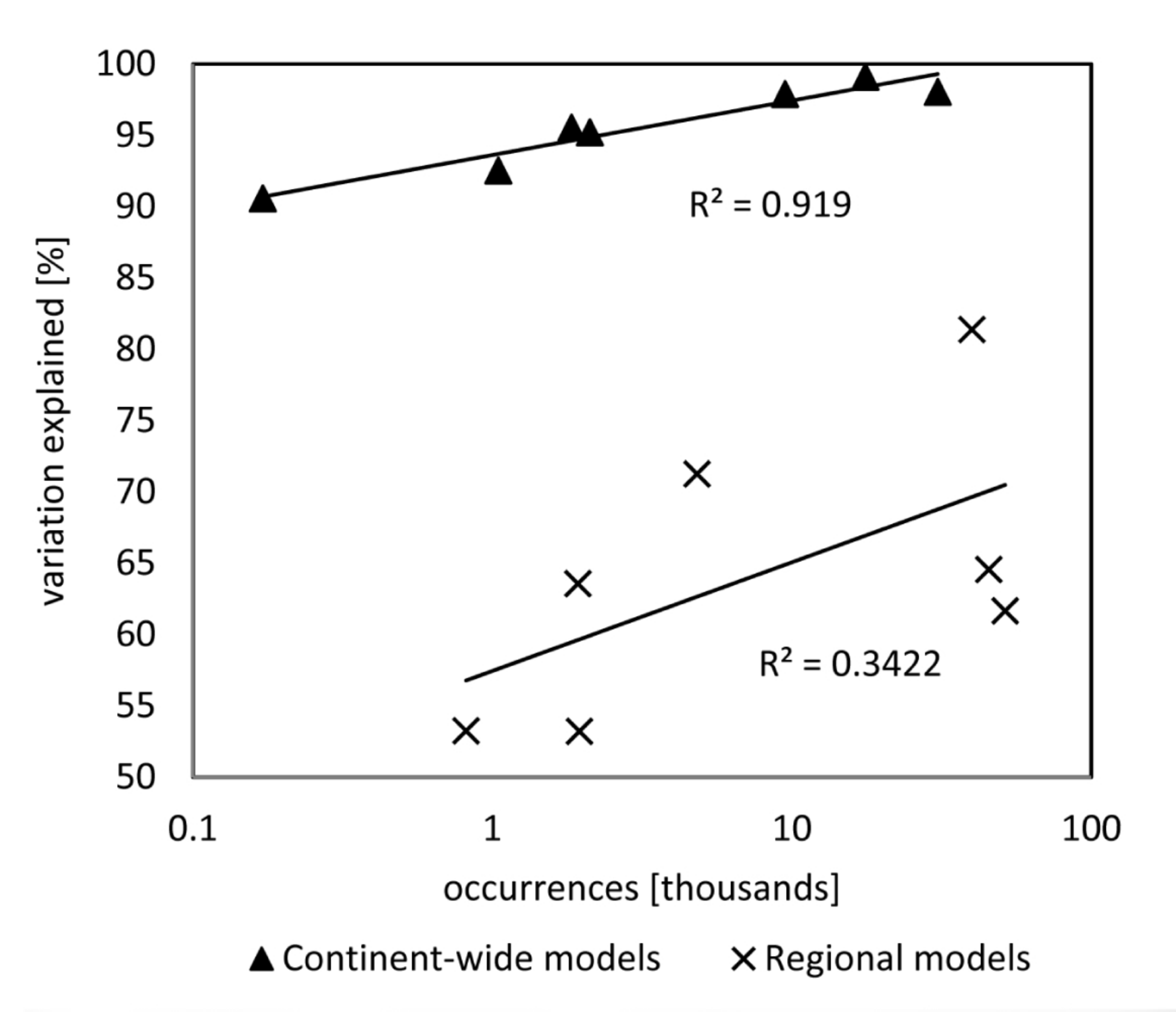
3.1. Model Training Data, Model Performance, and Accuracy

Species distribution models were trained to elaborate the ecological niche of the target species by combining explanatory variables and occurrence data. Occurrence data across Europe cover a much wider climatic range (Figure 2a) for all species than the climatic spectrum of the TBR. However, the climate range also varies among species, with P. nigra and U. leavis revealing the smallest climatic amplitudes. The relocation of the TBR’s climatic envelope indicates that most of the species currently present in the area of the TBR are likely to be forced out from their macro climatic niche due to climate change.
Occurrence data for the regional models demonstrate the relationship with riparian habitats for P. nigra and U. leavis occurring only in close proximity to rivers, not exceeding a 1–3 km horizontal distance and a 10–20 m altitudinal difference. The other species are less bound to the immediate river and occur also at larger distances from the river or at higher altitudes (Figure 2b).
Overall, the variation explained by the continent-wide models ranged from 91% to 99%, with highest values for F. excelsior (99.1%) and Q. robur (98.0%) and the lowest values for F. angustifolia (92.5%) and U. laevis (90.6%). The variation explained by the regional models ranged between 53% and 81%, with F. excelsior (81.4%) showing again the best performance and U. minor (53.5%) and Q. robur (53.2%) showing the weakest. In both datasets, an increasing number of occurrences resulted in a higher share of variation being explained (Figure A1).
The accuracies of the regional models were slightly lower compared to the continent-wide models. The specificity and sensitivity of the regional models ranged from 0.89 to 0.95, whereas the continent-wide models ranged from 0.98 to 1.00. The true skill statistic (TSS) of the regional models ranged from 0.79 to 0.91, whereas it varied from 0.99 to 1.00 for the continent-wide models. For the regional models, the accuracy for species such as A. glutinosa and the Q. robur was slightly lower compared to other species. In case of the continent-wide models, the accuracy between the species does not differ significantly (Table 1).

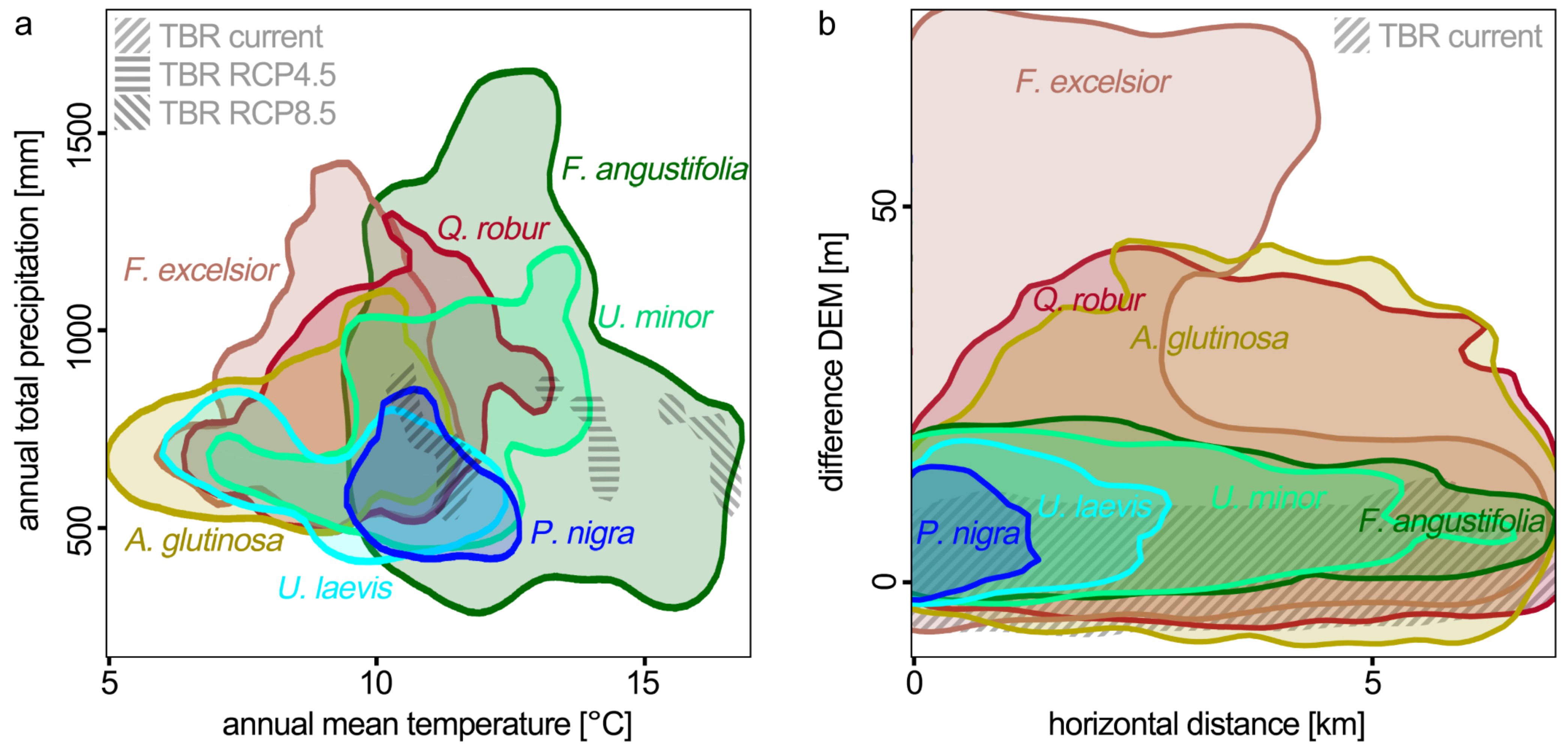
3.2. Drivers for Tree Species Distribution

Across the seven continental models, the most important variable (InMSE ± SD) was the maximum autumn temperature (98.5% ± 39.5%). It was selected for four species and explained up to 68% of the observed variation. In addition, the predictors continentality (25.3% ± 3.5%), annual precipitation (24.4% ± 3.3%), and mean summer precipitation (21.5% ± 13.5%) were significant predictors in four models. The summer heat-moisture index (52.8% ± 4.2%) and the maximum summer temperature (43.2% ± 1.7%) were suitable parameters for two species models. Other climatic predictor variables selected for only one species or with less importance (<21% on average) were found to be degree-days below 0 °C, mean coldest month temperature, longest frost-free period, mean spring precipitation, mean winter precipitation, annual heat-moisture index, and maximum spring temperature (Table A3).
Given the narrow climatic spectrum of the regional occurrence data set, climate variables explained only 21.8% ± 2.5% of the observed variation (34.5% ± 5.3% InMSE). In contrast, soil explained 28.7% ± 6.3% (44.4% ± 4.4% InMSE) and river proximity explained 13.6% ± 3.8% (21.0% ± 4.1% InMSE) of the variation.
The highest mean cumulative InMSE (±SD) was found for the soil variables (151.6% ± 55.4%), which included 18 potential predictors in total. The group of climate variables contained eight potential predictors, with a cumulated mean InMSE of 120.4% ± 62.1%, followed by the river variables (75.6% ± 42.7%).
The modeled species occurrence of F. excelsior and P. nigra were found to be mostly driven by the soil variables (41.3% and 32.2%), to which Q. robur occurrence was least sensitive (19.3%). The models for U. laevis and F. angustifolia were strongly affected by climate predictors. Compared to the other species’ models, P. nigra and F. excelsior were most strongly affected by the group of river predictors (20.3% and 18.2%), to which U. minor was least sensitive (9.0%, Table A4, Figure 3).

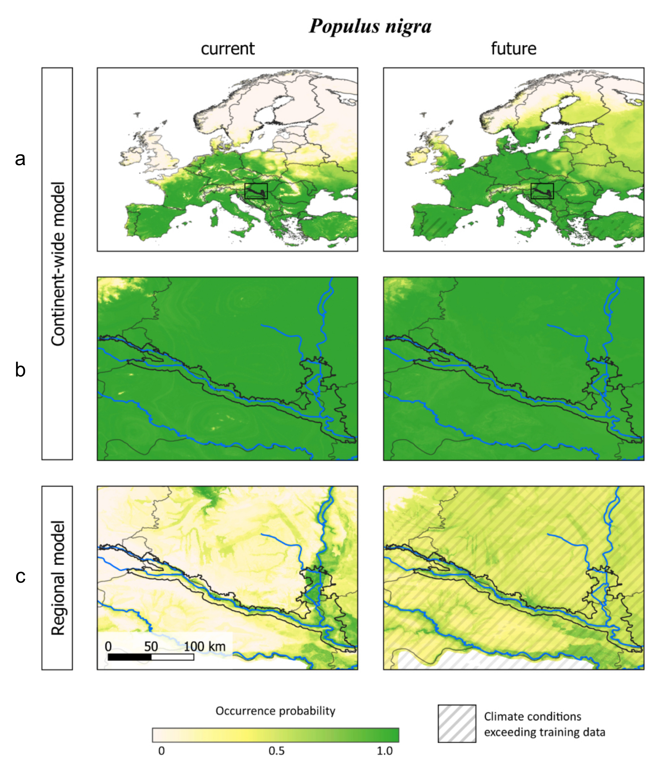
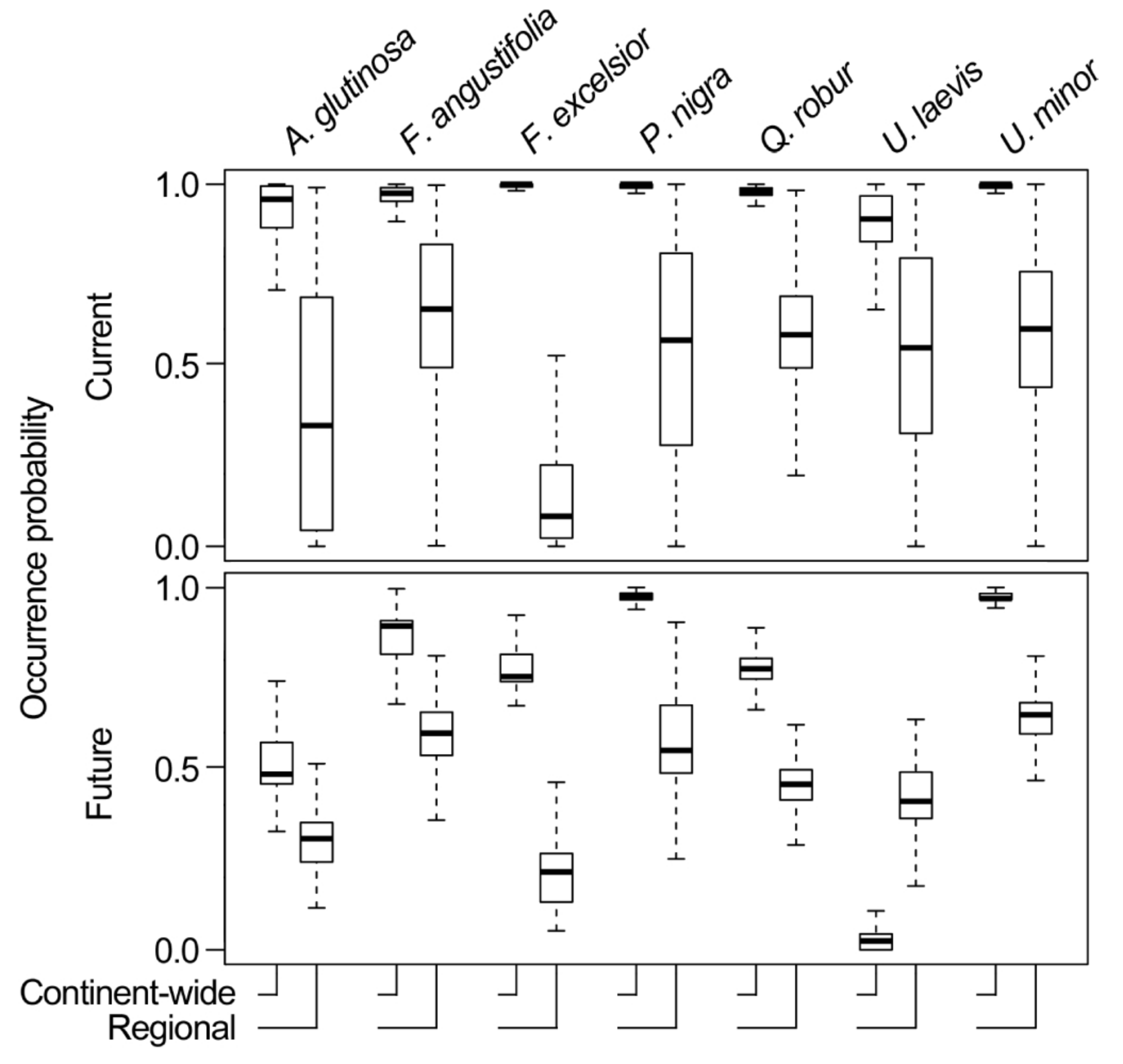
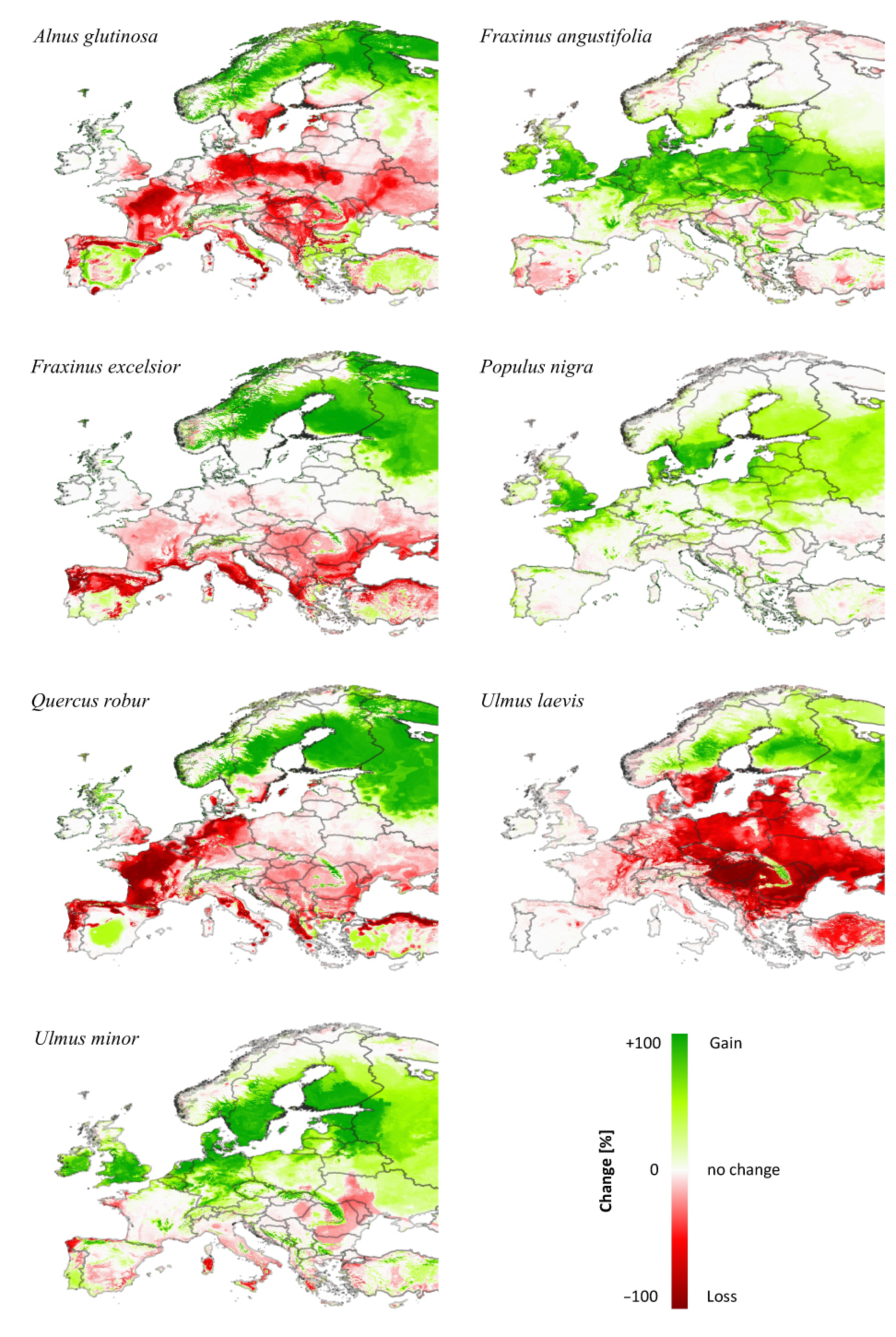
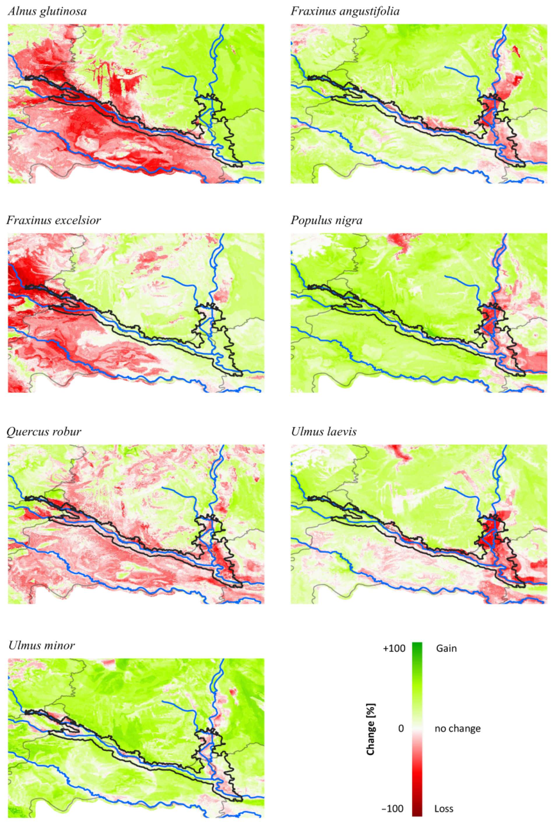
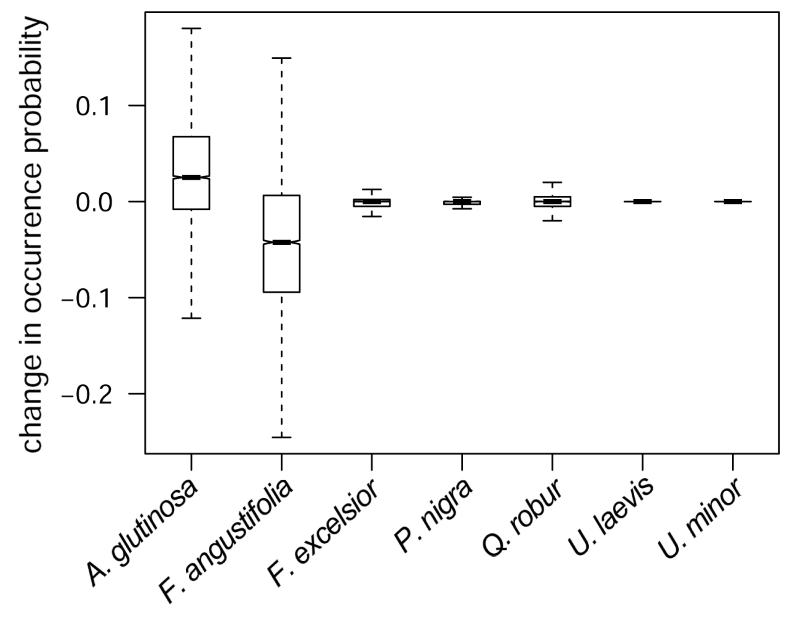
3.3. Comparing Model Type Predictions

Among the seven riparian forest tree species across Europe, six species are expected to expand their species range significantly under climate change. Increasing mean probabilities of occurrence show gains between 6% (A. glutinosa) and 27% (U. minor). The species P. nigra, F. angustifolia, and U. minor are expected to gain additional habitats in Western, Northern and Eastern Europe without larger losses in Southern Europe. F. angustifolia and Q. robur are expected to gain additional areas in north-eastern Europe, but at the same time, a loss of climatically suitable habitat in Southern and Western Europe was shown. In contrast, U. laevis is expected to lose significant parts of its current distribution in Central Europe and showed an overall decrease in its probability of occurrence of 9%. Its distribution range is expected to shift to north-eastern Europe and will be significantly smaller than the current one (Figure A2).
At the regional scale of the TBR, the continent-wide model generally predicted drastic future losses for all seven species. The regional models predicted a fine-scaled, more complex occurrence pattern. In contrast to the continent-wide models, the regional models were able to depict the regional core areas of tree distribution around major riparian landscapes by including a higher number of limiting environmental variables (Figure 4 and Electronic Supplementary Material S1). Future species distributions of both model types were more similar to each other than the current predictions. For six species, current and future probabilities of occurrence of the regional model were significantly lower than those of the continent-wide model. On the contrary, U. laevis displayed higher future probabilities in the regional compared to the continent-wide model (Figure 5). For U. leavis, the continent-wide model showed a strong decreasing trend across central and south-eastern Europe as well as within the Biosphere Reserve. The regional model confirmed this trend but still predicted future habitats along the rivers (Figure A3).
Patterns of the regional model for high future habitat suitability were in line with the continent-wide model but varied locally, as different predictors were used. Differences between the models were demonstrated by low or negative correlations for most species. Diffuse changes across the area resulted in low correlations between both models for many species (Table A5).

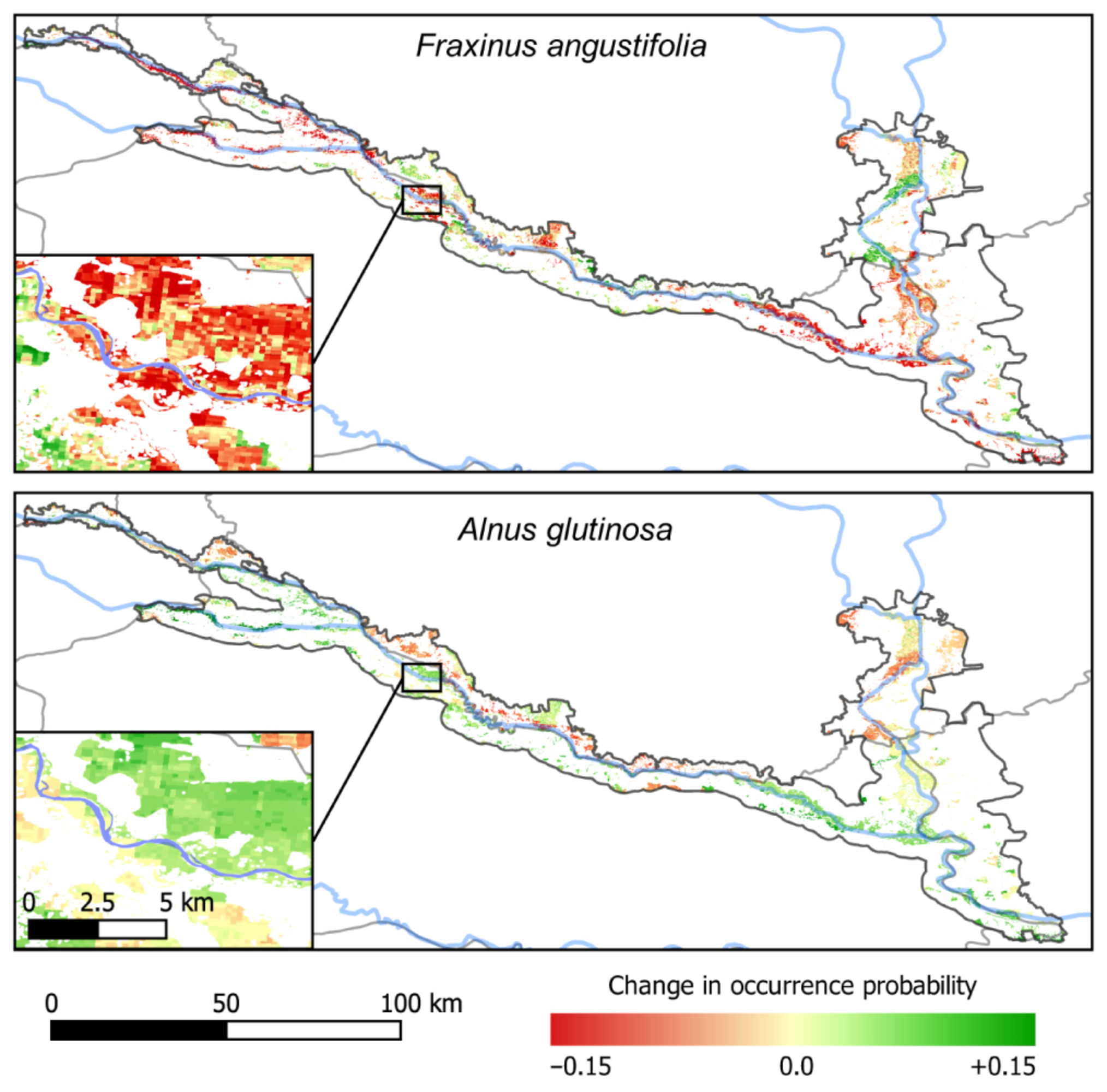
3.4. Predicted Co-Occurrence of Species

To investigate potential co-occurrence between the seven species, we estimated Pearson’s r correlation coefficient of occurrence probability for the current and future scenarios (Table A6). The range was −0.64 to 0.80. Applying a minimum threshold of 0.2 for the correlations, three groups of spatially associated tree species were derived: (I) F. angustifolia, P. nigra, U. laevis, and U. minor; (II) A. glutinosa, and F. excelsior; and (III) F. angustifolia, Q. robur, and U. minor. Under expected future conditions, the correlations of group (III) decreased below the threshold and instead two new groups evolved: (IIIa) A. glutinosa, F. angustifolia, and Q. robur; and (IIIb) A. glutinosa, and Q. robur. Changes in habitat suitability will unbalance the competition and are likely to affect the future mixture and functioning of forest stands.

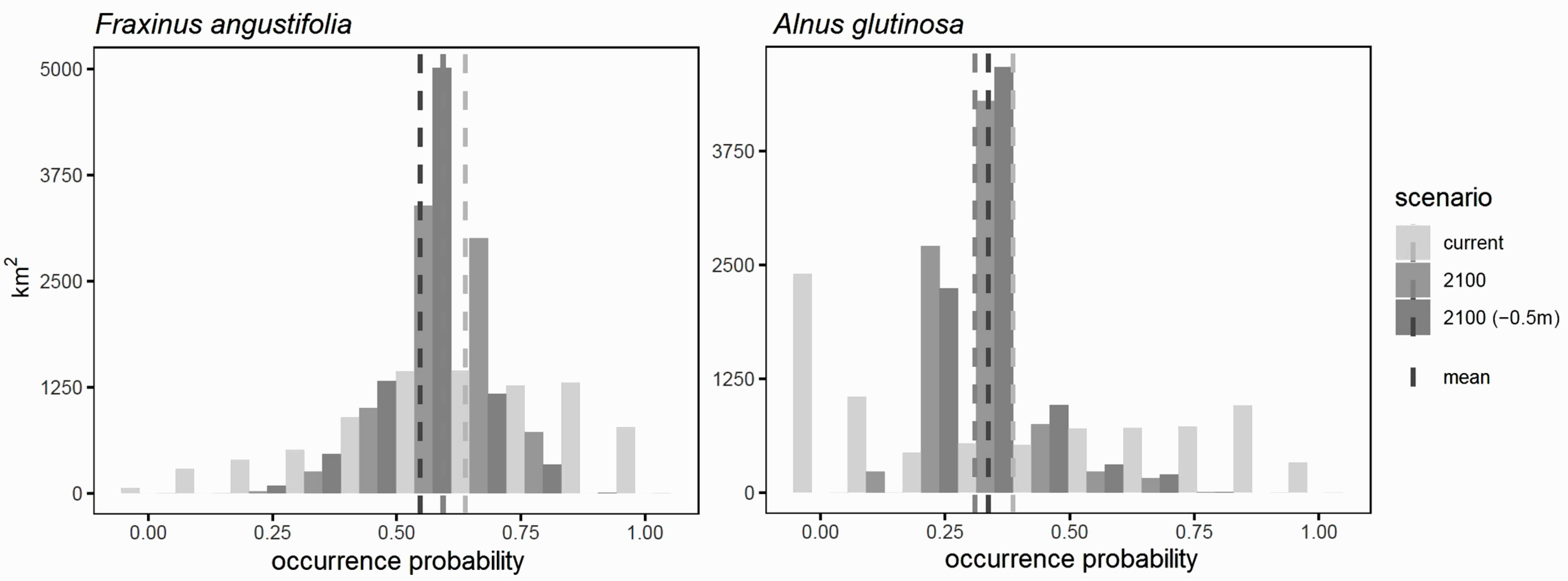
3.5. Consequences of River Deepening for Habitat Availability

To investigate the potential impact of river deepening on the future tree species occurrence, we tested the effects of river deepening by assuming a drop of 0.5 m throughout the study area. Despite the importance of the variable elevation difference to rivers for all species, only two tree species were significantly affected in occurrence probability distribution for the TBR in the models. The habitat of F. angustifolia was found to decrease by 5% occurrence probability on average and by 6% for the third quartile, which better covers the actual distribution. This may add to the decreasing occurrence probability induced by climate change. For the mean occurrence probability, the effect is similar to 102% of the magnitude of climate change until 2100 and for the third quartile to 36%. A. glutinosa showed the opposite trend. By applying the changed elevation differences, the average occurrence probability within the TBR increased by 3% and mitigated the predicted negative trend of climate change (Figure A4 and Figure A5). The predicted shifts are visible in the spatial pattern (Figure 6). These changes in occurrence probabilities are strongly site-dependent, but the observed trends of both species are also valid across the five countries.

4. Discussion

4.1. Consequences for Managing Riparian Forests of the TBR

Climate change is likely to force the currently present species out of their macro climatic niche. Our regional models showed a decrease in occurrence probability within the TBR for five of the seven species, whereas F. excelsior and U. minor could benefit. Paradoxically, these two species are already heavily threatened by severe diseases: F. excelsior by ash dieback, which is caused by the fungal species Hymenoscyphus fraxineus [87], and U. minor by Dutch elm disease, which is caused by the tubular fungus Ophiostoma novo-ulmi [88]. Overall, our results are in good agreement with studies analyzing the velocity of climate change, which showed that south-eastern European lowlands face among the highest velocity climate change across the continent [89,90] and a European-wide analysis of winner and loser species in conservation areas showed that our study region contains a high share of loser species in expected climate change [91].
The expected decreases in habitat suitability will not only impact the (potential) habitats of native plants, but can be expected to facilitate in particular a further spread of non-native plants [92,93,94]. This is because riparian forest development is strongly driven by regular flooding regimes [95], which drive small-scaled mortality with subsequent canopy gaps and irregular light regimes [96]. Additionally, river networks are essential vectors [97] and many non-native tree species are typical wetland species of riverine environments in their country of origin. Stimulated by these conditions, and in interaction with the prevailing propagule pressure, alien trees can be established [98]. Therefore, riparian forests have already developed as hotspots for this group [99,100]. With the (ongoing) dieback of trees or the disappearance of certain tree species, canopy gaps will become more frequent and environmental niches will become unoccupied, thereby further increasing susceptibility to invasion by non-natives.
To avoid a loss of forest functions, forest and conservation management needs to (i) evaluate the species’ potential to adapt to the changing environment, (ii) evaluate the artificial transfer of forest reproductive material from matching locations to speed up adaptation processes and reduce adaptation lags [101], (iii) rely on the potential of the other remaining native tree species to fill ecological gaps, or (iv) fill empty niches by means of assisted migration with new tree species which have desired characteristics. All passive measures raise the risk of uncontrolled penetration by tree species of an invasive character. Conservation management is faced with a decision between accepting such dynamics or counteracting them in advance or ex post facto. There have been positive and negative experiences with the active introduction of non-native tree species to riparian forests, such as Platanus orientalis, Juglans nigra, and Robinia pseudoacacia, as well as several non-native Populus species and their hybrids [102,103].
In contrast to our expectations, the deepening of rivers affected only two species considerably. We conclude that the models may be not sensitive enough to elevation modifications and highlight that soil parameters connected to water supply have not been modified. The periodic flooding favors riparian species adapted to such disturbances. However, it can be assumed that the models did not explicitly consider the suppression of riparian river dynamics, for instance by channel modifications or flood prevention dams, which can influence habitat suitability negatively.

4.2. Comparison of the Model Results and Predictor Importance with Other Studies

Our approach for the regional models targeted an optimal grain size as a trade-off between the necessity to describe riparian influences and the resolution of a forest stand level and model efficiency. The more realistic regional models generally explained less variation than the continent-wide models, in good agreement with previous studies [104,105].
The comparison of our future occurrence maps to existing SDM predictions was limited to the continent-wide model and a few species, as our target species are rarely investigated. Regarding Q. robur, very similar future distribution patterns were discovered by Schueler et al. [90] and Dyderski et al. [2]. Discrepancies were especially found in the southern European range, where our predictions indicate potential occurrences in the continental subtropical climates. Furthermore, a similar trend but with a more sensitive distribution pattern was predicted for the period 2061–2090 by Buras and Menzel [49], applying the same RCP scenarios. For F. excelsior, our prediction is comparable to Dyderski et al. [2] in RCP 8.5 across the full range, except in parts of the Scandinavian peninsula, where our occurrence probability prediction was significantly lower. Thurm et al. [51] modeled the future distribution of U. laevis using climate and soil data and found a significant increase in its distribution area to 227% across Europe up to 2070 by applying RCP 8.5. In contrast, our continent-wide model prediction of the same climate change scenario indicated a distribution change to the north-east, with major losses in Europe up to 2100. Encompassing further soil and river variables, our regional model also predicted much lower occurrence probabilities for the current and future climates. Reasons for these differences are related to a different variable set, differing origins of the input data, or the assumptions made in the modeling approach. More generally, such differences highlight the need for better datasets of species occurrences and environmental drivers for rare tree species with specific habitat requirements.
Regarding the importance of the model predictors in our regional models, soil variables were found to be the most important group, in agreement with other studies applying such environmental predictors [56,57,59]. Climate and river distance variables were found to have a lower impact. Velazco et al. [58] showed that on a worldwide scale the use of additional edaphic predictors increased SDM performance, and we concluded that soil variables could also increase the predictive ability of continent-wide models if aimed at this objective. Similarly to our regional model, a model for a mountainous landscape in Switzerland including climate and soil variables [59] found soil variables to be the most important for F. excelsior. By contrast, climatic variables for Q. robur were only slightly more important in our model, whereas they clearly dominated in the study by Walthert and Meier [59]. This is likely due to the different regional characteristics—Walthert and Meier [59] studied the distribution of Q. robur in Switzerland, including the cold-induced edge of its distribution, whereas our study analyzed oak populations close to the warm end of their current potential distribution. The variables of degree days were considered most important within the climatic group in the regional models for F. angustifolia, P. nigra, Q. robur, and U. laevis in contrast to the continent-wide model, where the maximum temperatures were the most important for six of the seven species. The importance of degree days was already highlighted by Dubuis et al. [106], who showed this predictor to be the most important in their models applying soil and climate data at a regional scale in Switzerland.

4.3. Data and Model Constraints

The distribution of tree species has been studied and modeled throughout the last decades [107,108,109], often focusing on zonal climax forest communities reflecting regional climate norms [59,109]. However, due to the limited availability of specific environmental predictors for their occurrence, riparian species have not been investigated to our knowledge.
Our models were based on two types of tree occurrence data sets and different environmental data, and they featured different grain sizes. The employed EU-Forest occurrence dataset includes the edges of continent-wide tree species distribution and is widely accepted for SDMs, but is limited to a resolution of 1 km. In contrast, collecting precise occurrence data as used in the regional model can be time- and cost-intensive, but strongly contributes to more realistic fine-scaled predictions. The applied bioclimatic data were similar for both developed model types. Superior to other available climate datasets, it provides 1 km spatial resolution (interpolated). The European Soil Database v2-Raster Library [79], with a spatial resolution of 1 km, matches the bioclimatic data, but cannot compete in accuracy with the other employed data and might limit the accuracy of our models. Forest communities can change within a few meters laterally or few decimeters vertically to the rivers, and with the regard to the precision of the occurrence, river, and elevation data, more accurate models could be built. Additionally, geographic proximity to a river increases the probability of flood events, with a limiting effect for many tree species. Consequently, our two river variables demonstrated an explanatory power nearly equivalent to bioclimatic variables over all investigated species. As the interaction between river level change and soil (water) parameters is complex, we did not modify the latter for our river level change scenario. In our models we could not differentiate between active and former floodplains where flooding was restricted by structural measures, as the applied systems for the delineation are different across the five countries and river systems. Alternatively to basic DEMs, flood area models could provide more reliable predictors for modeling riparian tree species distribution. In our case, such data were not available for the extent of our study area as it covered five countries and three river systems. Despite the influence of rivers on soil parameters and artificial limitation of flood areas, including river data enabled us to increase the resolution and accuracy.
For species distribution modeling, it is also important to be aware that the locations and species compositions of forests in Europe strongly reflect the results of anthropogenic influences [110,111,112]. Much of Europe’s forest area has undergone a significant transformation throughout history. In Hungary, for example, the age structure of forests reflects the growing periods of pines and poplars until the last “era of black locust”. Therefore, based on current distribution data, the natural distribution potential of tree species can only be partially reconstructed, especially in lowland areas. In SDMs, these limitations must be considered in order to interpret potential distributions. Furthermore, river levels have already changed significantly in the past and due to time lags in forest composition these changes might not be mirrored in the observed tree occurrences with which our model was trained. Therefore, a further change in river depth of 50 cm, as assumed in additional predictions of this study, might have greater consequences for habitat suitability than those expressed in our mapping.
We did not include any land cover information [2,60,61] besides the topographic river derivations, as we intended to predict occurrence probability independently from the current use of riparian zones to enable application for restoration projects. As an example of including land cover for areal habitat assessments, we hereby refer to Figure 6, where we cropped our results to forested areas. Although studies have shown the importance of differences in light regime between north- and south-facing slopes for species occurrence [62,108], we did not include this variable since our study area consisted of typical lowland river basins without considerable slopes.
In the field of ecology and the case of black-box methods used for predictions, a validation of the models not only statistically but also by existing ecological knowledge is important. Validating the predictions revealed limitations in the models’ behavior and indicated constraints based on the variable selection process. In the case of P. nigra, the model did not really find a variable that would negatively affect the distribution of the tree species as climate change progressed and the projections mainly indicate area gains. Similarly, we found constraints for the regional model of Q. robur, with future probability losses at the rivers and gains outside this area where distance as a predictor no longer had a significant effect, and the increase in degree-days and the increase in the annual heat-moisture index values became dominant and increased the probability. Thus, the predicted slight increase outside the vicinity of rivers should be treated with caution. In the Electronic Supplementary Material S2, we describe the functional relationship between the important predictors and predicted occurrence probabilities for both model types and all species, facilitating the correct interpretation of the predicted maps.

4.4. Practical Application of the Models

The continent-wide model easily assesses the climatic niche for the continent-wide population and can depict climate-change-driven modifications of occurrence probability on a continent-wide scale. With this model being limited to climate predictors, it is very sensitive to expected climate change. Thus, compared to the regional model, the predicted impact of climate change is higher and the resulting occurrence probability is in fact the bioclimatic suitability. Therefore, such continent-wide models might overestimate real occurrence changes but can be recommended for early warnings regarding climate change.
The precise occurrences applied in the regional model allowed us to model spatially complex patterns at a significantly smaller grain size. The proximity to the river could be efficiently used to understand the drivers for local variation in tree occurrence. Furthermore, the regional model focused on a subpopulation of the trees adapted to specific environmental conditions and does not capture the full populations’ environmental range. The future environment might be unsuitable for the local population but could potentially match the requirements of other (sub)populations. Therefore, predicted mismatches are not equal to a low occurrence probability for the species in general and do not necessarily exceed the population’s ecological amplitude. Derived ecological niches need to be seen in this context and are not spatially transferable [48,113]. In contrast, a general problem that increases with smaller geographic scale is that changing climate conditions are not encompassed by the training data. Nearly 60% of over 200 SDM studies reviewed by Porfirio [114] assessed climate change impacts at the regional scale and were potentially forced to extrapolate, whereas only 14% considered continent-wide scales. Our investigations highlight this problem, driven by serious climatic changes both in RCP 4.5 and RCP 8.5 scenarios, especially for the regional model. The predictions indicate major alterations in species distribution even without the extrapolation of trends in occurrence probability, and we assume that extrapolation would have further increased the magnitude of predicted changes.
Nevertheless, the complex spatial pattern that can be realized with regional models reaching down to stand level resolution, as well as the opportunity to precisely match the spatial extent to certain purposes or populations, predestines them to support decision-making by forest and conservation managers. Especially in terms of adapting to climate change, such realistic predictions are of increasing value. For the operative use, standard large-scale bioclimatic models alone are too coarse and frequently exclude relevant predictors. We recommend using multiple model predictions with different scales and various predictor groups [115] and to consider the uncertainties related to the underlying model assumptions [48] (pp. 126–127).

5. Conclusions

This study provides SDMs for seven major tree species in riparian forests to guide forest and conservation management in the five-country transboundary Biosphere Reserve Mura-Drava-Danube (TBR). Climate change is likely to force present foundation tree species out from their macro climatic niches. A. glutinosa, Q. robur, and U. laevis are expected to substantially suffer from changing climate conditions, whereas F. excelsior and U. minor could potentially benefit by the end of this century. The results of this study can support decision-making at a local level such as in tree species selection [46], prioritization of conservation and restoration activities [48,116,117], and raising awareness regarding the impacts of climate change [2,50,53].

Supplementary Materials

The following are available online at https://www.mdpi.com/1999-4907/12/3/330/s1: Electronic Supplementary Material S1: Occurrence probability maps; Electronic Supplementary Material S2: Evaluation of tree species models.

Author Contributions

D.C., M.S., and S.S. developed the methodology; M.S., M.L., A.R., G.I., A.K., and D.S. prepared the data; M.S. performed the statistical analyses and prepared the graphics; M.S. wrote the initial manuscript and led the joint finalization by all authors; S.S. and H.V. supervised the work; S.S. acquired the funding. All authors have read and agreed to the published version of the manuscript.

Funding

This research was supported by the INTERREG Danube program (Project REFOCuS: Resilient Riparian Forest in the Mura-Drava-Danube Biosphere Reserve, DTP2-044-2.3).

Institutional Review Board Statement

Not applicable.

Informed Consent Statement

Not applicable.

Data Availability Statement

The data generated and presented in this study are available in Supplementary Material S1.

Acknowledgments

For providing occurrence data we thank the Public Company of Vojvodinašume (RS), the Hungarian National Land Centre (HU), and the Slovenia Forest Service (SL). We are grateful for the helpful comments of the anonymous referees.

Conflicts of Interest

The authors declare no conflict of interest.

Appendix A

Table A1. Number of employed occurrences for developing the two types of models of the seven selected target species. The continent-wide models were trained with occurrences and climate data only, whereas the regional models were based on precise occurrences on a smaller spatial scale and a larger environmental dataset of climate, river, and soil variables.
Model TypeAlnus glutinosaFraxinus angustifoliaFraxinus excelsiorPopulus nigraQuercus roburUlmus laevisUlmus minor
continent-wide9488104617,596211530,7001711836
regional39,918482145,445192951,5398161952
Table A2. List of variables used in the variable selection process for the continent-wide and the regional models.
Continent-wide and regional modelAHMAnnual heat:moisture index
bFFPBeginning of FFP
DDabove18Degree-days above 18 °C
DDabove5Degree-days above 5 °C
DDbelow0Degree-days below 0 °C
DDbelow18Degree-days below 18 °C
eFFPEnds of FFP
EMTExtreme minimum temperature
FFPLongest frost-free period
MAPAnnual total precipitation
MATAnnual mean temperature
MCMTMean coldest month temperature
MWMTMean warmest month temperature
NFFDNumber of frost-free days
PPT_atMean autumn precipitation
PPT_smMean summer precipitation
PPT_spMean spring precipitation
PPT_wtMean winter precipitation
SHMSummer heat:moisture index
Tave_atMean autumn temperature
Tave_smMean summer temperature
Tave_spMean spring temperature
Tave_wtMean winter temperature
TDContinentality
Tmax_atMaximum autumn temperature
Tmax_smMaximum summer temperature
Tmax_spMaximum spring temperature
Tmax_wtMaximum winter temperature
Tmin_atMinimum autumn temperature
Tmin_smMinimum summer temperature
Tmin_spMinimum spring temperature
Tmin_wtMinimum winter temperature
Regional modelmin_direct_distHorizontal distance to the next water body (major rivers and inland water bodies)
diff_demElevation difference between site and next river. Calculated from a 25 × 25 m Digital Elevation Model
awc_subSubsoil available water capacity
awc_topTopsoil available water capacity
bs_subBase saturation of the subsoil
bs_topBase saturation of the topsoil
cec_subSubsoil cation exchange capacity
cec_topTopsoil cation exchange capacity
dghDepth to a gleyed horizon
dimpDepth to an impermeable layer
drDepth to rock
eawc_subSubsoil easily available water capacity
eawc_topTopsoil easily available water capacity
hgHydrogeological class
oc_topTopsoil organic carbon content
pd_subSubsoil packing density
pd_topTopsoil packing density
peatPeat
pmhParent material hydrogeological type
str_subSubsoil structure
str_topTopsoil structure
textDominant surface textural class (completed from dominant STU)
Figure A1. Explained variations by 14 developed species distribution models of two types in relation to the number of occurrences. The continent-wide models were trained and tested with generalized occurrences and climate data only, whereas the regional models were based on precise occurrences on a smaller spatial scale and different environmental data comprising climate, river, and soil variables.
Forests 12 00330 g0a1
Table A3. Number of employed occurrences in the continent-wide models, the models’ variation explained, selected predictors, and the corresponding percentage increase in mean square error (InMSE) when the variable is dropped from the models for the seven selected target species.
SpeciesOccurrencesVariation Explained (%)Explanatory Variables: InMSE
Alnus glutinosa948897.89Tmax_at: 76.9SHM: 48.4MAP: 27.1TD: 24.1-
Fraxinus angustifolia104692.53Tmax_at: 42.5TD: 25.3MAP: 23PPT_wt: 15.2-
Fraxinus excelsior17,59699.10Tmax_at: 144.5SHM: 56.8PPT_sp: 9.8--
Populus nigra211595.21Tmax_sm: 44.9DDbelow0: 21PPT_sp: 20.1PPT_sm: 14.0-
Quercus robur30,70098.04Tmax_at: 122.1PPT_sm: 44.6TD: 30.6MAP: 27.9-
Ulmus laevis17190.57MCMT: 17.7PPT_wt: 12.7AHM: 12.7Tmax_sp: 12.3PPT_sm: 10.9
Ulmus minor183695.54Tmax_sm: 41.5TD: 20.6MAP: 19.5PPT_sm: 16.7FFP: 16.0
Table A4. Number of employed occurrences in the regional models, the models’ variation explained, selected predictors, and the corresponding percentage increase in mean square error (InMSE) when the variable is dropped from the models for the seven selected target species.
SpeciesOccurrencesVariation Explained (%)Explanatory Variables: InMSE
Alnus glutinosa39,91861.66diff_dem: 78; AHM_199110_1km: 61.8; DDbelow0_199110_1km: 49.4; DDabove5_199110_1km: 42.2; dr: 18.2; hg: 17.7; pmh: 17.4; awc_sub: 15.5; cec_sub: 14; bs_top: 13.5; awc_top: 12.1; oc_top: 11.5; pd_top: 10.6; bs_sub: 10.5; str_top: 10.5; text: 10.1; cec_top: 9.3; pd_sub: 8.9; dgh: 6.9; peat: 6.2;
Fraxinus angustifolia482164.56DDbelow0_199110_1km: 39.5; AHM_199110_1km: 37.6; min_direct_dist: 25.8; DDabove5_199110_1km: 25.6; diff_dem: 23.4; hg: 15.9; awc_sub: 11.6; cec_sub: 10.5; cec_top: 9.8; awc_top: 9.7; text: 9.7; dr: 9.4; dgh: 8.7; str_top: 8.3; bs_top: 7.4; pd_sub: 7.2; pd_top: 7.1; dimp: 5.3; str_top: 4.2; peat: 4.1;
Fraxinus excelsior45,44581.38AHM_199110_1km: 57.0; min_direct_dist: 50.1; DDbelow18_199110_1km: 42.8; diff_dem: 32.5; awc_sub: 16.9; cec_sub: 16.4; cec_top: 16; hg: 13.4; text: 12.2; pd_sub: 11.9; pmh: 11.4; dr: 11.2; bs_top: 11.2; awc_top: 10.9; bs_sub: 10.9; dgh: 10; oc_top: 8.9; str_top: 8.7; pd_top: 7; str_top: 6.7; peat: 3.7;
Populus nigra192971.26min_direct_dist: 50.5; diff_dem: 26.5; DDabove18_199110_1km: 25.2; DDbelow0_199110_1km: 24.7; AHM_199110_1km: 21.8; pmh: 10.9; hg: 10.4; cec_top: 10.4; text: 9.7; str_top: 8.9; pd_sub: 7.6; bs_sub: 7.1; awc_top: 7; dr: 6.8; bs_top: 6.8; pd_top: 6.7; cec_sub: 6.6; oc_top: 5.9; dgh: 5.7; dimp: 5.6; str_top: 3.4; peat: 3.1;
Quercus robur51,53953.21DDabove5_199110_1km: 89.2; EMT_199110_1km: 88.9; min_direct_dist: 87.1; diff_dem: 82.4; AHM_199110_1km: 79.5; awc_sub: 20.5; dr: 19.4; str_top: 17.3; cec_sub: 17.2; text: 17; hg: 16.2; bs_top: 15.9; awc_top: 15.6; bs_sub: 15.5; pmh: 15.4; oc_top: 15.2; cec_top: 13.3; dgh: 12.3; pd_top: 11.3; str_top: 9; pd_sub: 6.8; peat: 4.4;
Ulmus laevis81663.57min_direct_dist: 20.7; DDbelow0_199110_1km: 20.2; DDabove18_199110_1km: 19.4; AHM_199110_1km: 13; FFP_199110_1km: 10.2; diff_dem: 7.3; hg: 5.8; text: 5.4; dr: 5.2; awc_sub: 4.7; oc_top: 4.5; awc_top: 4.4; cec_sub: 3.8; pmh: 3.4; cec_top: 3.4; bs_top: 3.1; str_top: 3.1; dimp: 2.9; pd_top: 2.8; dgh: 2.8; pd_sub: 2.2; bs_sub: 2.1; str_top: 1.2;
Ulmus minor195253.25MAP_199110_1km: 38.5; DDabove5_199110_1km: 29.8; DDbelow0_199110_1km: 26.9; diff_dem: 22.6; min_direct_dist: 22.4; hg: 10.7; dr: 10.7; pmh: 10; awc_sub: 9.7; bs_top: 8.9; bs_sub: 8.7; str_top: 8.5; text: 8.2; oc_top: 7.9; pd_top: 7.3; cec_top: 6.9; cec_sub: 6.7; pd_sub: 6.4; awc_top: 5.5; dgh: 4.9; str_top: 4.2; peat: 0.9;
Figure A2. Absolute gains and losses in occurrence probability between current and future predictions of the continent-wide model (RCP 8.5, 2081–2100).
Forests 12 00330 g0a2
Figure A3. Absolute gains and losses in occurrence probability between current and future predictions of the regional model (RCP 8.5, 2081–2100).
Forests 12 00330 g0a3
Table A5. Correlation coefficients between the continent-wide models and the regional models for (a) current predictions, (b) future predictions, and (c) differences between current and future predictions calculated for 6000 random points within the transboundary Biosphere Reserve Mura-Drava-Danube.
CorrelationAlnus glutinosaFraxinus angustifoliaFraxinus excelsiorPopulus nigraQuercus roburUlmus laevisUlmus minor
(a) Current−0.170.71−0.440.070.27−0.45−0.04
(b) Future0.29−0.33−0.03−0.12−0.180.030.08
(c) Change−0.020.640.540.100.140.39−0.15
Table A6. Pearson’s r correlation coefficient for the predicted occurrence probabilities between the seven tree species at 6000 randomly distributed points across the transboundary Biosphere Reserve for the current and future scenarios of the regional model.
Forests 12 00330 i001
Figure A4. Change in future occurrence probability for all seven riparian tree species estimated with the regional model between a scenario with current river levels and a scenario with deepened river soles by 0.5 m.
Forests 12 00330 g0a4
Figure A5. Frequency distribution across the Mura-Drava-Danube Biosphere Reserve for current, future, and future occurrence probability with 0.5 m river deepening, predicted by the regional models for Fraxinus angustifolia and Alnus glutinosa.
Forests 12 00330 g0a5

References

  1. Jones, K.R.; Venter, O.; Fuller, R.A.; Allan, J.R.; Maxwell, S.L.; Negret, P.J.; Watson, J.E.M. One-third of global protected land is under intense human pressure. Science 2018, 360, 788–791. [Google Scholar] [CrossRef] [PubMed] [Green Version]
  2. Dyderski, M.K.; Paź, S.; Frelich, L.E.; Jagodziński, A.M. How much does climate change threaten European forest tree species distributions? Glob. Chang. Biol. 2018, 24, 1150–1163. [Google Scholar] [CrossRef] [PubMed]
  3. Bentz, B.J.; Régnière, J.; Fettig, C.J.; Hansen, E.M.; Hayes, J.L.; Hicke, J.A.; Kelsey, R.G.; Negrón, J.F.; Seybold, S.J. Climate change and bark beetles of the Western United States and Canada: Direct and indirect effects. Bioscience 2010, 60, 602–613. [Google Scholar] [CrossRef]
  4. Jönsson, A.M.; Appelberg, G.; Harding, S.; Bärring, L. Spatio-temporal impact of climate change on the activity and voltinism of the spruce bark beetle, Ips typographus. Glob. Chang. Biol. 2009, 15, 486–499. [Google Scholar] [CrossRef]
  5. Beniston, M.; Stephenson, D.B.; Christensen, O.B.; Ferro, C.A.T.; Frei, C.; Goyette, S.; Halsnaes, K.; Holt, T.; Jylhä, K.; Koffi, B.; et al. Future extreme events in European climate: An exploration of regional climate model projections. Clim. Chang. 2007. [Google Scholar] [CrossRef] [Green Version]
  6. Seidl, R.; Thom, D.; Kautz, M.; Martin-Benito, D.; Peltoniemi, M.; Vacchiano, G.; Wild, J.; Ascoli, D.; Petr, M.; Honkaniemi, J.; et al. Forest disturbances under climate change. Nat. Clim. Chang. 2017, 7, 395–402. [Google Scholar] [CrossRef] [Green Version]
  7. Dubrovský, M.; Hayes, M.; Duce, P.; Trnka, M.; Svoboda, M.; Zara, P. Multi-GCM projections of future drought and climate variability indicators for the Mediterranean region. Reg. Environ. Chang. 2014, 14, 1907–1919. [Google Scholar] [CrossRef]
  8. Hanel, M.; Rakovec, O.; Markonis, Y.; Máca, P.; Samaniego, L.; Kyselý, J.; Kumar, R. Revisiting the recent European droughts from a long-term perspective. Sci. Rep. 2018, 8, 9499. [Google Scholar] [CrossRef] [PubMed]
  9. Arnell, N.W.; Gosling, S.N. The impacts of climate change on river flood risk at the global scale. Clim. Chang. 2016, 134, 387–401. [Google Scholar] [CrossRef] [Green Version]
  10. Dottori, F.; Szewczyk, W.; Ciscar, J.C.; Zhao, F.; Alfieri, L.; Hirabayashi, Y.; Bianchi, A.; Mongelli, I.; Frieler, K.; Betts, R.A.; et al. Increased human and economic losses from river flooding with anthropogenic warming. Nat. Clim. Chang. 2018, 8, 781–786. [Google Scholar] [CrossRef]
  11. Winsemius, H.C.; Aerts, J.C.J.H.; Van Beek, L.P.H.; Bierkens, M.F.P.; Bouwman, A.; Jongman, B.; Kwadijk, J.C.J.; Ligtvoet, W.; Lucas, P.L.; Van Vuuren, D.P.; et al. Global drivers of future river flood risk. Nat. Clim. Chang. 2016, 6, 381–385. [Google Scholar] [CrossRef]
  12. Mikulová, K.; Jarolímek, I.; Šibík, J.; Bacigál, T.; Šibíková, M. Long-Term changes of softwood floodplain forests—Did the disappearance of wet vegetation accelerate the invasion process? Forests 2020, 11, 1218. [Google Scholar] [CrossRef]
  13. Hulme, P.E. Trade, transport and trouble: Managing invasive species pathways in an era of globalization. J. Appl. Ecol. 2009, 46, 10–18. [Google Scholar] [CrossRef]
  14. Meyerson, L.A.; Mooney, H.A. Invasive alien species in an era of globalization. Front. Ecol. Environ. 2007, 5, 199–208. [Google Scholar] [CrossRef]
  15. Boyd, I.L.; Freer-Smith, P.H.; Gilligan, C.A.; Godfray, H.C.J. The consequence of tree pests and diseases for ecosystem services. Science 2013, 342. [Google Scholar] [CrossRef] [PubMed]
  16. Hansen, E.M. Alien forest pathogens: Phytophthora species are changing world forests. Boreal Environ. Res. 2008, 13, 33–41. [Google Scholar]
  17. Allard, G.; Sigaud, P. Alien Invasive Species: Impacts on Forests and Forestry—A Review. Available online: http://www.fao.org/3/j6854e/J6854E06.htm (accessed on 30 March 2020).
  18. Nisbet, D.; Kreutzweiser, D.; Sibley, P.; Scarr, T. Ecological risks posed by emerald ash borer to riparian forest habitats: A review and problem formulation with management implications. For. Ecol. Manag. 2015, 358, 165–173. [Google Scholar] [CrossRef]
  19. Nadal-Sala, D.; Hartig, F.; Gracia, C.A.; Sabaté, S. Global warming likely to enhance black locust (Robinia pseudoacacia L.) growth in a Mediterranean riparian forest. For. Ecol. Manag. 2019, 449, 117448. [Google Scholar] [CrossRef]
  20. Tockner, K.; Stanford, J.A. Riverine flood plains: Present state and future trends. Environ. Conserv. 2002, 29, 308–330. [Google Scholar] [CrossRef] [Green Version]
  21. Nilsson, C.; Berggren, K. Alterations of Riparian Ecosystems Caused by River Regulation. Bioscience 2000, 50, 783. [Google Scholar] [CrossRef]
  22. Roder, G.; Sofia, G.; Wu, Z.; Tarolli, P. Assessment of Social Vulnerability to floods in the floodplain of northern Italy. Weather Clim. Soc. 2017, 9, 717–737. [Google Scholar] [CrossRef]
  23. Belletti, B.; Garcia de Leaniz, C.; Jones, J.; Bizzi, S.; Börger, L.; Segura, G.; Castelletti, A.; van de Bund, W.; Aarestrup, K.; Barry, J.; et al. More than one million barriers fragment Europe’s rivers. Nature 2020, 588, 436–441. [Google Scholar] [CrossRef] [PubMed]
  24. Bonacci, O.; Oskorǔ, D. The changes in the lower Drava River water level, discharge and suspended sediment regime. Environ. Earth Sci. 2010, 59, 1661–1670. [Google Scholar] [CrossRef]
  25. Bonacci, O.; Oskoruš, D. The influence of three Croatian hydroelectric power plants operation on the river Drava hydrological and sediment regime. Hydrol. Forecast. 2008. [Google Scholar]
  26. Globevnik, L.; Kaligaric, M. Hydrological changes of the Mura River in Slovenia, accompanied with habitat deterioration in riverine space. RMZ Mater. Geoenviron. 2005, 52, 45–49. [Google Scholar]
  27. Habersack, H. Wasserbau, Schifffahrt und Ökologie an der Donau–Pilotprojekt Bad Deutsch-Altenburg. Osterr. Wasser Und Abfallwirtschaft 2016, 68, 190–192. [Google Scholar] [CrossRef] [Green Version]
  28. Klimo, E.; Hager, H.; Matič, S.; Anič, I.; Kulhavý, J.; Nilsson, C.; Berggren, K. Floodplain Forests of the Temperate Zone of Europe; Brill Academic Publisher: Leiden, The Netherlands, 2008; ISBN 978-80-87154-16-8. [Google Scholar]
  29. Netsvetov, M.; Prokopuk, Y.; Puchałka, R.; Koprowski, M. River Regulation Causes Rapid Changes in Relationships Between Floodplain Oak Growth and Environmental Variables. Front. Plant. Sci. 2019, 10, 96. [Google Scholar] [CrossRef]
  30. Millennium Ecosystem Assessment. Ecosystems and Human Well-Being: Wetlands and Water Synthesis; Max Finlayson, C., Rebecca D’Cruz, N.D., Eds.; World Resources Institute: Washington, DC, USA, 2005. [Google Scholar]
  31. Leyer, I.; Mosner, E.; Lehmann, B. Managing floodplain-forest restoration in European river landscapes combining ecological and flood-protection issues. Ecol. Appl. 2012, 22, 240–249. [Google Scholar] [CrossRef] [PubMed]
  32. Sanjou, M.; Okamoto, T.; Nezu, I. Experimental study on fluid energy reduction through a flood protection forest. J. Flood Risk Manag. 2018, 11, e12339. [Google Scholar] [CrossRef] [Green Version]
  33. Kevey, B. Floodplain forests. In Springer Geography; Lóczy, D., Ed.; Springer: Cham, Switzerland, 2018; Volume PartF5, pp. 299–336. ISBN 978-3-319-92815-9. [Google Scholar]
  34. Schnitzler, A.; Hale, B.W.; Alsum, E. Biodiversity of floodplain forests in Europe and eastern North America: A comparative study of the Rhine and Mississippi Valleys. Biodivers. Conserv. 2005, 14, 97–117. [Google Scholar] [CrossRef]
  35. Sikorska, D.; Sikorski, P.; Archiciński, P.; Chormański, J.; Hopkins, R.J. You can’t see the woods for the trees: Invasive Acer negundo L. in Urban riparian forests harms biodiversity and limits recreation activity. Sustainability 2019, 11, 5838. [Google Scholar] [CrossRef] [Green Version]
  36. Cartisano, R.; Mattioli, W.; Corona, P.; Mugnozza, G.S.; Sabatti, M.; Ferrari, B.; Cimini, D.; Giuliarelli, D. Assessing and mapping biomass potential productivity from poplar-dominated riparian forests: A case study. Biomass Bioenergy 2013, 54, 293–302. [Google Scholar] [CrossRef] [Green Version]
  37. Seidl, R.; Klonner, G.; Rammer, W.; Essl, F.; Moreno, A.; Neumann, M.; Dullinger, S. Invasive alien pests threaten the carbon stored in Europe’s forests. Nat. Commun. 2018, 9, 1–10. [Google Scholar] [CrossRef]
  38. Dukes, J.S.; Pontius, J.; Orwig, D.; Garnas, J.R.; Rodgers, V.L.; Brazee, N.; Cooke, B.; Theoharides, K.A.; Stange, E.E.; Harrington, R.; et al. Responses of insect pests, pathogens, and invasive plant species to climate change in the forests of northeastern North America: What can we predict? This article is one of a selection of papers from NE Forests 2100: A Synthesis of Climate Change Impacts on Forests of the Northeastern US and Eastern Canada. Can. J. For. Res. 2009, 39, 231–248. [Google Scholar] [CrossRef]
  39. Charles, H.; Dukes, J.S. Impacts of Invasive Species on Ecosystem Services. In Biological Invasions; Springer: Berlin, Germany, 2007; pp. 293–310. [Google Scholar] [CrossRef]
  40. Vilà, M.; Hulme, P.E. Non-native Species, Ecosystem Services, and Human Well-Being. In Impact of Biological Invasions on Ecosystem Services; Springer: Cham, Switzerland, 2017; pp. 1–14. [Google Scholar]
  41. Ramsfield, T.D.; Bentz, B.J.; Faccoli, M.; Jactel, H.; Brockerhoff, E.G. Forest health in a changing world: Effects of globalization and climate change on forest insect and pathogen impacts. Forestry 2016. [Google Scholar] [CrossRef]
  42. Buras, A.; Sass-Klaassen, U.; Verbeek, I.; Copini, P. Provenance selection and site conditions determine growth performance of pedunculate oak. Dendrochronologia 2020, 61, 125705. [Google Scholar] [CrossRef]
  43. Havens, K.; Vitt, P.; Still, S.; Kramer, A.T.; Fant, J.B.; Schatz, K. Seed sourcing for restoration in an era of climate change. Nat. Areas J. 2015, 35, 122–133. [Google Scholar] [CrossRef]
  44. Konnert, M.; Fady, B.; Gömöry, D.; A’Hara, S.; Wolter, F.; Ducci, F.; Koskela, J.; Bozzano, M.; Maaten, T.; Kowalczyk, J. Use and Transfer of Forest Reproductive Material in Europe in the Context of Climate Change; European Forest Genetic Resources Programme (EUFORGEN); Bioversity International: Rome, Italy, 2015; ISBN 9789292550318. [Google Scholar]
  45. Falk, W.; Mellert, K.H. Species distribution models as a tool for forest management planning under climate change: Risk evaluation of Abies alba in Bavaria. J. Veg. Sci. 2011, 22, 621–634. [Google Scholar] [CrossRef]
  46. Bolte, A.; Ammer, C.; Löf, M.; Madsen, P.; Nabuurs, G.J.; Schall, P.; Spathelf, P.; Rock, J. Adaptive forest management in central Europe: Climate change impacts, strategies and integrative concept. Scand. J. For. Res. 2009, 24, 473–482. [Google Scholar] [CrossRef]
  47. Domisch, S.; Friedrichs, M.; Hein, T.; Borgwardt, F.; Wetzig, A.; Jähnig, S.C.; Langhans, S.D. Spatially explicit species distribution models: A missed opportunity in conservation planning? Divers. Distrib. 2019, 25, 758–769. [Google Scholar] [CrossRef]
  48. Riordan, E.C.; Montalvo, A.M.; Beyers, J.L. Using Species Distribution Models with Climate Change Scenarios to Aid Ecological Restoration Decisionmaking for Southern California Shrublands. Available online: https://www.fs.fed.us/psw/publications/documents/psw_rp270/psw_rp270.pdf (accessed on 7 November 2020).
  49. Buras, A.; Menzel, A. Projecting tree species composition changes of european forests for 2061–2090 under RCP 4.5 and RCP 8.5 scenarios. Front. Plant Sci. 2019, 9, 1–13. [Google Scholar] [CrossRef] [PubMed] [Green Version]
  50. Marchi, M.; Ducci, F. Some refinements on species distribution models using tree-level national forest inventories for supporting forest management and marginal forest population detection. iForest 2018, 11, 291–299. [Google Scholar] [CrossRef] [Green Version]
  51. Thurm, E.A.; Hernandez, L.; Baltensweiler, A.; Ayan, S.; Rasztovits, E.; Bielak, K.; Zlatanov, T.M.; Hladnik, D.; Balic, B.; Freudenschuss, A.; et al. Alternative tree species under climate warming in managed European forests. For. Ecol. Manag. 2018, 430, 485–497. [Google Scholar] [CrossRef]
  52. Roces-Díaz, J.V.; Jiménez-Alfaro, B.; Álvarez-Álvarez, P.; Álvarez-García, M.A. Environmental niche and distribution of six deciduous tree species in the spanish atlantic region. iForest 2014, 8, 214–221. [Google Scholar] [CrossRef] [Green Version]
  53. Walentowski, H.; Falk, W.; Mette, T.; Kunz, J.; Bräuning, A.; Meinardus, C.; Zang, C.; Sutcliffe, L.M.E.; Leuschner, C. Assessing future suitability of tree species under climate change by multiple methods: A case study in southern Germany. Ann. For. Res. 2017, 60, 101–126. [Google Scholar] [CrossRef] [Green Version]
  54. Bastin, J.-F.; Finegold, Y.; Garcia, C.; Mollicone, D.; Rezende, M.; Routh, D.; Zohner, C.M.; Crowther, T.W. The global tree restoration potential. Science 2019, 366, 6–9. [Google Scholar] [CrossRef] [PubMed]
  55. Heikkinen, R.K.; Luoto, M.; Araújo, M.B.; Virkkala, R.; Thuiller, W.; Sykes, M.T. Methods and uncertainties in bioclimatic envelope modelling under climate change. Prog. Phys. Geogr. 2006, 30, 751–777. [Google Scholar] [CrossRef] [Green Version]
  56. Diekmann, M.; Michaelis, J.; Pannek, A. Know your limits–The need for better data on species responses to soil variables. Basic Appl. Ecol. 2015, 16, 563–572. [Google Scholar] [CrossRef]
  57. Mellert, K.H.; Lenoir, J.; Winter, S.; Kölling, C.; Čarni, A.; Dorado-Liñán, I.; Gégout, J.C.; Göttlein, A.; Hornstein, D.; Jantsch, M.; et al. Soil water storage appears to compensate for climatic aridity at the xeric margin of European tree species distribution. Eur. J. For. Res. 2018, 137, 79–92. [Google Scholar] [CrossRef]
  58. Velazco, S.J.E.; Galvão, F.; Villalobos, F.; De Marco, P. Using worldwide edaphic data to model plant species niches: An assessment at a continental extent. PLoS ONE 2017, 12, 0186025. [Google Scholar] [CrossRef] [Green Version]
  59. Walthert, L.; Meier, E.S. Tree species distribution in temperate forests is more influenced by soil than by climate. Ecol. Evol. 2017, 7, 9473–9484. [Google Scholar] [CrossRef]
  60. Chauvier, Y.; Thuiller, W.; Brun, P.; Lavergne, S.; Descombes, P.; Karger, D.N.; Renaud, J.; Zimmermann, N.E. Influence of climate, soil, and land cover on plant species distribution in the European Alps. Ecol. Monogr. 2020. [Google Scholar] [CrossRef]
  61. Thuiller, W.; Araújo, M.B.; Lavorel, S. Do we need land-cover data to model species distributions in Europe? J. Biogeogr. 2004, 31, 353–361. [Google Scholar] [CrossRef]
  62. Austin, M.P.; Van Niel, K.P. Improving species distribution models for climate change studies: Variable selection and scale. J. Biogeogr. 2011, 38, 1–8. [Google Scholar] [CrossRef]
  63. Silva, L.D.; de Azevedo, E.B.; Reis, F.V.; Elias, R.B.; Silva, L. Limitations of species distribution models based on available climate change data: A case study in the azorean forest. Forests 2019, 10, 575. [Google Scholar] [CrossRef] [Green Version]
  64. Piedallu, C.; Gégout, J.C.; Perez, V.; Lebourgeois, F. Soil water balance performs better than climatic water variables in tree species distribution modelling. Glob. Ecol. Biogeogr. 2013, 22, 470–482. [Google Scholar] [CrossRef]
  65. Mod, H.K.; Scherrer, D.; Luoto, M.; Guisan, A. What we use is not what we know: Environmental predictors in plant distribution models. J. Veg. Sci. 2016, 27, 1308–1322. [Google Scholar] [CrossRef]
  66. Sinclair, S.J.; White, M.D.; Newell, G.R. How useful are species distribution models for managing biodiversity under future climates? Ecol. Soc. 2010, 15. [Google Scholar] [CrossRef]
  67. Riis, T.; Kelly-Quinn, M.; Aguiar, F.C.; Manolaki, P.; Bruno, D.; Bejarano, M.D.; Clerici, N.; Fernandes, M.R.; Franco, J.C.; Pettit, N.; et al. Global overview of ecosystem services provided by riparian vegetation. Bioscience 2020, 70, 501–514. [Google Scholar] [CrossRef]
  68. Van Looy, K.; Tormos, T.; Souchon, Y.; Gilvear, D. Analyzing riparian zone ecosystem services bundles to instruct river management. Int. J. Biodivers. Sci. Ecosyst. Serv. Manag. 2017, 13, 330–341. [Google Scholar] [CrossRef]
  69. Mauri, A.; Strona, G.; San-Miguel-Ayanz, J. EU-Forest, a high-resolution tree occurrence dataset for Europe. Sci. Data 2017, 4, 1–8. [Google Scholar] [CrossRef] [Green Version]
  70. Titeux, N.; Maes, D.; Van Daele, T.; Onkelinx, T.; Heikkinen, R.K.; Romo, H.; García-Barros, E.; Munguira, M.L.; Thuiller, W.; van Swaay, C.A.M.; et al. The need for large-scale distribution data to estimate regional changes in species richness under future climate change. Divers. Distrib. 2017, 23, 1393–1407. [Google Scholar] [CrossRef] [Green Version]
  71. R Core Team. R: A Language and Environment for Statistical Computing; R Core Team: Vienna, Austria, 2019. [Google Scholar]
  72. Chakraborty, D.; Schueler, S.; Lexer, M.J.; Wang, T. Genetic trials improve the transfer of Douglas-fir distribution models across continents. Ecography 2019, 42, 88–101. [Google Scholar] [CrossRef] [Green Version]
  73. Chakraborty, D.; Dobor, L.; Zolles, A.; Hlásny, T.; Schueler, S. High-resolution gridded climate data for Europe based on bias-corrected EURO-CORDEX: The ECLIPS dataset. Geosci. Data J. 2020. [Google Scholar] [CrossRef]
  74. Barbet-Massin, M.; Jiguet, F.; Albert, C.H.; Thuiller, W. Selecting pseudo-absences for species distribution models: How, where and how many? Methods Ecol. Evol. 2012, 3, 327–338. [Google Scholar] [CrossRef]
  75. QGIS.org. QGIS Geographic Information System 2019. Available online: https://www.qgis.org/en/site/ (accessed on 10 December 2020).
  76. Van Vuuren, D.P.; Edmonds, J.; Kainuma, M.; Riahi, K.; Thomson, A.; Hibbard, K.; Hurtt, G.C.; Kram, T.; Krey, V.; Lamarque, J.F.; et al. The representative concentration pathways: An overview. Clim. Chang. 2011, 109, 5–31. [Google Scholar] [CrossRef]
  77. European Environment Agency. EU-DEM v1.1—Copernicus Land Monitoring Service. Available online: https://land.copernicus.eu/imagery-in-situ/eu-dem/eu-dem-v1.1?tab=metadata (accessed on 7 November 2020).
  78. European Environment Agency. EU-Hydro–River Network Database, Version 1.2. Available online: https://land.copernicus.eu/imagery-in-situ/eu-hydro/eu-hydro-river-network-database?tab=metadata. (accessed on 7 November 2020).
  79. Van Liedekerke, M.; Jones, A.; Panagos, P. ESDBv2 Raster Library–A Set of Rasters Derived from the European Soil Database Distribution v2.0; CD-ROM, EUR 19945; Commission and the European Soil Bureau Network: Brussels, Belgium, 2006. [Google Scholar]
  80. Panagos, P. The European soil database. GEO Connex. 2006, 5, 32–33. [Google Scholar]
  81. Liaw, A.; Wiener, M. Classification and Regression by RandomForest. Forest 2002, 2, 18–22. [Google Scholar]
  82. Naimi, B.; Araújo, M.B. Sdm: A reproducible and extensible R platform for species distribution modelling. Ecography 2016, 39, 368–375. [Google Scholar] [CrossRef] [Green Version]
  83. Hengl, M.; Huber, B.; Krouzecky, N. The Integrated River Engineering Project on the Danube to the East of Vienna? River Bed Stabilisation by Coarsening of Bed Material. In Proceedings of the 33rd IAHR Congress: Water Engineering for a Sustainable Environment, Vancouver, BC, Canada, 9–14 August 2009; International Association of Hydraulic Engineering & Research (IAHR): Madrid, Spain; Curran Associates, Inc.: Red Hook, NY, USA, 2009. [Google Scholar]
  84. Venables, W.; Ripley, B. Tree-Based Methods. In Modern Applied Statistics with S-PLUS. Statistics and Computing; Springer: New York, NY, USA, 1997; pp. 413–430. ISBN 9781441930088. [Google Scholar]
  85. Ruete, A.; Leynaud, G. Goal-oriented evaluation of species distribution models’ accuracy and precision: True Skill Statistic profile and uncertainty maps. PeerJ. Prepr. 2015. [Google Scholar] [CrossRef] [Green Version]
  86. Mainali, K.P.; Warren, D.L.; Dhileepan, K.; Mcconnachie, A.; Strathie, L.; Hassan, G.; Karki, D.; Shrestha, B.B.; Parmesan, C. Projecting future expansion of invasive species: Comparing and improving methodologies for species distribution modeling. Glob. Chang. Biol. 2015, 21, 4464–4480. [Google Scholar] [CrossRef] [PubMed]
  87. Kowalski, T. Chalara fraxinea sp. nov. associated with dieback of ash (Fraxinus excelsior) in Poland. For. Pathol. 2006. [Google Scholar] [CrossRef]
  88. Brasier, C.M. Ophiostoma novo-ulmi sp. nov., causative agent of current Dutch elm disease pandemics. Mycopathologia 1991, 115, 151–161. [Google Scholar] [CrossRef]
  89. Loarie, S.R.; Duffy, P.B.; Hamilton, H.; Asner, G.P.; Field, C.B.; Ackerly, D.D. The velocity of climate change. Nature 2009, 462, 1052–1055. [Google Scholar] [CrossRef] [PubMed]
  90. Schueler, S.; Falk, W.; Koskela, J.; Lefèvre, F.; Bozzano, M.; Hubert, J.; Kraigher, H.; Longauer, R.; Olrik, D.C. Vulnerability of dynamic genetic conservation units of forest trees in Europe to climate change. Glob. Chang. Biol. 2014, 20, 1498–1511. [Google Scholar] [CrossRef]
  91. Araújo, M.B.; Alagador, D.; Cabeza, M.; Nogués-Bravo, D.; Thuiller, W. Climate change threatens European conservation areas. Ecol. Lett. 2011, 14, 484–492. [Google Scholar] [CrossRef] [Green Version]
  92. Jump, A.S.; Peñuelas, J. Running to stand still: Adaptation and the response of plants to rapid climate change. Ecol. Lett. 2005, 8, 1010–1020. [Google Scholar] [CrossRef]
  93. Takolander, A.; Hickler, T.; Meller, L.; Cabeza, M. Comparing future shifts in tree species distributions across Europe projected by statistical and dynamic process-based models. Reg. Environ. Chang. 2019, 19, 251–266. [Google Scholar] [CrossRef] [Green Version]
  94. Thompson, I.; Mackey, B.; McNulty, S.; Mosseler, A. Forest Resilience, Biodiversity, and Climate Change: A Synthesis of the Biodiversity/Resilience/Stability Relationship in Forest Ecosystems; Technical Series No. 43; Secretariat of the Convention on Biological Diversity: Montreal, QC, Canada, 2009; ISBN 9292251376. [Google Scholar]
  95. Dyakov, N.R. Testing for assembly rules along disturbance gradients in a riparian broadleaved forest. Appl. Ecol. Environ. Res. 2019, 17, 1–13. [Google Scholar] [CrossRef]
  96. Zedler, J.B.; Kercher, S. Causes and consequences of invasive plants in wetlands: Opportunities, opportunists, and outcomes. CRC Crit. Rev. Plant. Sci. 2004, 23, 431–452. [Google Scholar] [CrossRef]
  97. Planty-Tabacchi, A.-M.; Tabacchi, E.; Naiman, R.J.; Deferrari, C.; Decamps, H. Invasibility of Species-Rich Communities in Riparian Zones. Conserv. Biol. 1996, 10, 598–607. [Google Scholar] [CrossRef]
  98. Von Holle, B.; Simberloff, D. Ecological resistance to biological invasion overwhelmed by propagule pressure. Ecology 2005, 86, 3212–3218. [Google Scholar] [CrossRef] [Green Version]
  99. Richardson, D.M.; Holmes, P.M.; Esler, K.J.; Galatowitsch, S.M.; Stromberg, J.C.; Kirkman, S.P.; Pyšek, P.; Hobbs, R.J. Riparian vegetation: Degradation, alien plant invasions, and restoration prospects. Divers. Distrib. 2007, 13, 126–139. [Google Scholar] [CrossRef]
  100. Schnitzler, A.; Hale, B.W.; Alsum, E.M. Examining native and exotic species diversity in European riparian forests. Biol. Conserv. 2007, 138, 146–156. [Google Scholar] [CrossRef]
  101. Aitken, S.N.; Yeaman, S.; Holliday, J.A.; Wang, T.; Curtis-McLane, S. Adaptation, migration or extirpation: Climate change outcomes for tree populations. Evol. Appl. 2008, 1, 95–111. [Google Scholar] [CrossRef]
  102. Vítková, M.; Müllerová, J.; Sádlo, J.; Pergl, J.; Pyšek, P. Black locust (Robinia pseudoacacia) beloved and despised: A story of an invasive tree in Central Europe. For. Ecol. Manag. 2017, 384, 287–302. [Google Scholar] [CrossRef] [PubMed]
  103. Von Holle, B.; Neill, C.; Largay, E.F.; Budreski, K.A.; Ozimec, B.; Clark, S.A.; Lee, K. Ecosystem legacy of the introduced N2-fixing tree Robinia pseudoacacia in a coastal forest. Oecologia 2013. [Google Scholar] [CrossRef]
  104. Guisan, A.; Graham, C.H.; Elith, J.; Huettmann, F.; Dudik, M.; Ferrier, S.; Hijmans, R.; Lehmann, A.; Li, J.; Lohmann, L.G.; et al. Sensitivity of predictive species distribution models to change in grain size. Divers. Distrib. 2007, 13, 332–340. [Google Scholar] [CrossRef]
  105. Hanberry, B.B. Finer grain size increases effects of error and changes influence of environmental predictors on species distribution models. Ecol. Inform. 2013, 15, 8–13. [Google Scholar] [CrossRef]
  106. Dubuis, A.; Giovanettina, S.; Pellissier, L.; Pottier, J.; Vittoz, P.; Guisan, A. Improving the prediction of plant species distribution and community composition by adding edaphic to topo-climatic variables. J. Veg. Sci. 2013, 24, 593–606. [Google Scholar] [CrossRef]
  107. Austin, M.P.; Nicholls, A.O.; Margules, C.R. Measurement of the realized qualitative niche: Environmental niches of five eucalyptus species. Ecol. Monogr. 1990, 60, 161–177. [Google Scholar] [CrossRef]
  108. Guisan, A.; Thuiller, W. Predicting species distribution: Offering more than simple habitat models. Ecol. Lett. 2005, 8, 993–1009. [Google Scholar] [CrossRef]
  109. Thuiller, W.; Vayreda, J.; Pino, J.; Sabate, S.; Lavorel, S.; Gracia, C. Large-scale environmental correlates of forest tree distributions in Catalonia (NE Spain). Glob. Ecol. Biogeogr. 2003, 12, 313–325. [Google Scholar] [CrossRef] [Green Version]
  110. Serra-Diaz, J.M.; Enquist, B.J.; Maitner, B.; Merow, C.; Svenning, J.C. Big data of tree species distributions: How big and how good? For. Ecosyst. 2017, 4, 30. [Google Scholar] [CrossRef] [Green Version]
  111. Copenhaver-Parry, P.E.; Shuman, B.N.; Tinker, D.B. Toward an improved conceptual understanding of North American tree species distributions. Ecosphere 2017, 8. [Google Scholar] [CrossRef] [Green Version]
  112. Boivin, N.L.; Zeder, M.A.; Fuller, D.Q.; Crowther, A.; Larson, G.; Erlandson, J.M.; Denhami, T.; Petraglia, M.D. Ecological consequences of human niche construction: Examining long-term anthropogenic shaping of global species distributions. Proc. Natl. Acad. Sci. USA 2016, 113, 6388–6396. [Google Scholar] [CrossRef] [Green Version]
  113. Yates, K.L.; Bouchet, P.J.; Caley, M.J.; Mengersen, K.; Randin, C.F.; Parnell, S.; Fielding, A.H.; Bamford, A.J.; Ban, S.; Barbosa, A.M.; et al. Outstanding Challenges in the Transferability of Ecological Models. Trends Ecol. Evol. 2018, 33, 790–802. [Google Scholar] [CrossRef] [PubMed] [Green Version]
  114. Porfirio, L.L.; Harris, R.M.B.; Lefroy, E.C.; Hugh, S.; Gould, S.F.; Lee, G.; Bindoff, N.L.; Mackey, B. Improving the use of species distribution models in conservation planning and management under climate change. PLoS ONE 2014, 9, e113749. [Google Scholar] [CrossRef] [PubMed] [Green Version]
  115. Beaumont, L.; Graham, E.; Duursma, D.; Wilson, P.; Cabrelli, A.; Baumgartner, J.; Hallgren, W.; Esperón-Rodríguez, M.; Nipperess, D.; Warren, D.; et al. Which species distribution models are more (or less) likely to project broad-scale, climate-induced shifts in species ranges? Ecol. Modell. 2016, 342, 135–146. [Google Scholar] [CrossRef]
  116. Araújo, M.B.; Cabeza, M.; Thuiller, W.; Hannah, L.; Williams, P.H. Would climate change drive species out of reserves? An assessment of existing reserve-selection methods. Glob. Chang. Biol. 2004, 10, 1618–1626. [Google Scholar] [CrossRef]
  117. Guisan, A.; Tingley, R.; Baumgartner, J.B.; Naujokaitis-Lewis, I.; Sutcliffe, P.R.; Tulloch, A.I.T.; Regan, T.J.; Brotons, L.; McDonald-Madden, E.; Mantyka-Pringle, C.; et al. Predicting species distributions for conservation decisions. Ecol. Lett. 2013, 16, 1424–1435. [Google Scholar] [CrossRef] [PubMed]
Figure 1. The study area across Austria, Slovenia, Hungary, Croatia, and Serbia is the transboundary Biosphere Reserve Mura-Drava-Danube. It is displayed in dark gray, country borders in black, and the three major rivers in blue.
Forests 12 00330 g001
Figure 2. Observed species occurrences collected for the continent-wide models across Europe (a) along the gradients of annual mean temperature and annual total precipitation and (b) along the gradients of horizontal distance and elevation difference to the next river. All polygons encircle the 0.05 level of a two-dimensional kernel density estimation [84] of the occurrences. Therefore, populations at the margin of the European distribution are not included. The transboundary Biosphere Reserve Mura-Drava-Danube is displayed in a gray shaded texture for current climate, and additionally in (a) for the period of 2081–2100 with representative concentration pathway (RCP) 4.5 and RCP 8.5 scenarios. Within the study area, the annual mean temperature will increase from 2.7 ± 0.17 degrees (RCP 4.5) to 5.0 ± 0.18 degrees (RCP 8.5).
Forests 12 00330 g002
Figure 3. Variation explained and contribution of the predictors (groups) for (a) the developed continent-wide models and for (b) the regional models with a different set of variables grouped. The portions within the stacked bars were derived based on the share of the individual percentage increase in mean square error of the cumulated one per species that is multiplied with the variation explained (InMSEi)/Sum(InMSEi-ii) × (%Variation_explained). The predictors of the continent-wide model were the maximum autumn temperature (Tmax_at), continentality (TD), annual total precipitation (MAP), mean summer precipitation (PPT_sm), summer heat-moisture index (SHM), maximum summer temperature (Tmax_sm), degree-days below 0 °C (DDbelow0), mean coldest month temperature (MCMT), longest frost-free period (FFP), mean spring precipitation (PPT_sp), mean winter precipitation (PPT_wt), annual heat-moisture index (AHM), and maximum spring temperature (Tmax_sp).
Forests 12 00330 g003
Figure 4. Exemplary current and future prediction maps for P. nigra of the continent-wide model (a,b) and the regional model (c). The continent-wide models were trained with generalized occurrence and climate data only, whereas the regional models were based on precise occurrences and a larger environmental dataset comprising climate, river, and soil variables. Bold black lines represent the delineation of the transboundary Biosphere Reserve Mura-Drava-Danube, blue lines depict major river systems, and thin gray lines represent country borders. Gray diagonal texture highlights areas with the future climate range exceeding the models’ training data, indicating that further extrapolation of observed trends in occurrence amplitude could result in even stronger changes than those displayed for these areas.
Forests 12 00330 g004
Figure 5. Box plots of current and future occurrence probability of the continent-wide and regional models across the transboundary Biosphere Reserve Mura-Drava-Danube for the seven species of interest.
Forests 12 00330 g005
Figure 6. Change in occurrence probability of the regional model between the future climate change scenario with present river levels and with a river level deepening of 0.5 m for Fraxinus angustifolia and Alnus glutinosa. The maps are restricted to forest cover inside the transboundary Biosphere Reserve Mura-Drava-Danube. Black lines represent the delineation of the Biosphere Reserve, blue lines depict major river systems, and grey lines represent country borders. Consistent with differences in both species’ ecological niches, the main changes in future distribution with and without river level change were found to be in the opposite direction and thus negatively correlated (−0.45 across the Biosphere Reserve).
Forests 12 00330 g006
Table 1. Model performance and accuracy statistics for the continent-wide and the regional models. To validate species distribution model (SDM) results in terms of accuracy, the true skill statistic (TSS) was considered a straightforward approach to compare the model types. The proportion of correctly predicted presences (sensitivity) and absences (specificity) were obtained by comparing the predictions to the original dataset. TSS values range from −1 to +1 and are derived as: sensitivity + specificity − 1. The higher the output value, the better the SDM performance [85]. Cohen’s kappa coefficient is considered to correct for the model fit expected by chance [86] and is therefore frequently applied to support model accuracy evaluation [50,53].
Model TypeSpeciesSensitivitySpecificityTSSKappa
Continent-wideA. glutinosa1.0001.0001.0001.000
F. angustifolia0.9980.9980.9960.996
F. excelsior1.0001.0001.0001.000
P. nigra0.9990.9990.9980.998
Q. robur1.0001.0001.0001.000
U. laevis1.0001.0001.0001.000
U. minor0.9990.9990.9990.999
RegionalA. glutinosa0.8950.8950.7900.790
F. angustifolia0.9380.9380.8750.875
F. excelsior0.9580.9580.9160.915
P. nigra0.9430.9430.8860.886
Q. robur0.8990.8990.7970.796
U. laevis0.9580.9570.9140.914
U. minor0.9080.9080.8140.816
Publisher’s Note: MDPI stays neutral with regard to jurisdictional claims in published maps and institutional affiliations.

