Analytical Calculations of Some Effects of Tidal Forces on Plants on the International Space Station

Abstract

Among the phenomena attributable to the Moon’s actions on living organisms, one of them seems to be related to analytical fluid mechanics: along the route of the International Space Station around the Earth, experiments on plants have revealed leaf oscillations. A parametric resonance due to a short period of microgravitational forces could explain these oscillations. Indeed, Rayleigh-Taylor’s instabilities occurring at the interfaces between liquid-water and its vapor verify a second-order Mathieu differential equation. This is the case of interfaces existing in the xylem channels of plant stems filled with sap and air-vapor. The magnitude of the instabilities depends on the distances between the Moon, the Sun, and the Earth. They are analogous, but less spectacular, to those that occur during ocean tides.

1. Why Can Variations in Gravity Affect Plants on the International Space Station?

The mechanisms responsible for the Moon’s effect on plants are not yet fully understood, although the phenomena have been studied since ancient times, as we can read in Pliny the Elder [1]. Modern studies of biological effects on plants and animals corroborate the widespread nature of the lunar effect. The distance between the Earth and the Moon varies with the position of the Moon on its orbit and variations in gravity have an observable influence on living organisms. This is the case in medicine for humans and mammals [2,3]; it is also the case in physical sciences and biology where the position of the Moon along its orbit generates many phenomena such as light and electromagnetic field variations [4].

Our aim is to provide plant biologists with an explanation for leaf oscillations of the plants tested in the International Space Station (ISS) during its orbit.

1.1. Review of Some Experiments on Plants on the ISS

Among all the phenomena ascribed to the Moon’s influence on plants, observations have been made on the rhythmic movements of bean leaves, and the idea of a physiological clock associated with an associated circadian cycle has been proposed [5]. If we assume leaf movements follow cycles under conditions of light, motion cycles should have a 24-h periodicity; but it is not the case.

The variations in gravitational forces, combined with the Moon and the Sun, exert lunisolar tides on the Earth. It has been observed that leaf motion cycles appear with a lunar clock: the lunar day is 0.8 h longer than the solar day [6]. Barlow et al. examined bean-leaf motions: the limbs, initially tilted horizontally, move to the opposite orientation. After a cyclic time interval, the previous orientation is reached again.

The duration of a cycle is 24.8 h. It should be noted that in different experimental situations, the light and dark periods changed along the cycle without influencing the results [7].

The gravitational field on the Earth’s surface changes continuously due to the rotation of the Earth around its axis and the orbital movements of the Earth and the Moon around the Sun [8].

This influence is discernible in the growth of plants, expanding shoots, roots and stems, producing rhythmic changes of turgid pressure and variation of root diameters; they can be measured following gravimetry curves [9,10,11]. The Etide program [12] provides a correspondence between variations of gravity and leaf movements (see Figure 1 for the Phaseolus multiflorus plants and Figure 2 for the Canavalia ensiformis plants in [13]).

On Earth, it is not possible to change the lunisolar cycles, but new technologies allow measurements to be made at a different rhythm along the ISS’s Earth-orbit. Although, the lunisolar tidal forces in the ISS present a very different rythm than the one observed on Earth, they have been detected in the rhythm of motions of Arabidopsis thaliana leaves under microgravity conditions [14,15]. The cycles of movements of leaves are aligned on the time of revolution of the ISS with respect to the Earth, which is 90 min [16]. They found oscillations with periods of 45 and 90 min in light conditions, and 45, 90, and 135 min in darkness; these oscillations are a multiple of 45 min corresponding to the half period of the ISS revolution time. Gravitational forces due to the Moon can govern the movement of plants and it can be noted that, both during the day and the night, plants show similar oscillations [17]. Inside the ISS, the Earth’s gravity is strongly reduced, therefore the variations of gravitational forces due to the Moon and the Sun are clearly perceived; the position relative to the Moon constantly varies along each orbit, causing fluctuations in gravitational forces. The rhythm inside the ISS, associating during each orbit to two high and two low lunar tides, is of ultradian range. Therefore, the rhythmic rise and fall of leaves is caused by modulations of lunisolar tides; an endogenous clock is not the driver.

1.2. The ISS Can Be Seen as a Giant Swing along Its Motion in Earth-Orbit

To better understand our Communication’s aim schematized in Section 2, let us give a simple example:

we consider a swing represented by a pendulum; the equation of motion writes

$$\frac{d^2\alpha }{d{t}^2}+{\omega }_0^2\alpha =0\mathrm{with}{\omega }_0^2=\frac{{\ell }_0}{g_0},$$

where ${\ell }_0$ is the pendulum length, $g_0$ is the acceleration of gravity, and $\alpha$ is a reference angle of the pendulum with the vertical of the Earth.

We know from experiments that a child, installed on the swing, can set it in motion without outside help, and the amplitude of oscillations increases with time. To do this, he varies ${\ell }_0$ rhythmically by raising and lowering with a special period commensurable with the period $T_0=2\pi /{\omega }_0$ of the swing. So, the length of the pendulum varies according to the relationship

$$\ell =(1+f\left(t\right)){\ell }_0,$$

where $f\left(t\right)$ is a periodic function of period $T_0/q$ with q equal to 1 or 2 and $\left|f\right(t\left)\right|\ll 1$. This amazing phenomenon, since frequency ${\omega }_0$ varies by a very tiny amount, is called the parametric resonance effect [19].

Here, we do not consider variations of ${\ell }_0$ but of $g_0$. The $g_0$-variations would not have any effect of parametric resonance on a metric-size swing, but the planetary system Earth–Moon–Sun constitutes a kind of giant swing where the gravitational effects can appear inside fluid-filled microchannels of plants. Due to the capillary properties of crude or elaborated sap, the studied device consists of a cylindrical xylem microchannel filled with sap separated by a fluid interface from a centred domain of air-vapor [20,21]. The cylindrical tubes have a diameter of a few tenths to a few tens of microns which corresponds to the diameters of xylem ducts in roots and stems. Using the Rayleigh-Taylor model of instability, at equilibrium, we consider the stability ranges of the previous interface [22]. Similar to a pendulum where, for a given length, the bottom position is stable, we look for stable domains of interfaces in microchannels submitted to a constant gravity. The domain of the liquid/air-vapor interface is associated with stable harmonic oscillators.

As in the case of swing, the harmonic oscillators are modified by small periodic variations of gravity. Then, the instabilities arise from periodic fluctuations in fundamental frequencies where the periodic micro-gravitational variations are commensurable with periods of revolution of the ISS around the Earth. Two Mathieu’s differential equations are derived, and always reveal parametric resonance effects. These resonances cause periodic impulses of sap that are the origin of observed experiments in the ISS. The effects of gravitational variations are important since leaves oscillate dramatically.

We will note in the next section that the small periodic parameter in a disturbed Mathieu equation is 35 times larger aboard the ISS than on the Earth’s surface. Indeed, the period of revolution of the ISS is much shorter than the period of revolution of the Moon around the Earth and the small periodic parameter corresponds to its half-period and is thus optimal.

The variation of gravity on Earth has great consequences for its effects on the oceans, despite its very small relative value. Ocean tides are related to deformations of the free surface of the sea. Sea level variation is caused by the combined effect of the gravitational forces of the Moon.

The distance between the Moon and the Earth varies, indeed the lunar orbit around the Earth is elliptical with an apogee of 405,400 km and a perigee of 362,600 km. During full Moon and new Moon, when the Earth, Moon, and Sun are approximately in the same plane, the influence of the celestial bodies adds up and the tides are of greater amplitude. On the contrary, during the first and last quarters, when the three bodies are in quadrature, the amplitude is smaller [23].

The result can be transposed on plants through parametric resonance but in a less consequential way. Because the variation of gravity is a function of this distance, the effects on plants depend on the rising and falling Moon as thought by the Gardener of Tavener. [24]. The disturbances of Mathieu’s equation exponentially increase with time and therefore, the successive rotations of the ISS around the Earth amplify the observed oscillations [19]. Therefore, liquid/air-vapor interfaces are essential valves of resonance within roots and stems and create one of the driving forces for the rise of crude sap in trees [25].

In the literature, two other models have been proposed on how the motion of water in and out of cells can be regulated by lunar tides: A first model is based on a quantum hypothesis associated with gravity, mass, and time [15]. In a second simple-model, Jurin’s law for capillary tubes is used. However, to account for the effects of gravity, the researchers used a model with a mass on the Earth’s surface under varying gravity. Indeed, except in the case of parametric resonance corresponding to small frequency variations proportional to the main frequency of the movement, no instability increasing with time is created.

In astronomy, orbital resonance is the situation in which the orbits of two celestial objects have commensurable periods of revolution. For example, in the solar system, dwarf planet Pluto is in 2/3 resonance with planet Neptune, i.e., Pluto makes two revolutions around the Sun while Neptune is making three. Due to Hill’s equation, this resonance is stable: a disturbance in Pluto’s orbit would be corrected by Neptune’s attraction. Special periodic gravitational influence of planets can also destabilize their orbits. This explains the existence of forbidden bands in the asteroid belt where the number of bodies is considerably low. These bands, called Kirkwood gaps, are thought to have been created by convenient resonance with Jupiter’s orbit, causing ejection of bodies from the belt [26].

Consequently, throughout nature, materials and creatures are subject to parametric resonance phenomena due to gravity oscillations. These phenomena occur on nanoscopic, microscopic, metric, terrestrial, and sidereal scales. So, it is not surprising that parametric resonance may have an influence on plants or trees.

2. Analytical Method and Parametric Resonance

For capillary phenomena, thanks to the surface energy of the wood, crude and elaborated saps wet the edges of the fluid-conducting xylem microchannels. Air-vapor gas is in contact with the liquid-sap. Then, an interface is formed separating sap and air-vapor. In a toy model, air-vapor gas is located in the central part of a cylindrical microchannel, creating a liquid/air-vapor interface. The study of stability at constant gravity refers to the Rayleigh-Taylor model. The model is developed in [22]. The instability mode plays a central role in aerospace problems [27] and civil engineering [28]. The stability length of the liquid/air-vapor interface is an order of magnitude longer than the capillary length. The instability is due to interaction between two fluids and their boundary when a lighter fluid pushes on a heavier fluid. Without interfacial tension, the configuration of a heavy fluid on a light fluid is always unstable with respect to long wavelength perturbations. However, if the interfacial length is smaller than the capillary length, then this interface is stable. This is why, for example, a dewdrop sits on the back of a leaf.

Our aim is not to confirm the model widely discussed in literature. For the case of small cylindrical microchannels, we refer to ref. [29]. In the case of the ISS, due to micro-gravity, the toy model is valid for all cylindrical directions. Due to the size of the xylem microchannels whose diameters are smaller than a millimetre, the stability length being of the order of the capillary length which is greater than a millimetre, the interface is always stable when microgravity is constant.

We recall the main results developed for cylindrical channels; the stability problem can be solved by studying the disturbances of the interfaces with respect to the equilibrium. In the $\left(a\right)$ and $\left(b\right)$ domains consisting respectively of liquid and air-vapor, we can write that the disturbances of the interface are of the form

$$\{\begin{array}{c}{p}_j=\widehat{p_j}(r,\theta )e^{i(kz-\omega t)}j\in \{a,b\}\hfill \\ \\ \eta =\widehat{\eta }\left(\theta \right)e^{i(kz-\omega t)}\mathrm{along}\mathrm{the}\mathrm{interface},\hfill \end{array}$$

(1)

where $(r,\theta ,z)$ is the classical cylindrical coordinate system. With respect to equilibrium, $p_j,j\in \{a,b\}$ are the pressure variations in domains $\left(a\right)$ and $\left(b\right)$, respectively, $\eta$ is the dynamic displacement of the liquid/air-vapor interface, k is the wave number, and $\omega$ is the angular wave frequency and $i^2=-1$. Consistency of System (1) is developed in our article [29].

We denote by $\left[p\right]=p_b-p_a$ the variation of pressure discontinuity at the interface. We write

$$\mathbf{y}=\left(\begin{array}{c}\left[p\right]\\ \eta \end{array}\right).$$

By differentiation with respect to time t, we obtain the differential equation

$$\ddot{\mathbf{y}}+{\omega }^2\mathbf{y}=\mathbf{0},$$

where $\ddot{}=d^2/d{t}^2$ denotes the second order particular derivative.

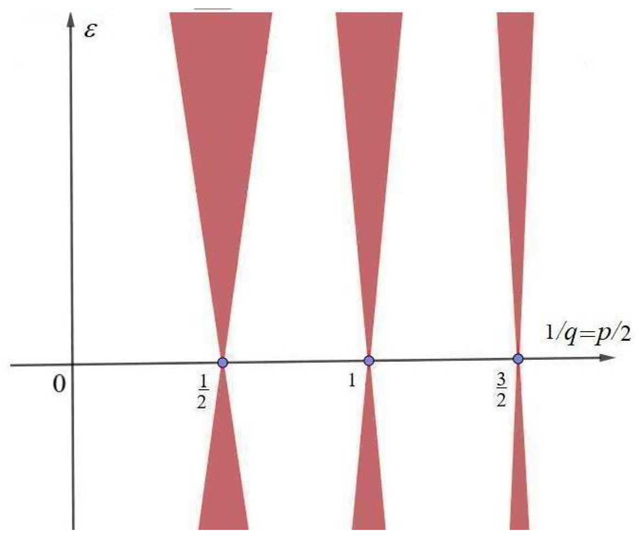
2.1. Parametric Resonance

Mathieu’s equation of a function of time denoted $\mathbf{z}\left(t\right)$, can be written

$$\ddot{\mathbf{z}}+(1+\epsilon cos(q{\omega }_{0}t\left)\right){\omega }_0^2\mathbf{z}=\mathbf{0},$$

(2)

where ${\omega }_0\in {\mathbb{R}}^{+☆}$ is an angular eigenfrequency, $\epsilon \in {\mathbb{R}}^{☆}$ is a very small parameter ($\left|\epsilon \right|\ll 1$) and $q\in {\mathbb{N}}^{+☆}$. The principal period of (2) is ${\displaystyle T_0=2\pi /{\omega }_0}$. The associated system of Hamilton’s equations can be related to a point of the plane constituted by couples $\left(1/q,\epsilon \right)$. All points of the abscissa axis are stable, except points ${\displaystyle q=2/p}$, where $p\in \mathbb{N}$, which are unstable. The amplitude of oscillations of $\mathbf{z}\left(t\right)$ exponentially grows when ${\displaystyle q=2/p}$, where p belongs to $\{1,2\}$.

Figure 2 represents the instability domains associated with Mathieu’s equation. In the plane constituted by couples $\left(p/2,\epsilon \right)$, the instability domains represented in red color touch the abscissa axis at points

$$\left\{{\displaystyle 1/q=p/2,p\in {\mathbb{N}}^{+☆}}\right\}.$$

The abscissas corresponding to the values of $p/2$ on the abscissa axis are the points of parametric resonance; at these points the solutions of (2) become unstable. The instability becomes stronger when the value of $\epsilon$ is increasing [18].

For a given $\epsilon$, the strongest instability of the parametric resonance and subsequent oscillations are observed for $p=1$ (see Figure 2). The correspondence between $\epsilon$ and q comes from the graphs and calculations given in [16,30].

2.2. Plant Experiments on the Earth

The reference angular frequency is ${\omega }_{L_{E_0}}=2\pi \times 1.12\times {10}^{-5}{\mathrm{rad}.\mathrm{s}}^{-1}$, which is associated with the period ${\displaystyle T_{L_E}=24.8}$ h and the small parameter ${\displaystyle {\epsilon }_{{}_{E_0}}=0.47\times {10}^{-8}}$ [30].

Let us consider the $\eta$-disturbance corresponding to variations of the revolution frequency of the Moon around the Earth; then, $\eta$ verifies a differential equation of form (2) and yields instabilities associated with the Rayleigh-Taylor model. The pressure discontinuity $\left[p\right]$ and disturbance $\eta$ across the sap/air-vapor interface vary with ${\epsilon }_{{}_{E_0}}$; and we get

$$\ddot{\mathbf{y}}+(1+{\epsilon }_{{}_{E_0}}\cos ({\omega }_{L_{E_0}}(t-t_0)\left)\right){\omega }_{L_{{}_{E0}}}^2\mathbf{y}=\mathbf{0},$$

We are in case $p=2$ of Mathieu’s equation (see Figure 2), corresponding to small impulsions and instabilities [18]. Note that for ocean tides, the semi-diurnal period of 12.42 h corresponds to a resonance amplitude at least 10 times that of the period of 24.8 h. This does not seem to concern the movements of plant leaves.

2.3. Plant Experiments Inside the ISS

Herein is the crux of our study. The orbital station orbits with a period much shorter than the one of the Moon around the Earth. The reference angular frequency is ${\omega }_{I_{E_0}}=2\pi \times 1.79\times {10}^{-4}{\mathrm{rad}.\mathrm{s}}^{-1}$, which is associated with the period $T_{I_E}=90\min$ and small parameter ${\epsilon }_{I_0}=1.34\times {10}^{-7}$ [16].

Let us consider the $\eta$-disturbance corresponding to variations of the revolution frequency of the ISS around the Earth; then, $\eta$ verifies a differential equation of form (2) and yields instabilities associated with the Rayleigh-Taylor model. The pressure discontinuity $\left[p\right]$ and disturbance $\eta$ across the sap/air-vapor interface vary with ${\epsilon }_{I_0}$; we get

$$\ddot{\mathbf{y}}+(1+{\epsilon }_{I_0}\cos (2{\omega }_{I_{E_0}}(t-t_1)\left)\right){\omega }_{I_{E_0}}^2\mathbf{y}=\mathbf{0},$$

We are in the case $p=1$ of Mathieu’s equation (see Figure 2), corresponding to the optimal parametric resonance coefficient [18]. Coefficient ${\epsilon }_{I_0}$ is 35 times larger than the one associated to the gravitational variations due to the Moon on the Earth; it also corresponds to the case $p=1$ which is the most favorable case for the creation of a parametric resonance.

As predicted by the parametric resonance model, let us note that leaf oscillation cases correspond to the first three multiples of the half-period of rotation of the ISS around the Earth (see Figure 2). Nevertheless, the most efficient case corresponds to a period of 45 min compared to oscillation periods of 90 and 135 min.

Then, as a result inside the ISS, impulses of crude sap give rise to leaf movements of Arabidopsis thaliana, stem and root elongations, and contribute to plant growth. The sap pulses also depend on the distance between the Moon and the Earth and thus on positions of the Moon on its orbit around the Earth.

2.4. Remarks and Conclusions

The purpose of this communication is not to perform experiments but to propose an analytical fluid mechanics model to hopefully interpret the results of some observations made on the ISS. Indeed, the Rayleigh-Taylor model applied in the case of liquid/air-vapor interfaces leads to equilibrium equations, which can undergo instabilities due to parametric resonances. We derive from a mathematical model, a simple similarity with instabilities of fluids in microchannels due to the variations of pressure and velocity for the fluids. As mentioned above, other phenomena must be considered for effects on living organisms. These physical and biological phenomena have been the subject of many other studies and observations which highlight the importance of the Earth’s satellite [2,3,4].

We have only considered the instabilities due to lunisolar tides. We have not examined the dynamics of flows induced by these instabilities. This complementary subject could be the object of additional and voluminous numerical calculations [31]. Plants may have high evaporation in the leaves. This effect would imply a significant circulation of sap, which can be improved by the parametric resonance and which depends on the importance of the sap velocity.

References

1. Moran, N. Osmoregulation of leaf motor cells. FEBS Lett. 2007, 581, 2337–2347. [Google Scholar] [CrossRef] [Green Version]
2. Miles, L.E.M.; Raynal, D.M.; Wilson, M.A. Blind man living in normal society has circadian rhythms of 24.9 h. Science 1977, 198, 421–423. [Google Scholar] [CrossRef] [PubMed]
3. Gluckman, B.J.; Netoff, T.I.; Neel, E.J.; Ditto, W.L.; Spano, M.L.; Schiff, S.J. Stochastic resonance in neuronal network from mammalian brain. Phys. Rev. Lett. 1996, 77, 4098–4101. [Google Scholar] [CrossRef]
4. Bevington, M. Lunar biological effects and the magnetosphere. Pathophysiology 2015, 22, 211–222. [Google Scholar] [CrossRef]
5. Bünning, E. The Physiological Clock. In Circadian Rhythms and Biological Chronometry, 3rd ed.; English Universities Press: London, UK, 1973. [Google Scholar]
6. Klein, G. Farewell to the Internal Clock. In A Contribution in the Field of Chronobiology; Springer: New York, NY, USA, 2007. [Google Scholar]
7. Fisahn, J.; Yazdanbakhsh, N.; Klingelé, E.; Barlow, P.W. Arabidopsis root growth kinetics and lunisolar tidal acceleration. New Phytol. 2012, 195, 346–355. [Google Scholar] [CrossRef] [PubMed]
8. Konopliv, A.S.; Binder, A.B.; Hood, L.L.; Kucinskas, A.B.; Sjogren, L.; Williams, J.G. Improved gravity field of the moon from lunar prospector. Science 1998, 281, 1476–1480. [Google Scholar] [CrossRef] [PubMed] [Green Version]
9. Sorbetti-Guerri, F.; Michel, D. Tree stem diameters fluctuate with tide. Nature 1998, 392, 665–666. [Google Scholar]
10. James, A.B.; Monreal, J.A.; Nimmo, G.A.; Kelly, C.L.; Herzyk, P.; Jenkins, G.I.; Nimmo, H.G. The circadian clock in arabidopsis roots is a simplified slave version of the clock in shoots. Science 2008, 322, 1832–1835. [Google Scholar] [CrossRef] [Green Version]
11. Zajaczhowska, U.; Barlow, P.W. The effect of lunisolar tidal acceleration upon stem elongation growth, nutations and leaf movements in peppermint (Menta × piperita L.). Plant Biol. 2017, 19, 630–642. [Google Scholar] [CrossRef] [PubMed]
12. Crossley, D.; Hinderer, J.; Boy, J.P. Time variations of the European gravity field from superconducting gravimeters. Geophys. J. Int. 2005, 161, 257–264. [Google Scholar] [CrossRef] [Green Version]
13. Barlow, P.W.; Fisahn, J. Lunisolar tidal force and the growth of plant roots, and some other of its effects on plant movements. Ann. Bot. 2012, 110, 301–318. [Google Scholar] [CrossRef] [PubMed] [Green Version]
14. Fisahn, J. Control of plant leaf movements by the lunisolar tidal force. Ann. Bot. 2018, 121, e1–e6. [Google Scholar] [CrossRef]
15. Fisahn, J.; Barlow, P.; Dorda, G. A proposal to explain how the circatidal rhythm of the Arabidopsis thalania root elongation rate could be mediated by the lunisolar gravitational force: A quantum physical approach. Ann. Bot. 2018, 122, 725–733. [Google Scholar]
16. Fisahn, J.; Klingelé, E.; Barlow, P.W. Lunar gravity affects leaf movements of Arabidopsis thalania in the International Space Station. Planta 2015, 241, 1509–1518. [Google Scholar] [CrossRef] [PubMed]
17. Brinckmann, E. ESA hardware for plant research on the International Space Station. Adv. Space Res. 2005, 36, 1162–1166. [Google Scholar] [CrossRef]
18. Gouin, H. Introduction to Mathematical Methods of Analytical Mechanics; Elsevier & ISTE Editions: London, UK, 2020. [Google Scholar]
19. Arnold, V.I. Ordinary Differential Equations; Springer: Berlin, Germany, 1992. [Google Scholar]
20. de Gennes, P.G.; Brochard-Wyart, F.; Quéré, D. Capillarity and Wetting Phenomena: Drops, Bubbles, Pearls, Waves; Springer: New York, NY, USA, 2004. [Google Scholar]
21. Mattia, D.; Gogotsi, Y. Review: Static and dynamic behavior of liquids inside carbon nanotube. Microfluid-Nanofluid 2008, 5, 289–305. [Google Scholar] [CrossRef]
22. Taylor, G.I. The instability of liquid surfaces when accelerated in a direction perpendicular to their planes. Proc. R. Soc. Lond. 1950, A201, 192–196. [Google Scholar]
23. Mellor, G.L. Introduction to Physical Oceanography; Springer: Berlin, Germany, 1996. [Google Scholar]
24. Tavenner, E. The Roman Farmer and the Moon, Transactions and Proceedings of the American Philological Association; The Johns Hopkins University Press: Baltimore, MD, USA, 1918; Volume 49, pp. 67–82. [Google Scholar]
25. Gouin, H. The watering of tall trees—Embolization and recovery. J. Theor. Biol. 2015, 369, 42–50. [Google Scholar] [CrossRef] [Green Version]
26. Brouwer, D.; Clemence, G.M. Methods of Celestial Mechanics; Academic Press: New York, NY, USA, 1961. [Google Scholar]
27. Olson, D.H.; Jacobs, J.W. Experimental study of Rayleigh-Taylor instability with a complex initial perturbation. Phys. Fluids 2009, 21, 034103. [Google Scholar] [CrossRef]
28. Mishra, A.A.; Hasan, N.; Sanghi, S.; Kumar, R. Two-dimensional buoyancy driven thermal mixing in a horizontally partitioned adiabatic enclosure. Phys. Fluids 2008, 20, 063601. [Google Scholar] [CrossRef] [Green Version]
29. Gouin, H. Influence of lunisolar tides on plants. Parametric resonance induced by periodic variations of gravity. Phys. Fluids 2020, 32, 101907. [Google Scholar] [CrossRef]
30. Longman, I.M. Formulas for computing the tidal accelerations due to the Moon and the Sun. J. Geophys. 1959, 64, 2351–2355. [Google Scholar] [CrossRef]
31. Boffetta, G.; Mazzino, A. Incompressible Rayleigh–Taylor turbulence. Annu. Rev. Fluid Mech. 2017, 49, 119. [Google Scholar] [CrossRef] [Green Version]
Figure 1. This shematic is not true to scale. The revolution of the Earth takes place around the pole axis k 0 . The orbit of the ISS is indicated in complete dotted line.
Forests 12 01443 g001
Figure 2. Instability red domain in the parametric resonance case (from [18], pp. 195–200, Figure 9.1).
Forests 12 01443 g002
Publisher’s Note: MDPI stays neutral with regard to jurisdictional claims in published maps and institutional affiliations.