Article

Developing Growth Models of Stand Volume for Subtropical Forests in Karst Areas: A Case Study in the Guizhou Plateau

1
MNR Key Laboratory for Geo-Environmental Monitoring of Great Bay Area & Guangdong Key Laboratory of Urban Informatics & Shenzhen Key Laboratory of Spatial Smart Sensing and Services, Shenzhen University, Shenzhen 518060, China
2
Key Laboratory of Land Surface Pattern and Simulation, Institute of Geographic Sciences and Natural Resources Research, Chinese Academy of Sciences, Beijing 100101, China
3
School of Politics and Public Administration, Hainan University, Haikou 570228, China
4
School of Architecture and Urban Planning, Shenzhen University, Shenzhen 518060, China
*
Authors to whom correspondence should be addressed.
Forests 2021, 12(1), 83; https://doi.org/10.3390/f12010083
Submission received: 16 November 2020 / Revised: 23 December 2020 / Accepted: 11 January 2021 / Published: 14 January 2021
(This article belongs to the Section Forest Inventory, Modeling and Remote Sensing)

Abstract

:
Forest stand volume is one of the key forest structural attributes in estimating and forecasting ecosystem productivity and carbon stock. However, studies on growth modeling and environmental influences on stand volume are still rare to date, especially in subtropical forests in karst areas, which are characterized by a complex species composition and are important in the global carbon budget. In this paper, we developed growth models of stand volume for all the dominant tree species (groups) (DTSG) in a subtropical karst area, the Guizhou Plateau based on an investigation of the effects of various environmental factors on stand volume. The Richards growth function, space-for-time substitution and zonal-hierarchical modeling method were applied in the model fitting, and multiple indices were used in the model evaluation. The results showed that the climatic factors of annual temperature and precipitation, as well as the site factors of stand origin, elevation, slope gradient, topsoil thickness, site quality degree, rocky desertification type and rocky desertification degree, have significant influences on stand volume, and the topsoil thickness and site quality degree have the strongest positive effect. A total of 959 growth equations of stand volume were fitted with a five-level stand classifier (DTSG–climatic zone–site quality degree–stand origin–rocky desertification type). All the growth equations were qualified, because all passed the TRE test (≤30%), and the majority of the R2 ≥ 0.50, above 70% of the RMSE were between 5.0 and 20.0, and above 80% of the P ≥ 75%. These findings provide updated knowledge about the environmental effect on the stand volume growth of subtropical forests in karst areas, and the developed stand volume growth models are convenient for forest management and planning, further contributing to the study of forest carbon storage assessments and global carbon cycling.

1. Introduction

Forest stand volume is one of the key forest structural attributes in estimating and forecasting timber production, fuel accumulation, ecosystem productivity and carbon stock [1,2,3]. Simulating stand volume growth can effectively project forest resource development and thus support sustainable forest management and planning practices [4], especially in mitigating greenhouse effects under the conditions of climate change [5,6]. Most studies focus on the allometric relationship between stand volume and related forest structural variables, such as tree height, basal area, diameter at breast height (DBH), stand density, canopy area, etc. [2,3,7,8], instead of on the growth models for stand volume. Although such allometric equations could estimate the stand volume conveniently, they only provide an assessment for the present but not for the future, showing a weakness in representing the growth of stand volume over time, and thus could not fulfill the need for forest planning. To date, growth modeling for stand volume is still a very important issue in forest mensuration and management [9,10], which urges us to pay full attention to it.
Karst landform, underlain by carbonate rocks (e.g., limestone or dolomite), is widespread globally and accounts for approximately 10–15% of land in the world [11]. The karst landscape of southwestern China, occupies approximately 3.44 million km2 or approximately 36% of the total land area of China and 15.6% of the karst area in the world [12,13]. It is one of the most typical, continuous, and largest karst landscapes in the world [13,14] and is characterized by its strong irregular geomorphology, high erodibility of the limestone substrate and leanness of the soil. Moreover, this karst region is located in the subtropical monsoon humid region with abundant rainfall, mild temperatures and a long growing season, leading to the coexistence of lush vegetation, high biodiversity and high ecosystem fragility [15,16,17]. Vegetation in the region has a unique adaption for drought, rocky establishment and excessive calcium [18], and the representative forest types include mixed mountainous evergreen coniferous forest, evergreen and deciduous broad-leaved forest [15,19]. However, the karst area has experienced a long history of deforestation and reclamation. The two latest large-scale deforestations occurred in the 1950s during the Great Leap Forward and in the 1980s driven by the rapid increase in population and urgent need for food and economic development, causing the forest cover to drop from 45% in the 1950s to 12.6% in the 1980s [20]. The vegetation–soil–landscape relationship deteriorated, resulting in forest degradation to shrubs or grasses and even to rocky desertified land in some areas [18,21]. It was not until 2000, after a series of ecological restoration programs, e.g., the Grain for Green Program, were implemented in the area, that the situation got under control [22,23]. To date, the growth mechanisms of subtropical forests in karst areas, characterized by diverse habitat heterogeneity and complex species composition [15,17,24], have seldom been studied in comparison with other forest ecosystems [13,25]. Studying stand volume growth in karst areas is necessary for understanding the growth mechanisms of this unique forest ecosystem as well as for supporting decision-making for local forest management and planning. Moreover, since forest ecosystem carbon storage in subtropical karst regions is very important to the global C budget due to its special geological conditions and large carbon sequestration potential [26], the growth modeling of forest stand volume—the foundation of biomass and carbon stock estimation—in this area is valuable to mitigate global climate change.
In forest growth modeling, the effect of environmental factors on forest growth, such as climate, site quality, topography, and human disturbance, should not be neglected [27,28,29,30]. Lindner et al. [27] compiled and summarized the existing knowledge about climate change impacts on European forest ecosystems and highlighted that warmer temperatures are expected to result in positive effects on forest growth and wood production, while increasing drought and disturbance risks will cause adverse effects. The study of Luo and Zhang [31] in Yunnan Province, China, found that the growth of stand mean DBH of Pinus yunnanensis was significantly positively correlated with stand age, slope, site index, mean annual temperature and precipitation but significantly negatively correlated with elevation and canopy density. In addition, management practices that influence forest growth, including improved seeds, draining, weeding, fertilization, structure and density shaping, as well as the cessation of deleterious practices—grazing, litter raking, and charcoal burning—would undoubtedly increase forest growth rates greatly in subsequent rotations [32,33,34]. Therefore, the growth curve of the same tree species might vary significantly with changes in climate, topography, management measures or any other environmental factors, and the consideration of environmental factors in stand volume growth modeling can help to improve the accuracy and effectiveness of stand volume forecasting at the regional scale.
Previous studies have developed many forest growth models based on different methods. For example, Piao et al. [28] developed nonlinear regression equations involving stand age, site index and density for estimating stand DBH growth in Korea. Monserud et al. [35] used thin plate smoothing splines to create a spatial model of site indices for lodgepole pine (Pinus contorta) in Canada with inputs of latitude, longitude, elevation, and site index. Yu et al. [36] built a generalized additive model considering climate variables, stand variables and competition variables to simulate the growth of individual tree DBHs in northeastern China. Multiple linear models have been used to develop forest growth models with various environmental variables in eastern Germany [37], Canada [38], China [39], Portugal [40], etc. However, compared with stand volume, more studies focus on DBH, tree height or site index. In addition, regression analysis can only describe certain parts of a complex relationship between environmental and response variables [37], constraining their extrapolation or upscaling to larger areas [41,42]. Moreover, some variables, such as climate factors, only vary slightly in a similar climate zone at the regional scale; thus, their forest growth models are supposed to remain the same, and it is not necessary to put these variables into the fitting equations. At the regional scale, the use of zonal or hierarchical models may be a meaningful tool to describe the important influences of environmental factors in more detail and to improve model precision [37,43]. In the field of forestry, researchers are often confronted with various measurement data that can be ordered into various hierarchical levels—from the individual tree samples in lower levels grouped into an upper hierarchy at the stand level [43]; thus, it is very convenient and common to use these data for zonal or hierarchical modeling. For example, Gara et al. [3] explored the relationship between canopy area and wood volume at four levels: species-specific by site, species-specific across sites, stand level by site, and stand level across sites. Nothdurft et al. [43] used a nonlinear hierarchical mixed model to describe tree height growth of Norway spruce from longitudinal measurements, such as elevation and diameter growth rates. Such principles are also reflected in the fitting of multigrowth curves of the site index for the same tree species [44,45,46,47].
In this paper, taking the Guizhou Plateau as our case study area, we developed stand volume growth models for all dominant tree species (groups), after investigating the effects of various environmental factors, including climate and site conditions, on stand volume, with the usage of a forest inventory spatial dataset of Guizhou province. The Richards growth function, space-for-time substitution and zonal-hierarchical modeling were applied in the model fitting, and multiple indices were used in the model evaluation. Our study attempts to address the following questions: (i) what the current situation of the forest in Guizhou Plateau is; (ii) what the effects of different environmental factors on the stand volume are, with respect to different tree species in the karst area, and which environmental factors have the most significant influence on stand volume; and (iii) building up stand volume growth models for all the tree species with consideration of the environmental effect, and further uncover the stand volume growth pattern in the subtropical karst area.

2. Materials and Methods

2.1. Study Area

The Guizhou Plateau (24°37′~29°13′ N, 103°36′~109°35′ E), covering all of Guizhou Province in southwest China, is located in the east slope zone of the Yunnan-Guizhou Plateau and the upper reaches of the Yangtze River and Pearl River. The 176,167 km2 region mainly inclines from west to east, with complex geomorphology consisting of four basic types: plateaus, mountains, hills and basins. Approximately 92.5% of the land is covered by mountains and hills, and the elevation therein varies significantly from 147.8 m to 2900.6 m (averaging 1100 m) (Figure 1). Called a Karst Province, the Guizhou Plateau is largely underlain by carbonate rocks and occupied by karst landscapes (Figure S1). The karst area covers more than 130,000 km2, representing 73.6% of the plateau and 6.5% of the total karst area of China [21].
Within the East Asian Monsoon climate zone, which has benefitted from uplift of the Tibetan Plateau [48], the Guizhou Plateau has cool humid summers and relatively mild winters. The annual average temperature was 15 °C from 1990 to 2016, and was lowest in January, ranging from 3 to 6 °C, and highest in July, ranging from 22 to 25 °C. The rainfall is abundant with a clear rainy season, and the annual average precipitation reached 1177 mm from 1990 to 2016, with the perennial relative humidity reaching above 70%. Under the influence of atmospheric circulation and topography, the Guizhou Plateau presents apparent regional climatic zonal characteristics, and temperature and precipitation are generally higher in the south and east and lower in the north and west (Figure S2).
The vegetation type in the Guizhou Plateau varies from evergreen coniferous forests to broad-leaved evergreen and deciduous forests with increasing latitude and elevation [49], in which a rich diversity of woody species is harbored [15,17]. However, the long-term and large-scale deforestation and reclamation in the last century have made most of this fragile karst region suffer rocky desertification [50,51]. Much of the forest vegetation had degraded to shrubs, grass and even stony deserts, and many late seral forests were gradually replaced by secondary forests and single-species plantations.

2.2. Data Collection and Treatment

2.2.1. Forest Inventory Spatial Dataset

The forest inventory spatial dataset came from the fourth forest resource planning and design survey (FRPDS) of Guizhou Province. The FRPDS is designed for meeting forest management needs. It investigates the tree species, quantity, quality, structure, function, benefit and distribution of all forests at the county-level scale [52]. The fourth FRPDS of Guizhou province (FRPDSGP) was initiated by the Guizhou Forestry Bureau and conducted by skilled workers of local county forestry departments during 2015–2016 (mostly in 2016). Many stand attributes and site conditions for more than 3 million stands were measured on the ground, including the dominant tree species (group) of a stand, stand age (a), stand volume per hectare (m3 ha−1), average tree height (m), average DBH (cm), stand area, stand origin, elevation, slope gradient, topsoil thickness, site quality degree, rocky desertification type, etc. The FRPDSGP was archived in ArcGIS Geodatabase.gdb format, mapping at a 1:10,000 scale using the Xi’an 1980 coordinate system. Each stand was documented as a record (i.e., a polygon), and each stand attribute or site condition was set as a field. The stand polygons were first drawn from a base map composed of the last phase of FRPDSGP, multi-source satellite images including Landsat TM/ETM+ and HJ-1 A/B images in 2015 and 2016, topographic map, and other basic geographic maps such as administrative boundaries, highway, railway, river and lakes, etc., and then were adjusted and corrected by field survey. The area of a stand was no less than 1 ha.
The stand volume was estimated by the point sampling method using automatic level angle gauge. At least two sample points were set deep inside the forest stands. The workers stuck with the sample points and looked at the trunks of the trees around them (at breast height 1.3 m with DBH ≥ 5 cm) through an angle gauge when conducting field measurements, and each point was measured twice from clockwise and counterclockwise direction to check each other. Sample size was determined by each county or forest management unit which was regarded as a survey population. Data for all counties and forest management units were aggregated to generate provincial statistics. The overall sampling precisions of stand volume were ≥ 85% (α = 0.05) to survey populations with total stand volume ≥ 2 million m3 and were ≥ 80% (α = 0.05) to those with total stand volume <2 million m3 [52,53]. Since the total number of tree species had reached over 300, we categorized them into 36 main dominant tree species (groups) (DTSG) according to the classification system of Chinese Vegetation and the Detailed Rules for the Implementation of FRPDSGP [54,55], with consideration of the density, area, biological, and ecological characteristics of all tree species. The numbers of coniferous and broad-leaved DTSG were 16 and 20, respectively (Table S1), and coniferous occupied 59% of the forest area, while broad-leaved occupied 41%. The spatial distribution of DTSG is shown in Figure S3.

2.2.2. Climate Spatial Dataset

The climate data were derived from the daily meteorological observation data provided by government meteorological stations (http://data.cma.cn) around and inside the Guizhou Plateau in 2016. The ANUSPLIN spatial interpolation method, which is based on thin plate smoothing splines theory and takes into account the effect of topographic factors [56,57], was used to generate the spatial dataset of annual temperature and precipitation with a grid size of 100 m × 100 m.

2.3. Methods

The sampling and statistical analysis of environmental effect analysis were carried out on the R version 3.6.1, with usage of R-packages ggplot2 and psych [58], and the growth modeling and validation for stand volume were carried out on the Curve Fitting Toolbox on MATLAB 2018a [59].

2.3.1. Environmental Effect Analysis

Environmental Factor Selection

We considered 11 potential environmental factors, which were grouped into climatic factors and site factors, to analyze the environmental effect on stand volume and further applied them in the zonal-hierarchical stand volume growth models (Table 1).
Annual temperature and precipitation were taken into consideration as climatic factors. Since the spatial dataset of annual temperature and precipitation were raster format while the forest inventory map was feature format, we first converted the climate raster dataset into point shapefiles and then overlaid them with the forest inventory map to derive the annual temperature and precipitation value for each stand. If more than one point in the climate data fell in one polygon in the forest inventory data (i.e., a stand), they would be averaged.
Site factors include stand origin, elevation, slope gradient, aspect, slope position, topsoil thickness, site quality degree, rocky desertification type and rocky desertification degree. From the stand origin it is possible to infer the land use and human disturbance of a stand, as stands in plantations or forest farms are almost always artificially cultivated, while those in the wild often grow naturally, so here we recognized it as a site factor. The site quality degree is a score value that aims to qualify the site quality for forest growth. It was derived from six individual site factors, i.e., topsoil thickness, soil type, slope gradient, aspect, slope position and traffic location, by using the analytic hierarchy process (AHP) method according to China’s National Forestry Administration [60]. This factor seems to duplicate some other factors; however, we considered it here to compare the significance of the effect of the composite factor with the individual factors and thus to decide whether to use the individual factors or the composite factor in the further zonal-hierarchical modeling. The rocky desertification type denotes whether a stand had suffered land degradation, where soil is seriously or thoroughly eroded in the karst area, while the rocky desertification degree describes how serious the karst land has been rocky degraded. The detailed calculation process of the site quality degree and rocky desertification degree is provided in Part II of supplementary materials. The data of all site factors were obtained from the FRPDSGP. Table 1 describes all the necessary information about the 11 site factors.

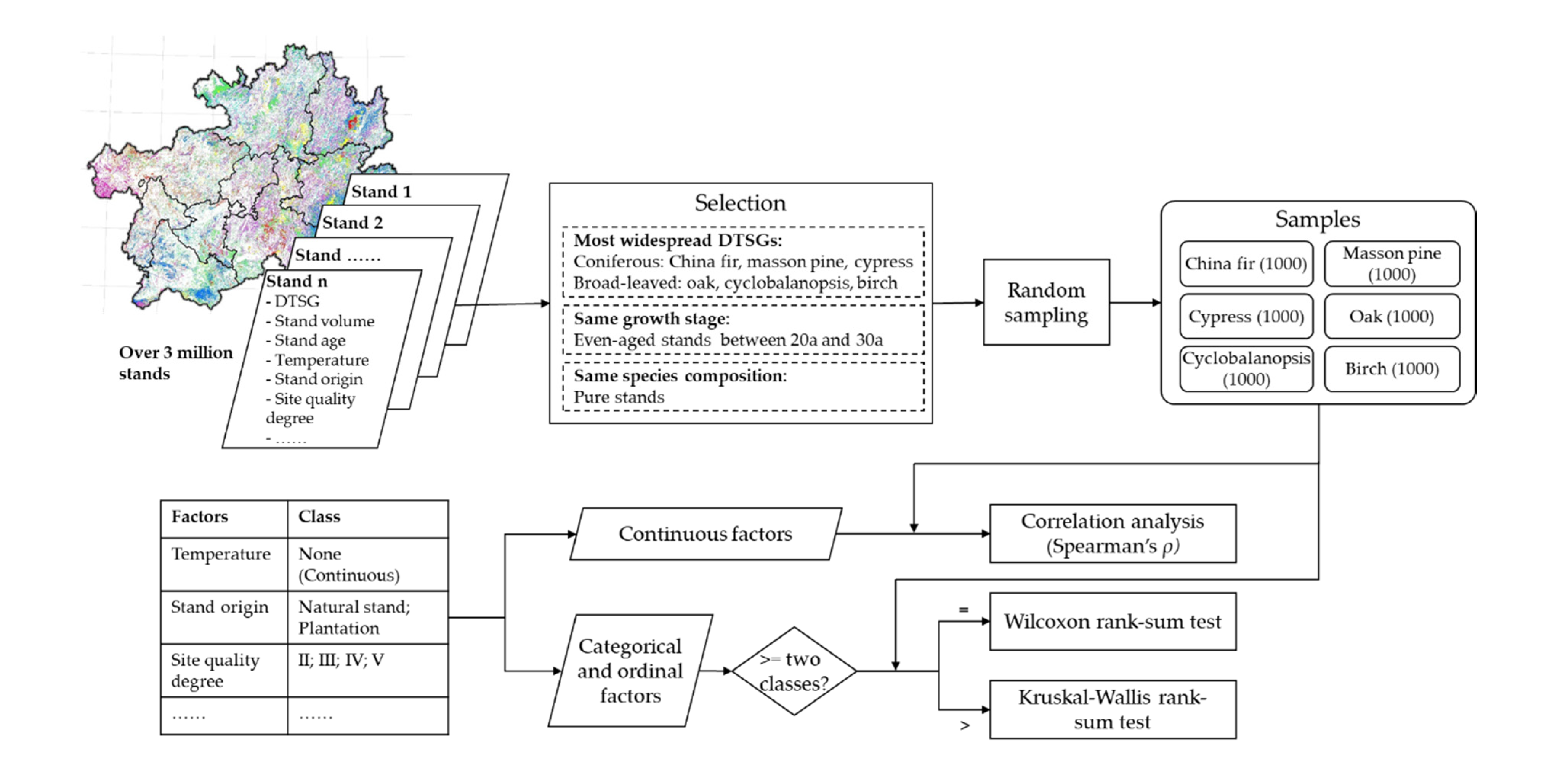
Stand Selection and Sampling for Environmental Effect Analysis

As there were too many forest stands (over 3 million) in the FRPDSGP, stand selection and sampling for environmental effect analysis is necessary. We selected the six most widespread DTSGs with relative single tree species compositions—three coniferous DTSGs, i.e., China fir (Cunninghamia lanceolate (Lamb.) Hook.), masson pine (Pinus massoniana Lamb.) and cypress (Cupressus funebris Endl.), and three broad-leaved DTSGs, i.e., oak (Quercus spp.), cyclobalanopsis (Cyclobalanopsis spp.) and birch (Betula spp.). These six DTSGs occupied approximately 60% of the Guizhou Plateau’s forest area, with China fir and masson pine accounting for approximately 23%, respectively, followed by cypress (4.5%), oak (3.0%), cyclobalanopsis (2.9%) and birch (2.5%). To remove the influence of different growth stage and complicated species composition, we only selected the even-aged pure stands of the six tree species with stand ages between 20 and 30 years as our sample populations. One thousand samples were randomly selected from each of the above six populations.

Statistical Analysis for Revealing the Effect of Environment Factors on Stand Volume

Stand volume here is expressed on a per-hectare-land area basis. As all the stand volumes of the six DTSGs had skewed distributions (Figure S4), to reveal the relationship between the various environmental factors and stand volume in the Guizhou Plateau, correlation analysis (using the Spearman rank correlation coefficient, i.e., Spearman’s ρ) was used for continuous variable (i.e., temperature, precipitation, elevation, slope gradient and topsoil thickness) analysis. Two nonparametric hypothesis test methods—Wilcoxon rank-sum test and Kruskal-Wallis rank-sum test—were employed for categorical and ordinal variable analysis. The Wilcoxon rank-sum test [61], also known as the Mann-Whitney U test, was used to compare the stand volume between two groups divided by the factors with two classes (i.e., stand origin). The Kruskal-Wallis rank-sum test [62] was used to test whether there were significant differences among the stand volumes of more than two groups, which were divided by the factors with more than two classes (i.e., aspect, slope position, site quality degree, rocky desertification type and rocky desertification degree).
A detailed workflow for analyzing the effect of environment factors on stand volume in Guizhou Plateau is displayed in Figure 2.

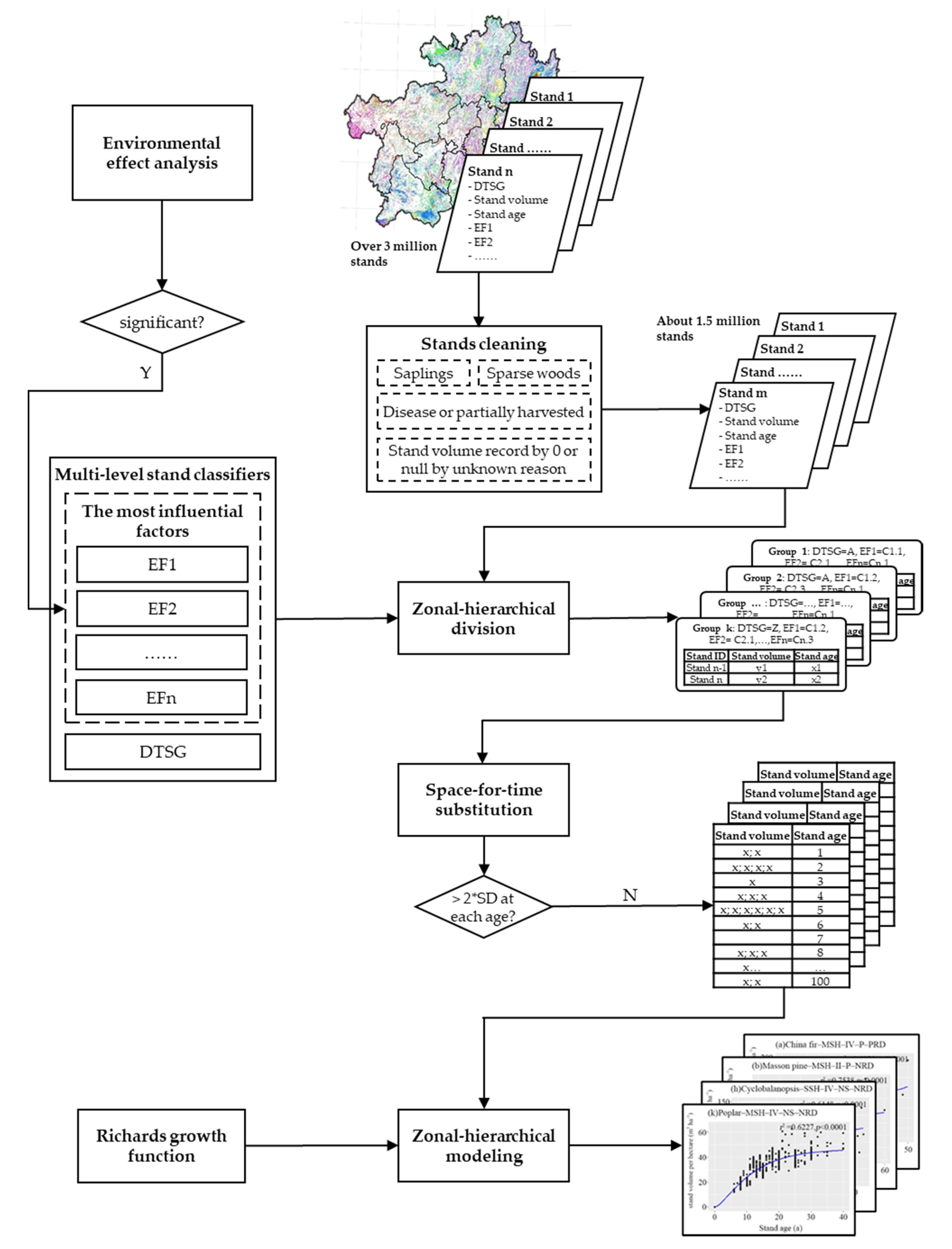
2.3.2. Stand Volume Growth Modeling

Model Fitting

We used the Richards growth function [63] to develop the growth models of stand volume. The Richards growth function, also called the Chapman-Richards function, was based on von Bertalanffy’s growth theory [64] and embodies commonly used growth functions as monomolecular, Gompertz, and logistic equations [63]. This model has been widely applied in forestry owing to its flexibility, accuracy, and meaningful analytical properties [65,66,67], as well as represents the S-shaped curve law of slow-fast-slow characteristics in stand volume growth. The equation is as follows:
V = a ( 1 e b × a g e ) 1 1 c
where V is the stand volume per hectare (m3 ha−1), age is the stand age (a) equal to the average tree age in the stand, and a, b and c are model parameters. With the change in the value of parameter c, the Richards function can be transformed into the logistic equation (c < 0), Mitscherlich equation (c = 1) and Gompertz equation (c→∞), showing good adaptability and high flexibility [68,69]. The values of parameters a, b and c are all greater than 0.
As we had only one phase of forest inventory data, we used space-for-time substitution [70] to obtain stand volumes with time series from different aged stands. The space-for-time substitution, also known as the chronosequence approach, has been an important and effective tool for generating time series from contemporary spatial patterns and studying the temporal dynamics of plant communities [71,72] (Figure 3). However, one challenge of this approach is that it assumes that spatial and temporal variations are equivalent [70], which is impossible for the high heterogeneity of the study area. More importantly, the environmental effect should not be neglected. Therefore, the zonal-hierarchical model method was used to build a set of equations [3,43] (Figure 4). First, we removed all the stands of saplings (with no stand volume recorded) and sparse woods, as well as the stands disturbed by disease or partially harvested recently, and any other stands with stand volume record by 0 or null by unknown reason; after doing this, only approximately 1.5 million stands were left. Second, we divided all 1.5 million stands into groups at several levels, according to the DTSG and major environmental factors, which depend on further environmental effect analysis. Third, we applied the space-for-time substitution to generate stand volume–age series for each stand group, and data greater than twice the standard deviation of stand volume at each stand age were excluded to reduce noises (affected by other less important factors or other ecological processes) and improve the reliability and availability of the models [73]. Finally, we used the Richards growth function to fit the allometric relation between the stand volume and stand age for each stand group. Therefore, Equation (1) can be rewritten as:
V i , e f 1 , e f 2 , , e f n = a i , e f 1 , e f 2 , , e f n ( 1 e b i , e f 1 , e f 2 , , e f n × a g e ) 1 1 c i , e f 1 , e f 2 , , e f n
where i is the DTSG of a stand, ef1, ef2 to efn refers to the values of environmental factors that significantly impact the stand volume, and n ≤ 11.
A workflow for growth model fitting on stand volume with application of zonal-hierarchical modeling and space-for-time substitution in Guizhou Pleteau is showed in Figure 5.

Model Evaluation

Eighty percent of the data in each stand group were randomly chosen for model fitting (i.e., modeling samples), and the remaining 20% were used for model validation (i.e., validation samples). The total relative error (TRE), coefficient of determination R2, root mean square error (RMSE), and prediction accuracy (P) were used to measure the goodness-of-fit of the models [31,73,74]. TRE calculates the absolute difference between the observed and estimated data [75] and was chosen to decide whether the fitting equation passed the test if the TRE was less than 30% [73,76]. P evaluates the forecast accuracy of the model [73]. In addition, residual graphs were used to reveal the homogeneity of variance and outliers of residuals between predicted and observed values [77]. The calculation of the TRE and P are listed below:
T R E = i = 1 n | y i y ^ i | ( 2 i = 1 n y ^ i ) × 100 %
P = ( 1 t α i = 1 n ( y i y ^ i ) 2 y ¯ ^ i n ( n K ) ) × 100 %
where yi is the observed value of modeling samples, y ^ i is the predicted value for modeling samples, n is the size of modeling samples, tα is the value of the t distribution when the significance level α = 0.05, K is the number of model parameters, and y ¯ ^ i is the mean predicted value for modeling samples.
After all the stand volume growth equations were fitted, validation was conducted by comparing the actual observation of validation samples with model prediction. The RMSE were taken as our validation indicators, the smaller RMSE reflect the higher accuracy and applicability of the models.

3. Results

3.1. Statistics of Stand Volume in 2016

In 2016, the total stand volume of all DTSGs in the Guizhou Plateau reached 452.47 million m3, with a total forest area of 7.24 million ha, and the stand volume reached 62.47 m3 ha−1 (Table 2). The living volume of coniferous-dominated forests (322.66 million m3) was 2.5 times that of broadleaved-dominated forests (129.80 million m3), while the former stand volume per hectare (75.52 m3 ha−1) was 0.7 times higher than the latter (43.70 m3 ha−1). Except for mixed forests, the forests dominated by Chinese fir and masson pine had the highest living volume in the study area, reaching 138.32 million m3 (30.57%) and 135.75 million m3 (30.02%), respectively, and both occupied two-thirds of the living forest volume in the Guizhou Plateau, followed by cypress (2.65%), Yunnan pine (2.65%), and cryptomeria (2.64%). The stand volumes of Chinese fir and masson pine reached 81.59 m3 ha−1 and 80.65 m3 ha−1, respectively, which were still the highest among all the DTSGs, followed by maple (75.47 m3 ha−1), ebony (72.72 m3 ha−1), and cryptomeria (70.83 m3 ha−1). From Table 2, we can also clearly draw out that the forests in Guizhou Plateau were still quite young (only approximately 20 a); in other words, most of them were newly planted or naturally germinated; thus, the stand volume of most DTSGs was relatively low, especially Chinese yew and willow. Please note that our statistical results only represented the situation of the DTSG but not all the forests in the Guizhou Plateau. The living volume was mainly concentrated in the southeastern part of the study area (Figure S5)

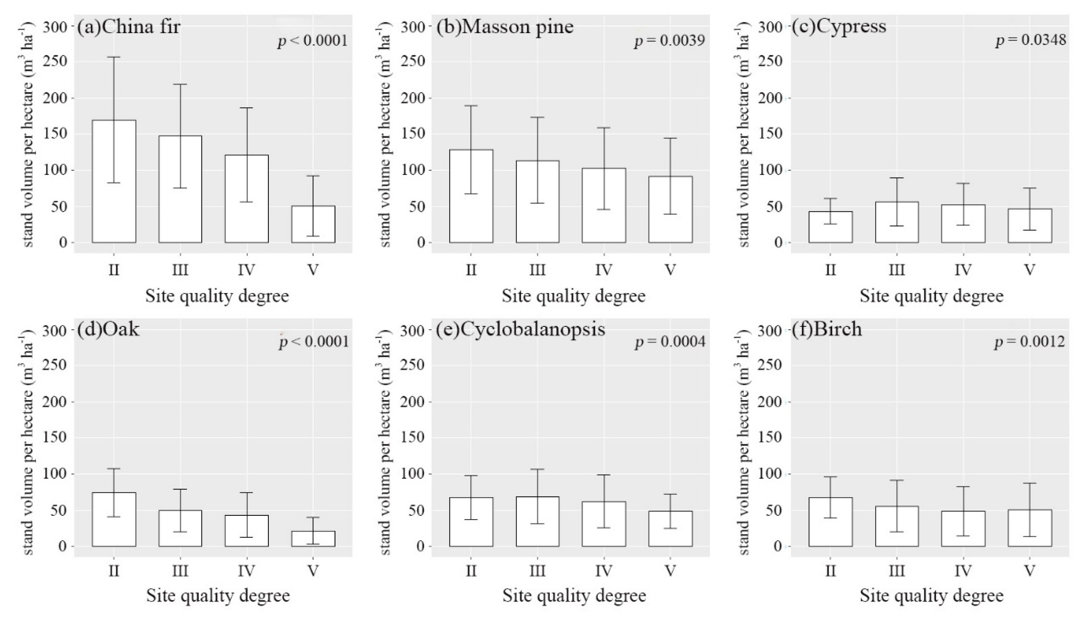
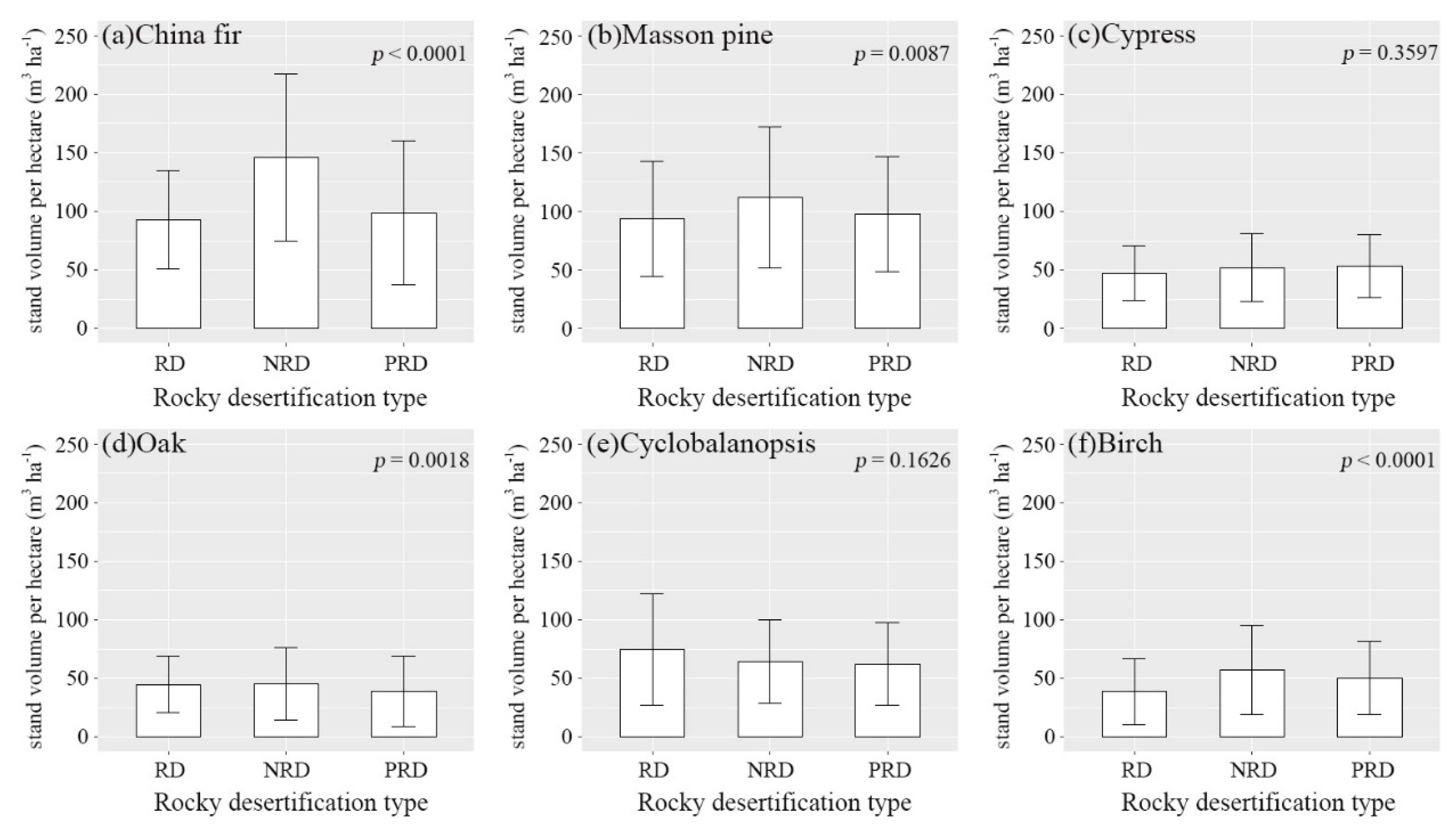
3.2. Environmental Effect on Stand Volume

The correlation analysis, Wilcoxon rank-sum test and Kruskal-Wallis rank-sum test results showed that the climatic factors annual temperature and precipitation, as well as the site factors stand origin, elevation, slope gradient, topsoil thickness, site quality degree, rocky desertification type and rocky desertification degree had a relatively significant influence on the stand volume.
For the continuous variables, including the annual temperature and precipitation in climatic factors and the elevation, slope gradient, and topsoil thickness in site factors, our correlation analysis results showed that all of them had a significant correlation with stand volume of the six selected DTSGs (Table 3, Figures S6–S10). The topsoil thickness had the strongest positive effect on stand volume, as all six DTSGs passed the significance test at the p = 0.01 level, and all slopes and Spearman’s ρ values were greater than 0. The stand volume was also significantly influenced by the climate. Five out of the six DTSG stand volumes were significantly correlated with the annual precipitation, which was positive for China fir (p < 0.01), cypress (p < 0.05), cyclobalanopsis (p < 0.05) and birch (p < 0.01) and negative for oak (p < 0.01). Moreover, four out of the six DTSG stand volumes were significantly correlated with the annual temperature, which was positive for China fir (p < 0.01), cyclobalanopsis (p < 0.01) and birch (p < 0.01), and negative for oak (p < 0.01). For elevation, significant negative correlations were found in most of the tree species, including China fir (p < 0.01), cyclobalanopsis (p < 0.05) and birch (p < 0.01), whereas significant positive correlations were found in oak (p <0.01). All stand volumes of the six DTSGs were negatively and mostly significantly (except cypress) correlated with the slope gradient (p < 0.05). Note that we did not exclude the influence of other factors on stand volume while conducting correlation analysis for one factor due to the complexity of source data; hence, the Spearman’s ρ was inevitably relatively low, but still, the environmental influence was revealed through the significance and slope value.
The results of the Wilcoxon rank-sum test showed that there were significant differences between natural forest and plantation in stand volume of masson pine, cypress, oak and birch (p < 0.01) (Table 4, Figure S11). The stand volumes of plantations dominated by masson pine, oak and birch were 18.48%, 37.51% and 20.81% significantly higher than those of natural forests on average, respectively, whereas the plantation dominated by cypress was 7.16% less than those of natural stands. There was no significant difference between the stand volume of natural forest and plantation of cyclobalanopsis. Moreover, we did not compare the stand volume difference between the two origins of China fir for the very few natural stands in this tree species.
The results of the Kruskal-Wallis rank-sum test revealed that only the site quality degree, rocky desertification type and rocky desertification degree affected the majority of the six DTSGs. All six selected DTSGs were found to have statistically significant differences (p < 0.05) in stand volume between the different site quality degrees, and their stand volume decreased overall with the decline in site quality degree except cypress (Figure 6). There were significant differences (p < 0.01) between the three rocky desertification types in stand volume of four tree species—China fir, masson pine, birch and oak, and their stand volume basically followed the rule of rocky desertified < potential rocky desertified < nonrocky desertified (Figure 7). For rocky desertification degree, since the three broad-leaved tree species were not (or could not be) distributed in severe rocky desertified land, only stand volumes with degrees of slight and moderate desertification were compared (Figure 8). It appeared that there were statistically significant differences in stand volume between different rocky desertification degrees in masson pine (p < 0.05), cypress (p < 0.05) and cyclobalanopsis (p < 0.01), following the order of slight > moderate > severe overall. Only the stand volumes of oak (p < 0.01) and birch (p < 0.05) were significantly different among the multiple aspects, whereas the other four DTSGs were not (Figure S12). The slope position only significantly affected the stand volume of oak (p < 0.01) but not the others (Figure S13).
We ranked the 11 environmental factors according to the significance of their correlation with stand volume of the six DTSGs (Table 5). The results showed that topsoil thickness was the most influential environmental factor on stand volume, and all six DTSGs had a very significant relationship (p < 0.01). The site quality degree was the second most powerful factor to present the environmental effect on stand volume; only cypress passed the significance test at the p = 0.05 level, while the others passed at the p = 0.01 level. The environmental factors ranked from third to sixth were precipitation, slope gradient (tied for third), stand origin, temperature and rocky desertification type (tied for sixth).

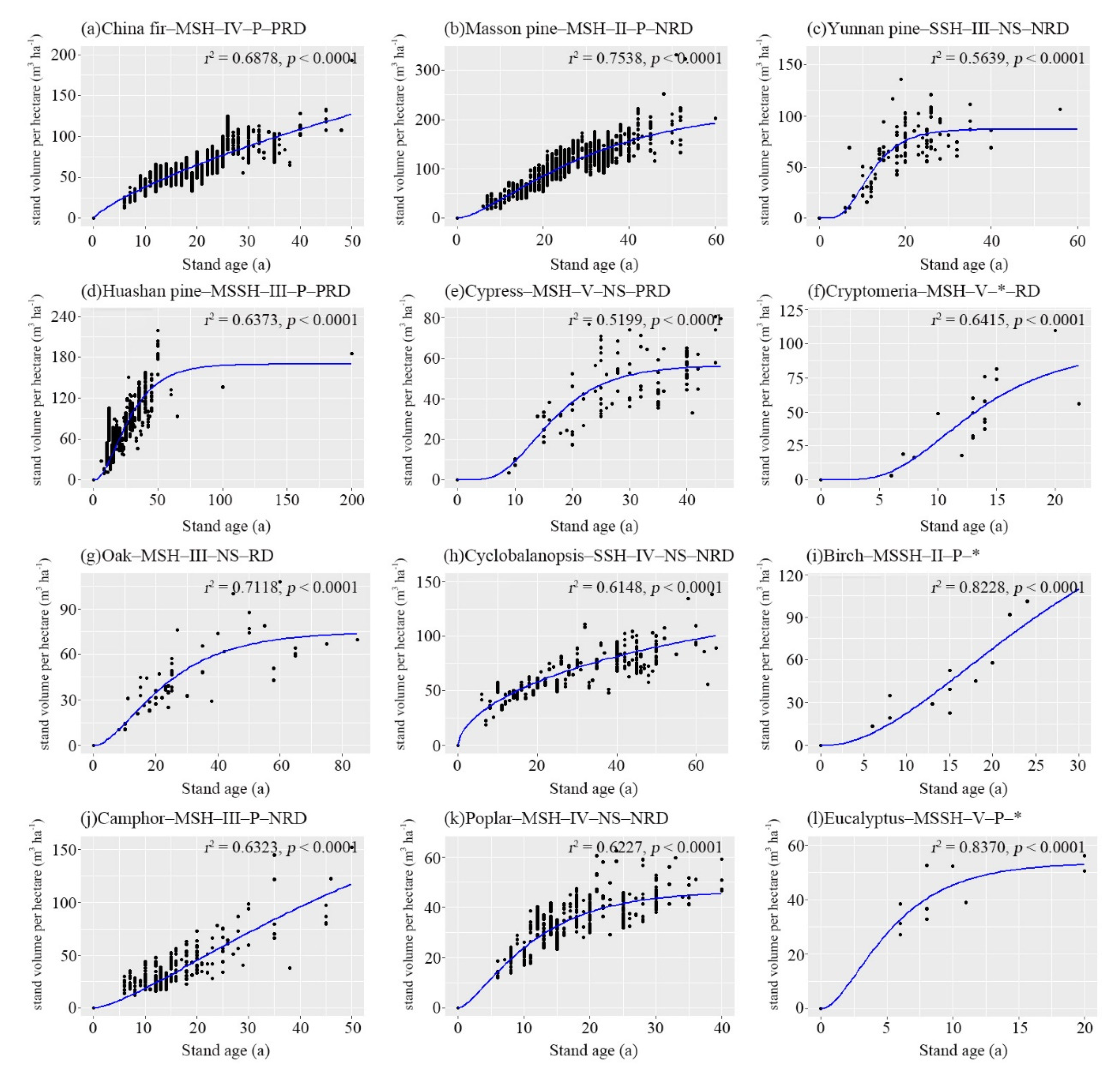
3.3. Growth Modeling of Stand Volume

On the basis of the results above, we chose the most influential environmental factors, i.e., topsoil thickness, site quality degree, precipitation, slope gradient, stand origin, temperature and rocky desertification type, to group the forest stands for zonal-hierarchical modeling. As the topsoil thickness, slope gradient, precipitation and temperature were continuous variables that could not be used for grouping, while the site quality degree is a composite factor involving topsoil thickness and slope gradient, and both the precipitation and temperature represent the climate condition, we further combined the DTSG and the seven environmental factors into a five-level stand classifier, i.e., DTSG–climatic zone–site quality degree–stand origin–rocky desertification type, to divide all the 1.5 million stands in Guizhou Plateau into several groups. The spatial distribution of climate zones was derived from The Ecological Function Regionalization of Guizhou Province approved and implemented by the Guizhou provincial government. We further combined the original five ecological function zones into three climate zones, i.e., mid-subtropical humid (MSH) climate zone, mid-subtropical subhumid (MSSH) climate zone, and south subtropical humid (SSH) climate zone (Figure S14). It should be noted that under the division by the multilevel classifiers, the samples of some stand groups would be too few for model fitting or even missing; at this time, these stand groups will be merged into the upper-level or adjacent groups.

3.3.1. Goodness-of-Fit

A total of 959 growth equations of stand volume were fitted for all the stand groups divided by the five-level stand classifier based on the Richard growth function. As the number was too large, all the parameters and statistics of the growth equations are detailed in Part III of supplementary materials, Table S8. To provide an impression of the goodness-of-fit and typical model trends, several graphs are presented showing stand volume versus stand age (Figure 9). The black dots represent actual observations of modeling samples, while a blue line indicates the predicted curve of the dependent variable. The S-shaped curves clearly illustrated the slow–fast–slow or fast–slow characteristics of stand volume growth, while they varied significantly among the different combinations of DTSG and environmental factors.
All the TREs of the stand volume growth models were less than 30%, suggesting that all the models passed the test and were qualified. The TRE of most stand volume growth equations was within 1% and even equals 0 in 24 stand volume growth equations, e.g., the equations for planted masson pine in MSH–degree V–NRD forestland, and natural Huashan pine in MSSH–degree III–RD forestland.
The majority of the coefficient of determination R2 associated with the built-up growth models reached over 0.50, indicating that at least half of the variance is accounted for by the models. The greatest R2 was found in the volume growth equation for planted willow in MSH–degree III–RD forestland, which is as high as 0.9998. In addition, 33 stand volume growth equations reached over 0.9, e.g., the equations associated with natural masson pine in MSSH–degree III–NRD forestland.
The RMSE values of above 70% of the growth equations were between 5.0–20.0, implying that the predictions from the equations were relatively close to the actual observations. The minimum RMSE of the volume growth equation came from the planted willow in MSH–degree III–RD forestland, reaching only 0.01, followed by the other coniferous DTSG in MSSH–degree II–NRD forestland with RMSE = 0.55. The maximum value of RMSE existed in the volume growth equation of natural beech in MSH–degree III–PRD and RD forestland, reaching 39.97.
The P of more than 80% of the growth equations was above 75%, revealing that our models were able, to a large extent, to forecast accurately for most of the tree species in the study area. The highest P reached 99.94%, which was found for the stand volume growth models for planted willow in MSH–degree III–RD forestland. In addition, there were 427 stand volume growth equations with P > 90%, such as the equations for fir in MSH forestland, planted masson pine in MSH–degree II–NRD forestland, etc.

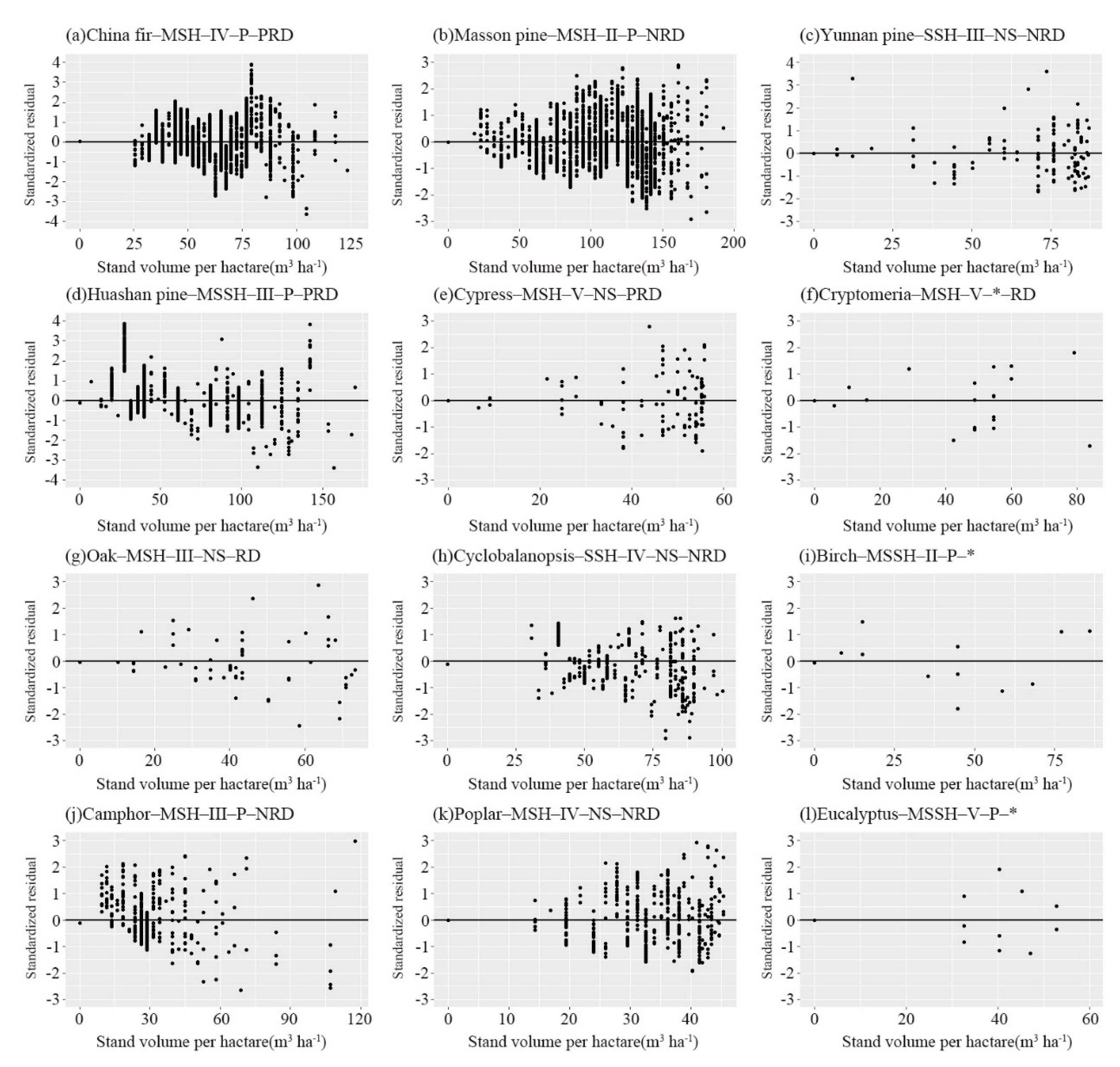
3.3.2. Residual Analysis
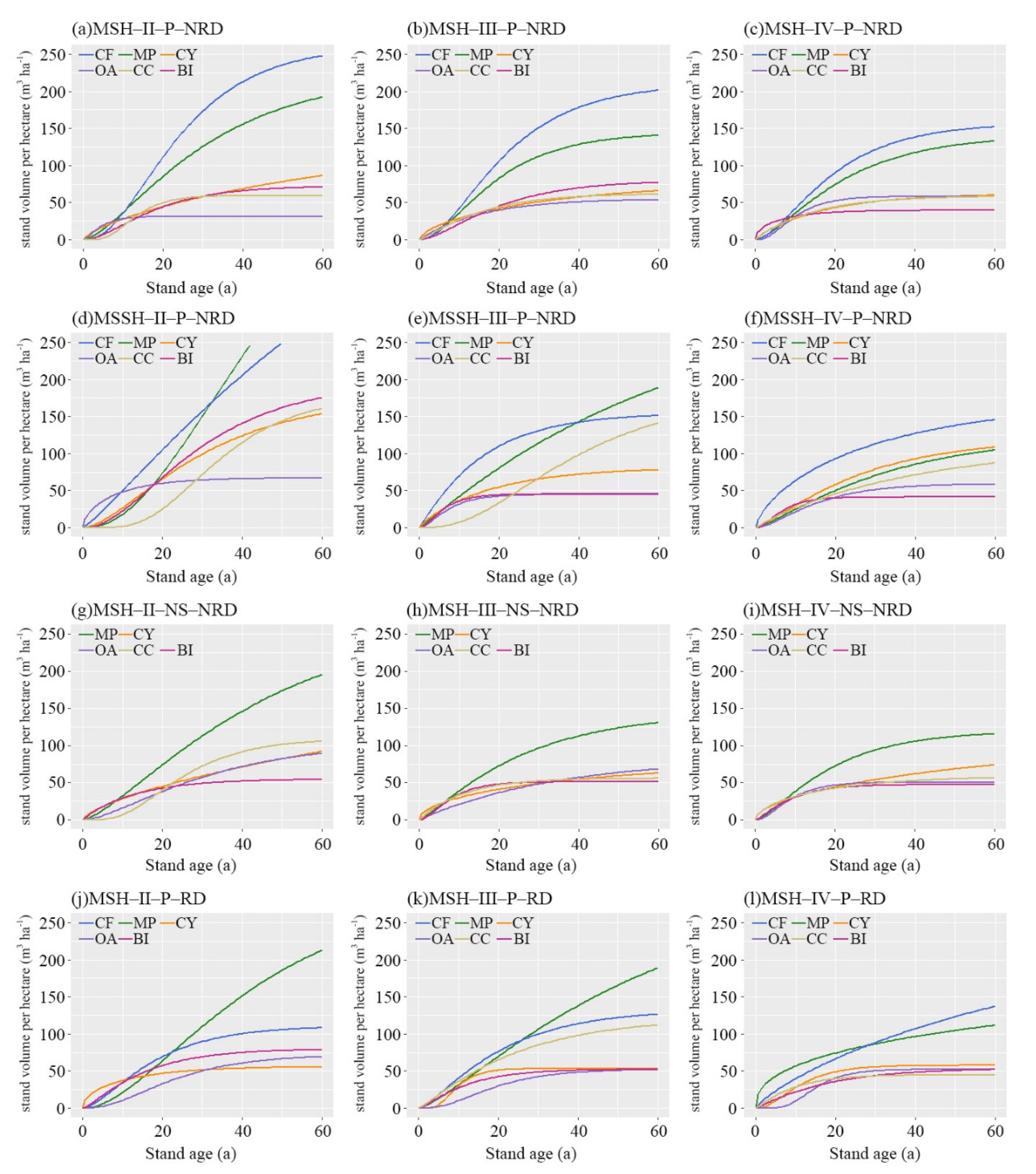
Residual graphs were constructed to illustrate the dispersion of residuals between the actual observations and model predictions (actual minus predicted) versus stand age. The results found that all the residuals were within the range of ±3 times the standard deviation of the mean residual when distributed randomly along with stand age without obvious trends; therefore, all the built-up models could be assumed to be relatively reasonable. Some instances of the residual graphs are shown in Figure 10.

3.3.3. Validation

All the RMSE values between the actual observations of validation samples and the model predictions were lower than 40, and more than 50% were between 5.0 and 20.0. The lowest RMSE value was only 0.01, which was found for the stand volume growth models for planted willow in MSH–degree III–RD forestland, while the greatest RMSE reached 39.71 in association with the stand volume growth models for metasequoia in MSH–degree II forestland.
The validation results reflected the reliability and applicability of the fitted models, indicating that our models would effectively simulate and forecast the growth of stand volume in the Guizhou Plateau in a certain period.

4. Discussion

4.1. Growth of Stand Volume in Guizhou Plateau

Analyzing the growth status of stand volume in the Guizhou Plateau, such as the growth rate, growth upper limit, and the year of growth slowing down, would help to understand the growth patterns of the main tree species in this region, and provide a scientific basis and decision support for forest management and planning to governments in local regions or regions with similar climate and geographical conditions.

4.1.1. Growth Rate

We took the six most representative DTSGs, namely, China fir, masson pine, cypress, oak, cyclobalanopsis and birch as examples, and selected their stand volume growth curves in forestland within MSH and MSSH, which are denoted by degrees II, III and IV, naturally grown and planted, RD and NRD, in order to compare the stand volume growth rate of different DTSGs under various environmental conditions. The results are shown in Figure 11. From each plot in Figure 11, we determined that the stand volume growth rates of coniferous DTSG were basically higher than those of broad-leaved DTSG in the Guizhou Plateau, especially China fir and masson pine. The stand volume of China fir grew fastest in the NRD forestland, followed by masson pine, whereas the highest growth rate was found for masson pine in the RD forestland, followed by China fir. In most cases, the stand volume growth rates of cypress were close to those of broad-leaved DTSG. In the MSH zone, the stand volume growth curves of the three broad-leaved trees were relatively close to each other but differed largely in the MSSH zone. A significant effect of the site quality degree on stand volume growth could be found by comparing each column in Figure 11. With the decline in the site quality degree, the growth rates of stand volume decrease remarkably, especially in coniferous DTSG. By comparing the first and second rows of Figure 11, it was found that climatic zones had a significant influence on the stand volume growth curves: the growth rates of stand volume of all plantations in the degree II forestland within the MSSH zone increased significantly compared with those within the MSH forestland; however, the increment decreased rapidly as the site quality downgraded, especially the masson pine, whose growth rates became even lower than MSH zone in the MSSH–degree III and IV forestland. There were obvious differences between different stand origins in the broad-leaved stand volume growth curves in the MSH–degree II–NRD forestland when comparing the first and third rows in Figure 11, but this situation was not the case for the coniferous and in the other site quality degrees. The comparison between the first and fourth rows of Figure 11 suggests that there were only a few changes between the RD and NRD forestland in the selected stand volume growth rates in the MSH zone, except for China fir, which declined dramatically in the RD area.
To reveal the growth rate rules of all stand volumes in the Guizhou Plateau, we calculated the growth rates every five years of the 959 growth curves until 100 years. The majority of the stand volume growth rates ranged from 0 to 5 m3 ha−1 a−1, accounting for 68.72%. Twenty-six percent of the maximum growth rates of stand volume were distributed between the range of 3–4 m3 ha−1 a−1, followed by 4–5 m3 ha−1 a−1 (18.77%), 2–3 m3 ha−1 a−1 (16.68%), and 6–10 m3 ha−1 a−1 (16.16%). Most of the growth curves (41.19%) peaked in the years between 0 and 5, followed by the years between 5 and 10 (25.65%) and 10 and 15 (18.98%), indicating that the forest stand volume in the Guizhou Plateau grew fast in the sapling and young forest stages. Almost all of the lowest growth rates of the growth curves (88.11%) were concentrated in the last five years before 100, i.e., 95–100, implying that the stand volume growth declined with increasing stand age after their flourishing growth period.

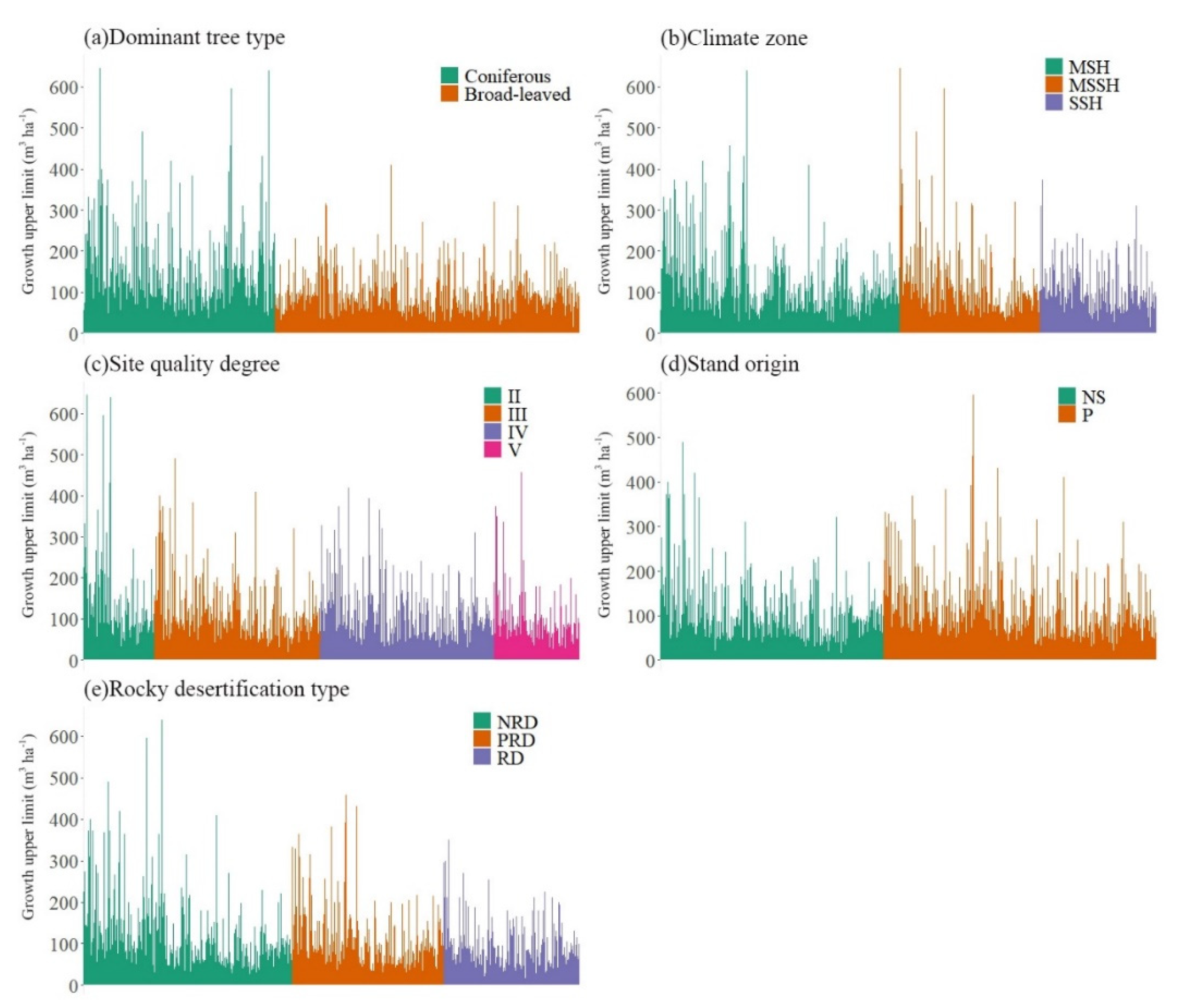
4.1.2. Growth Upper Limit

The parameter a of the Richards growth function represents the theoretical maximum value of stand volume growth. According to the a column in Part III of supplementary materials, Table S8, the growth upper limits of all stand volumes in the Guizhou Plateau were concentrated in the range of 50–100 m3 ha−1, accounting for 44.84%, followed by 50–100 m3 ha−1 (20.13%), 100–150 m3 ha−1 (15.43%), and 150–200 m3 ha−1 (9.18%). The maximum value of stand volume growth upper limit was in reference to masson pine in MSSH–degree II forestland, reaching 644.90 m3 ha−1, while the minimum value corresponded to the plantation of broad-leaved mixed tree species (groups) in SSH–degree II–PRD and RD forestland, only 14.54 m3 ha−1.
Figure 12 demonstrates the distribution of the growth upper limit among different DTSG, climatic zones, site quality degrees, stand origins and rocky desertification types. The growth upper limits of coniferous stand volume were significantly higher than those of broad-leaved stands after the t-test (p < 0.01) (Figure 12a), averaging 137.56 m3 ha−1 and 54.54% higher than the broad-leaved stand volume. The highest growth upper limits corresponded to coniferous trees, such as masson pine, Yunnan pine, and China fir, while the lowest referred to the broad-leaved trees, including locust, camphor, and melia. The growth upper limit of stand volume in the MSH zone reached 110.49 m3 ha−1, approximately 12.83% higher (p < 0.05) than that in the SSH zone (Figure 12b). For the growth upper limit of stand volume at different site quality degrees, except for the nonsignificant difference between degree III and degree IV, the rest all had significant differences: degree II (131.16 m3 ha−1) > degree III (108.23 m3 ha−1) > degree IV (104.39 m3 ha−1) > degree V (90.81 m3 ha−1) (Figure 12c). From the perspective of stand origin, the average upper limits of stand volume of plantations (111.06 m3 ha−1) were higher than those of natural stands (102.77 m3 ha−1), but the differences were not significant (p > 0.05) (Figure 12d). Although there were no significant differences between the NRD and PRD forestlands (p > 0.05) in the upper limits of stand volume, both NRD and PRD forestlands were noticeably higher than RD forestlands (p < 0.05) (Figure 12e), which could be sorted in descending order as follows: NRD (122.22 m3 ha−1) > PRD (111.97 m3 ha−1) > RD (96.94 m3 ha−1). The distribution of the growth upper limits of stand volume basically complied with the plant growth pattern in Guizhou Plateau [15], which indicates that the fitted growth equations are relatively reasonable.

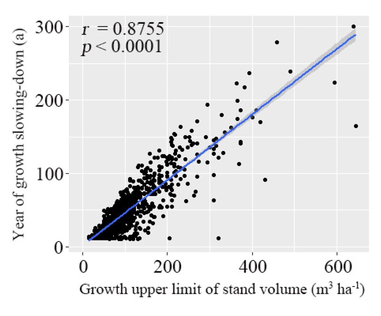
4.1.3. Years of Growth Slowing Down

As the stand volume growth curves presented slow–fast–slow or fast–slow characteristics, we assumed that when the stand volume increment of a certain year was 0.5 m3 ha−1 less than the previous year—based on the built-up growth equations—the growth curves would gradually flattened with the increase of stand age, and the stand volume growth would tend to reach a steady state. Most of the stand volume growth curves in Guizhou Plateau basically slow down within 50 a, accounting for 63.51%, including 36.50% within 30 a and 27.01% within 30–50 a. In addition, 14.81% and 11.47% of the stand volume curves slow down within 50–70 a and 70–100 a, respectively, followed by 100–150 a (7.61%) and above 150 a (2.61%). The years of growth slowing down were significantly and positively correlated with the growth upper limits (r = 0.88, p < 0.01); the higher the growth upper limit was, the greater the number of years of growth slowing down (Figure 13).

4.2. Environmental Effect on Stand Volume in Guizhou Plateau

In this research, we found that both the climatic factors of temperature and precipitation significantly affected the growth of stand volume, but plant responses varied among the species. Previous studies have revealed that regional climate warming extends the growing season and promotes summer photosynthesis, thus stimulating vegetation growth [78,79,80], particularly in regions where water is nonlimiting [81,82]. Nevertheless, other studies have found that if the temperature in the growing season is too high (generally close to or exceeds the ecological optimal temperature for tree growth) without sufficient water supply, the high temperature will inhibit tree growth due to accelerated transpiration [83,84]. For precipitation, increasing precipitation can enhance soil moisture and atmospheric humidity and promote the production of new leaves and branches as well as accelerate biomass accumulation during the growing season, thus facilitating the growth of trees [85,86], especially in arid and semiarid regions due to the lack of rainfall and large evaporation [87,88,89]. However, aerobic respiration of tree roots will be affected if the precipitation is sufficient or too much, e.g., mineral absorption reduction and ethanol accumulation [90,91]; at this time, precipitation is not correlated with radial growth of trees or even negatively correlated, especially in humid regions [92,93]. Furthermore, the biological traits of different tree species, e.g., optimum temperature, moisture and nutrients, vary greatly even in the same area, which might result in different or even opposite relationships between vegetation growth and climate conditions [85]. In this paper, the stand volume of China fir, cyclobalanopsis and birch all presented significant positive correlations with the annual temperature and precipitation, whereas oak, cypress and masson pine did not, implying that while some tree species (groups) in the Guizhou Plateau are still comfortable with the current climate situation, others might be under stress, which should raise our awareness in forest management and planning.
Additionally, site factors, such as topsoil thickness, elevation, slope gradient, stand origin, rocky desertification type and rocky desertification degree, were found to be significantly correlated with stand volume. The karst landscape of the Guizhou Plateau is characterized by extremely slow soil formation from the underlying limestone and very shallow and patchy soils with a low water retention capacity [13,14]. Since topsoil thickness is one of the important indices reflecting the stock of soil orange matter, water and nutrients [94,95], vegetation species and plant growth are largely constrained by topsoil thickness [96], especially in karst areas. Elevation mainly influences vegetation growth indirectly by causing vertical changes in climate conditions. The climate shifts toward more stressful conditions for plant growth with increasing altitude, such as lower temperatures, higher precipitation, longer snow cover, lower atmospheric pressure and higher shortwave radiation [97,98]. The slope gradient is a crucial driver of hillslope soil erosion [99,100], which can impact vegetation growth by influencing the magnitude of surface runoff and soil loss [54,101]. Moreover, the gravity generated by excessive steep slopes is also detrimental to the normal development of plant stems. The stand origin implies different forest management practices, including the seeds, draining, weeding, fertilization, structure and density shaping, as well as the different deleterious practices—grazing, litter-raking, and charcoal-burning, thus resulting in distinctions between the forest growth curves of plantations and natural stands [32,33,34]. Rocky desertification and vegetation growth might be the results of interaction between different factors, e.g., human activities and geological disasters have led to vast deforestation, further soil loss and exposed bedrock in the karst area since the 1950s, causing severe land degeneration [22,102,103]; in turn, it is difficult for the barren soil in the rocky desertified areas to grow dense vegetation, thus resulting in a vicious cycle. It is interesting that the aspect and slope position did not present remarkable correlations with the stand volume on most of the six selected DTSGs, which might have contributed to the sufficient precipitation and solar radiation in the low to mid latitudes, as well as the biological traits of the selected tree species.
Although our study has revealed the effect of 11 environmental factors involving climate factors and site factors on stand volume in Guizhou Plateau, and further built up a bunch of well-fitted zonal-hierarchical models for stand volume growth, we recognize that there still exist some deficiencies in our work. The employment of space-for-time substitution to generate the stand volume–age series for model fitting solved the shortage of lacking multiphase forest inventories; however, the spatial heterogeneity and environmental effect on stand volume inevitably caused a large variation in the stand volumes at one stand age, resulting in massive noise in the stand volume–age series. Although we applied the most influential environmental factors and the zonal-hierarchical method to divide the original stand volume–age series into several groups, thus greatly reducing the noise, we still were not able to remove all influences of other environmental factors. Moreover, ecological processes lead to unpredictable patterns of community dynamics [104]. Hence, we excluded data greater than twice the standard deviation of stand volume at each stand age based on other researchers’ work [73] and our empirical knowledge of the statistics, but it might be controversial on the basis of it causing loss of valuable information. In addition, the usage of Richards growth function led to one independent variable—stand age—in the stand volume growth modeling and thus couldn’t explicitly reflect the influence of other important stand attributes, such as stand density. In fact, the stand density was embodied in the stand volume, i.e., stand volume per hectare is equal to mean individual tree volume times stand density; however, the explicit coupling of stand density in stand volume growth modeling would be much better in uncovering and understanding the stand volume growth pattern. Nevertheless, besides the 11 environmental factors we analyzed above, more factors could be taken into consideration, e.g., the accumulated temperature in growing season, solar radiation, soil type and specific management measures, etc. In future work, we will strive to overcome these deficiencies and further enhance our research.

5. Conclusions

This study revealed that the climatic factors of annual temperature and precipitation, as well as the site factors of stand origin, elevation, slope gradient, topsoil thickness, site quality degree, rocky desertification type and rocky desertification degree, have significant influences on the forest stand volume in the Guizhou Plateau. The topsoil thickness and site quality degree have the strongest positive effect on stand volume. The effect of annual temperature and precipitation on stand volume varies among different DTSGs, while the elevation and slope gradient mainly present negative relationships with the stand volume in this karst region. The stand volume of plantations in most DTSGs is higher than that of natural forests. The occurrence of rocky desertification and its deepening of severity in forestland will significantly decrease the stand volume.
A total of 959 growth equations of stand volume were fitted based on the Richard growth function and a five-level stand classifier (DTSG–climatic zone–site quality degree–stand origin–rocky desertification type) for zonal-hierarchical modeling. All the growth equations were qualified, as they all passed the TRE test (≤30%), and the majority of the determination R2 ≥ 0.50, and more than 70% of the RMSE values were between 5.0 and 20.0, and more than 80% of the P ≥ 75%. The growth rates of stand volume in the Guizhou Plateau were mainly concentrated in the range of 0–5 m3 ha−1 a−1 (68.72%) and basically slowed down within 50 a (63.51%), while the growth upper limits were mostly distributed in the range of 50–100 m3 ha−1 (44.84%).

Supplementary Materials

The following are available online at https://www.mdpi.com/1999-4907/12/1/83/s1. The supplementary materials involves three parts: Part I is the supplementary information and results about the paper; Part II is the detailed calculation method of the site quality degree and rocky desertification degree; Part III is the parameters and model statistics of the 959 stand volume growth equations in the Guizhou Plateau.

Author Contributions

All authors contributed to the completion of this article. Y.T. and Q.S. proposed the idea and designed the research; Y.T. wrote the manuscript; Y.T. conducted the growth modeling of stand volume for all the dominant tree species (groups); Y.T. and T.S. evaluated and validated the built-up models; T.S., Q.S. and G.W. provided suggestions and modifications in the data analysis, results and conclusions. All authors have read and agreed to the published version of the manuscript.

Funding

This research was jointly supported by the National Natural Science Foundation of China (grant No. 41890854), the National Social Science Foundation of China (grant No. 20&ZD096), the Longitudinal Scientific Research Start-up Funding Projects of Hainan University (grant No. kyqd(sk)2028), the Key-Area Research and Development Program of Guangdong Province (grant No. 2020B1111020005) and the CAS Strategic Pilot Science and Technology Program (grant No. XDA23100203).

Institutional Review Board Statement

Not applicable.

Informed Consent Statement

Informed consent was obtained from all subjects involved in the study.

Data Availability Statement

Data is contained within the article or supplementary material.

Acknowledgments

We would like to acknowledge the efforts of all investigators, who took part in the field measured forest surveying for FRPDSGP from 2015 to 2016. We thank Haibo Huang, Linan Niu, Dapeng Liu, Shuchao Liu for their effort in model fitting. We are also especially grateful to anonymous reviewers and editors for appraising our manuscript and for offering instructive comments.

Conflicts of Interest

The authors declare no conflict of interest.

References

  1. Dube, T.; Sibanda, M.; Shoko, C.; Mutanga, O. Stand-volume estimation from multi-source data for coppiced and high forest Eucalyptus spp. silvicultural systems in KwaZulu-Natal, South Africa. ISPRS J. Photogramm. 2017, 132, 162–169. [Google Scholar] [CrossRef]
  2. Xu, Y.; Li, C.; Sun, Z.; Jiang, L.; Fang, J. Tree height explains stand volume of closed-canopy stands: Evidence from forest inventory data of China. For. Ecol. Manag. 2019, 438, 51–56. [Google Scholar] [CrossRef]
  3. Gara, T.W.; Murwira, A.; Chivhenge, E.; Dube, T.; Bangira, T. Estimating wood volume from canopy area in deciduous woodlands of Zimbabwe. South. For. J. For. Sci. 2014, 76, 237–244. [Google Scholar] [CrossRef]
  4. Akindele, S.O.; LeMay, V.M. Development of tree volume equations for common timber species in the tropical rain forest area of Nigeria. For. Ecol. Manag. 2006, 226, 41–48. [Google Scholar] [CrossRef]
  5. Gibbs, H.K.; Brown, S.; Niles, J.O.; Foley, J.A. Monitoring and estimating tropical forest carbon stocks: Making REDD a reality. Environ. Res. Lett. 2007, 2, 045023. [Google Scholar] [CrossRef]
  6. Losi, C.J.; Siccama, T.G.; Condit, R.; Morales, J.E. Analysis of alternative methods for estimating carbon stock in young tropical plantations. For. Ecol. Manag. 2003, 184, 355–368. [Google Scholar] [CrossRef]
  7. Malimbwi, R.E.; Solberg, B.; Luogak, E. Estimation of biomass and volume in miombo woodland at Kitulangalo Forest Reserve, Tanzania. J. Trop. For. Sci. 1994, 7, 230–242. [Google Scholar]
  8. Wang, X.; Li, Z.; Liu, X.; Deng, G.; Jiang, Z. Estimating Stem Volume Using QuickBird Imagery and Allometric Relationships for OpenPopulus xiaohei Plantations. J. Integr. Plant Biol. 2007, 49, 1304–1312. [Google Scholar] [CrossRef]
  9. Peng, C. Growth and yield models for uneven-aged stands: Past, present and future. For. Ecol. Manag. 2000, 132, 259–279. [Google Scholar] [CrossRef]
  10. Burkhart, H.E.; Tomé, M. Chapter 15: Growth and Yield Models for Uneven-Aged Stands. In Modeling Forest Trees and Stands; Burkhart, H.E., Tomé, M., Eds.; Springer: Dordrecht, The Netherlands, 2012. [Google Scholar]
  11. Ford, D.; Williams, P. Karst Hydrogeology and Geomorphology; John Wiley & Sons Ltd.: Chichester, UK, 2007. [Google Scholar]
  12. Jiang, Z.; Lian, Y.; Qin, X. Rocky desertification in Southwest China: Impacts, causes, and restoration. Earth Sci. Rev. 2014, 132, 1–12. [Google Scholar] [CrossRef]
  13. Liu, C.; Liu, Y.; Guo, K.; Wang, S.; Liu, H.; Zhao, H.; Qiao, X.; Hou, D.; Li, S. Aboveground carbon stock, allocation and sequestration potential during vegetation recovery in the karst region of southwestern China: A case study at a watershed scale. Agric. Ecosyst. Environ. 2016, 235, 91–100. [Google Scholar] [CrossRef]
  14. Yuan, D.X. Karst of China, 1st ed.; Geological Publishing House: Beijing, China, 1991. (In Chinese) [Google Scholar]
  15. Guizhou Forest Editorial Committee. Guizhou Forest, 1st ed.; Guizhou Science and Technology Press; China Forestry Press: Guiyang, China, 1992. (In Chinese) [Google Scholar]
  16. Zhu, H.; Wang, H.; Li, B.; Sirirugsa, P. Biogeography and Floristic Affinities of the Limestone Flora in Southern Yunnan, China. Ann. Mo. Bot. Gard. 2003, 90, 444–465. [Google Scholar] [CrossRef]
  17. Liu, B.; Zhang, M.; Bussmann, W.R.; Liu, H.; Liu, Y.; Peng, Y.; Zu, K.; Zhao, Y.; Liu, Z.; Yu, S. Species richness and conservation gap analysis of karst areas: A case study of vascular plants from Guizhou, China. Glob. Ecol. Conserv. 2018, 16, e00460. [Google Scholar] [CrossRef]
  18. Peng, W.; Song, T.; Zeng, F.; Wang, K.; Du, H.; Lu, S. Relationships between woody plants and environmental factors in karst mixed evergreen-deciduous broadleaf forest, southwest China. J. Food Agric. Environ. 2012, 10, 890–896. [Google Scholar]
  19. Zhou, Y.; He, X.; Xie, Y.; Wang, M.; Wu, M.; Wu, D. Type Classification for Vegetation Restoration of Karst Mountains in Bijie. Sci. Silvae Sin. 2008, 44, 123–128. (In Chinese) [Google Scholar]
  20. Xu, G. A Brief Study on Guizhou’s Historical Change of Forest and Vegetation and its Consequences. J. Guizhou Univ. Natl. Philos. Soc. Sci. 2010, 69–73. (In Chinese) [Google Scholar] [CrossRef]
  21. Wang, L.C.; Lee, D.W.; Zuo, P.; Zhou, Y.K.; Xu, Y.P. Karst environment and eco-poverty in southwestern China: A case study of Guizhou Province. Chin. Geogr. Sci. 2004, 14, 21–27. [Google Scholar] [CrossRef]
  22. Li, H.; Cai, Y.; Chen, R.; Chen, Q.; Yan, X. Effect assessment of the project of Grain for Green in the karst region in southwestern China: A case study of Bijie Prefecture. Acta Ecol. Sin. 2011, 31, 3255–3264. (In Chinese) [Google Scholar]
  23. Tang, Y.Z.; Shao, Q.Q. Dataset of Water Conservation of Forest Ecosystem in the Upper Reaches of Wujiang River, China. J. Glob. Chang. Data Discov. 2018, 2, 428–436. [Google Scholar]
  24. Chi, X.; Zhang, Z.; Xu, X.; Zhang, X.; Zhao, Z.; Liu, Y.; Wang, Q.; Wang, H.; Li, Y.; Yang, G.; et al. Threatened medicinal plants in China: Distributions and conservation priorities. Biol. Conserv. 2017, 210, 89–95. [Google Scholar] [CrossRef]
  25. Zhang, Z.; Hu, G.; Zhu, J.; Ni, J. Aggregated spatial distributions of species in a subtropical karst forest, southwestern China. J. Plant Ecol. 2013, 6, 131–140. [Google Scholar] [CrossRef] [Green Version]
  26. Chen, H.; Li, D.; Xiao, K.; Wang, K. Soil microbial processes and resource limitation in karst and non-karst forests. Funct. Ecol. 2018, 32, 1400–1409. [Google Scholar] [CrossRef]
  27. Lindner, M.; Maroschek, M.; Netherer, S.; Kremer, A.; Barbati, A.; Garcia-Gonzalo, J.; Seidl, R.; Delzon, S.; Corona, P.; Kolström, M.; et al. Climate change impacts, adaptive capacity, and vulnerability of European forest ecosystems. For. Ecol. Manag. 2010, 259, 698–709. [Google Scholar] [CrossRef]
  28. Piao, D.; Kim, M.; Choi, G.; Moon, J.; Yu, H.; Lee, W.; Wang, S.; Jeon, S.W.; Son, Y.; Son, Y.; et al. Development of an Integrated DBH Estimation Model Based on Stand and Climatic Conditions. Forests 2018, 9, 155. [Google Scholar] [CrossRef] [Green Version]
  29. Byun, J.G.; Lee, W.K.; Kim, M.; Kwak, D.A.; Kwak, H.; Park, T.; Byun, W.H.; Son, Y.; Choi, J.K.; Lee, Y.J.; et al. Radial growth response of Pinus densiflora and Quercus spp. to topographic and climatic factors in South Korea. J. Plant Ecol. 2013, 6, 380–392. [Google Scholar] [CrossRef] [Green Version]
  30. Senf, C.; Müller, J.; Seidl, R. Post-disturbance recovery of forest cover and tree height differ with management in Central Europe. Landscape Ecol. 2019, 34, 2837–2850. [Google Scholar] [CrossRef] [Green Version]
  31. Luo, H.; Zhang, C. Stand diameter growth model of Pinus yunnanensis in central Yunnan, China. J. Northeast. For. Univ. 2018, 46, 1–6. (In Chinese) [Google Scholar]
  32. Hunter, I.; Schuck, A. Increasing forest growth in Europe—Possible causes and implications for sustainable forest management. Plant Biosyst. Int. J. Deal. Asp. Plant Biol. 2002, 136, 133–141. [Google Scholar] [CrossRef]
  33. Guillemot, J.; Delpierre, N.; Vallet, P.; François, C.; Martin-StPaul, N.K.; Soudani, K.; Nicolas, M.; Badeau, V.; Dufrêne, E. Assessing the effects of management on forest growth across France: Insights from a new functional–structural model. Ann. Bot. Lond. 2014, 114, 779–793. [Google Scholar] [CrossRef] [Green Version]
  34. Xu, X.; Chen, Z. A preliminary study of the biomass of cultivated Chinese white poplar stands. J. Nanjing For. Univ. Nat. Sci. Ed. 1987, 130–136. (In Chinese) [Google Scholar] [CrossRef]
  35. Monserud, R.A.; Huang, S.; Yang, Y. Predicting lodgepole pine site index from climatic parameters in Alberta. Forest. Chron. 2006, 82, 562–571. [Google Scholar] [CrossRef]
  36. Yu, L.; Lei, X.; Wang, Y.; Yang, Y.; Wang, Q. Impact of climate on individual tree radial growth based on generalized additive model. J. Beijing For. Univ. 2014, 36, 22–32. (In Chinese) [Google Scholar]
  37. Zirlewagen, D.; Raben, G.; Weise, M. Zoning of forest health conditions based on a set of soil, topographic and vegetation parameters. For. Ecol. Manag. 2007, 248, 43–55. [Google Scholar] [CrossRef]
  38. Nigh, G.D.; Ying, C.C.; Qian, H. Climate and Productivity of Major Conifer Species in the Interior of British Columbia, Canada. For. Sci. 2004, 50, 659–671. [Google Scholar]
  39. Li, W.; Liu, S. Large scaled cedar DBH growth models including climatic variables. J. Cent. South Univ. For. Technol. 2015, 35, 74–77. (In Chinese) [Google Scholar]
  40. Fontes, L.; Tomé, M.; Thompson, F.; Yeomans, A.; Luis, J.S.; Savill, P. Modelling the Douglas-fir (Pseudotsuga menziesii (Mirb.) Franco) site index from site factors in Portugal. Forestry 2003, 76, 491–507. [Google Scholar] [CrossRef] [Green Version]
  41. Lu, J.; Li, F.; Zhang, H.; Zhang, S. Simulation of foliage distribution for major broad-leaved species in secondary forest in Mao’er Mountain. Sci. Silvae Sin. 2011, 47, 114–120. (In Chinese) [Google Scholar]
  42. Lang, R.; Xu, J.; Timm, T.; Yang, X.; Bi, Y. A study of stand growth model for Pinus yunnanensis (Pinaceae) based on plots data: A case study in Yangliu Township, Baoshan, Yunnan Province. Plant Divers. Resour. 2011, 33, 357–363. (In Chinese) [Google Scholar]
  43. Nothdurft, A.; Kublin, E.; Lappi, J. A non-linear hierarchical mixed model to describe tree height growth. Eur. J. For. Res. 2006, 125, 281–289. [Google Scholar] [CrossRef]
  44. King, J.E. Site index curves for Douglas-fir in the pacific northwest. In Weyerhaeuser Forestry Paper No.8; Weyerhaeuser Forestry Research Center: Centralia, WA, USA, 1966; Volume 8. [Google Scholar]
  45. Herman, F.R.; Curtis, R.O.; DeMars, D.J. Height Growth and Site Index Estimates for Noble Fir in High-Elevation Forests of the Oregon-Washington Cascades; U.S. Department of Agriculture, Forest Service, Pacific Northwest Forest and Range Experiment Station: Portland, OR, USA, 1978.
  46. Cochran, P.H. Site Index, Height Growth, Normal Yields, and Stocking Levels for Larch in Oregon and Washington; U.S. Department of Agriculture, Forest Service, Pacific Northwest Forest and Range Experiment Station: Portland, OR, USA, 1985.
  47. Wensel, L.C.; Krumland, B. A Site Index System for Redwood and Douglas-fir in California’s North Coast Forest. Hilgardia 1986, 54, 1–14. [Google Scholar] [CrossRef] [Green Version]
  48. Yu, G.; Chen, Z.; Piao, S.; Peng, C.; Ciais, P.; Wang, Q.; Li, X.; Zhu, X. High carbon dioxide uptake by subtropical forest ecosystems in the East Asian monsoon region. Proc. Natl. Acad. Sci. USA 2014, 111, 4910–4915. [Google Scholar] [CrossRef] [PubMed] [Green Version]
  49. Teodoridis, V.; Kovar-Eder, J.; Mazouch, P. Intergrated plant record (IPR) vegetation analysis applied to modern vegetation in south China and Japan. Palaios 2011, 26, 623–638. [Google Scholar] [CrossRef]
  50. Huang, Q.; Cai, Y. Assessment of karst rocky desertification using the radial basis function network model and GIS technique: A case study of Guizhou Province, China. Environ. Geol. 2006, 49, 1173–1179. [Google Scholar]
  51. Yu, N.; Li, S. Current situation of rocky desertification and the main rehabilitation measures in Guizhou Province. J. Anhui Agric. Sci. 2014, 42, 8702–8704. (In Chinese) [Google Scholar]
  52. Guizhou Forestry Bureau. Detailed Rules for the Implementation of Fourth Forest Resources Planning and Design Survey of Guizhou Province; Guizhou Forestry Bureau: Guiyang, China, 2015. (In Chinese)
  53. Tomppo, E.; Gschwantner, T.; Lawrence, M.; McRoberts, R.E. National Forest Inventories: Pathways for Common Reporting; Springer: Heidelberg, Germany, 2010. [Google Scholar]
  54. Tang, Y.Z.; Shao, Q.Q. Water conservation capacity of forest ecosystem and its spatial variation in the upper reaches of Wujiang River. J. Geo Inf. Sci. 2016, 18, 987–999. (In Chinese) [Google Scholar]
  55. Shi, P.; Wu, B.; Cheng, G.; Luo, J. Water retention capacity evaluation of main forest vegetation types in the upper Yangtze basin. J. Nat. Resour. 2004, 19, 351–360. (In Chinese) [Google Scholar]
  56. Hutchinson, M.F. Interpolating mean rainfall using thin plate smoothing splines. Int. J. Geogr. Inf. Syst. 1995, 9, 385–403. [Google Scholar] [CrossRef]
  57. Hutchinson, M.F. Interpolation of Rainfall Data with Thin Plate Smoothing Splines: II. Analysis of Topographic Dependence. J. Geogr. Inf. Decis. Anal. 1998, 2, 152–167. [Google Scholar]
  58. R Core Team. R: A Language and Environment for Statistical Computing; R Foundation for Statistical Computing: Vienna, Austria, 2018. [Google Scholar]
  59. MathWorks, I. Curve Fitting Toolbox: For Use with MATLAB®: User’s Guide; MathWorks: Natick, MA, USA, 2002. [Google Scholar]
  60. National Forestry Administration. Technical Regulations for Defining Forest Land Border in Forest Land Planning on Protection and Utilization; National Forestry Administration: Beijing, China, 2011. (In Chinese)
  61. Wilcoxon, F. Individual comparisons of grouped data by ranking methods. J. Econ. Entomol. 1946, 39, 269–270. [Google Scholar] [CrossRef]
  62. Kruskal, W.H.; Wallis, W.A. Use of Ranks in One-Criterion Variance Analysis. J. Am. Stat. Assoc. 1952, 47, 583–621. [Google Scholar] [CrossRef]
  63. Richards, F.J. A Flexible Growth Function for Empirical Use. J. Exp. Bot. 1959, 10, 290–301. [Google Scholar] [CrossRef]
  64. Von Bertalanffy, L. Quantitative Laws in Metabolism and Growth. Q. Rev. Biol. 1957, 32, 217–231. [Google Scholar] [CrossRef] [PubMed]
  65. Ito, T.; Osumi, S. Growth Models for Total and Average Basal Area in Even-Aged Pure Stands Based on the Richards Growth Function (I): Derivation of the Models. J. Jpn. For. Soc. 1985, 67, 434–441. [Google Scholar]
  66. Liu, Z.; Li, F. The generalized Chapman-Richards function and applications to tree and stand growth. J. For. Res. 2003, 14, 19–26. [Google Scholar]
  67. Shoda, T.; Imanishi, J.; Shibata, S. Growth characteristics and growth equations of the diameter at breast height using tree ring measurements of street trees in Kyoto City, Japan. Urban For. Urban Green. 2020, 49, 126627. [Google Scholar] [CrossRef]
  68. Wei, X.; Sun, Y.; Ma, W. A height growth model for Cunninghamia Lanceolata based on Richards’ equation. J. Zhejiang A F Univ. 2012, 29, 661–666. (In Chinese) [Google Scholar]
  69. Duan, A.; Zhang, J.; Tong, S. Application of six growth equations on stands diameter structure of Chinese fir plantations. For. Res. 2003, 16, 423–429. (In Chinese) [Google Scholar]
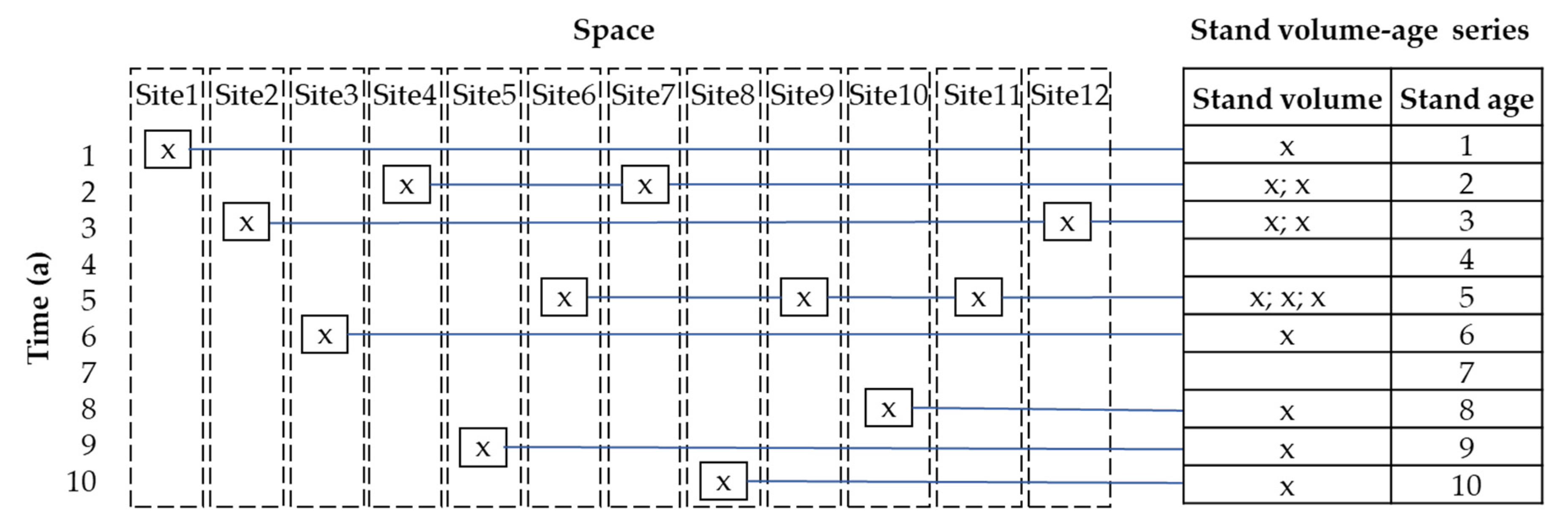
  70. Pickett, S.T.A. Space-for-Time Substitution as an Alternative to Long-Term Studies. In Long-Term Studies in Ecology; Likens, G.E., Ed.; Springer: New York, NY, USA, 1989; pp. 110–135. [Google Scholar]
  71. Ma, J.; Xiao, X.; Bu, R.; Doughty, R.; Hu, Y.; Chen, B.; Li, X.; Zhao, B. Application of the space-for-time substitution method in validating long-term biomass predictions of a forest landscape model. Environ. Model. Softw. 2017, 94, 127–139. [Google Scholar] [CrossRef]
  72. Blois, J.L.; Williams, J.W.; Fitzpatrick, M.C.; Jackson, S.T.; Ferrier, S. Space can substitute for time in predicting climate-change effects on biodiversity. Proc. Natl. Acad. Sci. USA 2013, 110, 9374–9379. [Google Scholar] [CrossRef] [Green Version]
  73. Feng, Y. The Research on Carbon Budget of Forest Ecosystem in Pu’er Region of Yunnan Province Based on CBM Model. Master’s Thesis, Chinese Academy of Forestry, Beijing, China, 2014. (In Chinese). [Google Scholar]
  74. Zeng, W.; Wang, X.; Chen, Z.; Yao, S. Analysis of impacts of forest origin on single tree biomass models. For. Resour. Manag. 2014, 40–45. (In Chinese) [Google Scholar] [CrossRef]
  75. Steinnocher, K.; De Bono, A.; Chatenoux, B.; Tiede, D.; Wendt, L. Estimating urban population patterns from stereo-satellite imagery. Eur. J. Remote Sens. 2019, 52, 12–25. [Google Scholar] [CrossRef] [Green Version]
  76. Yao, Z.; Liu, J. Models for biomass estimation of four shrub species planted in urban area of Xi’an City, Northwest China. Chin. J. Appl. Ecol. 2014, 25, 111–116. (In Chinese) [Google Scholar]
  77. Boudewyn, P.A.; Song, X.; Magnussen, S.; Gillis, M.D. Model-Based, Volume-to-Biomass Conversion for Forested and Vegetated Land in Canada; Natural Resources Canada, Canadian Forest Service, Pacific Forestry Centre: Victoria, BC, Canada, 2007.
  78. Niemand, C.; Köstner, B.; Prasse, H.; Grünwald, T.; Bernhofer, C. Relating tree phenology with annual carbon fluxes at Tharandt forest. Meteorologische Zeitschrift 2005, 14, 197–202. [Google Scholar] [CrossRef] [Green Version]
  79. Piao, S.; Friedlingstein, P.; Ciais, P.; Viovy, N.; Demarty, J. Growing season extension and its impact on terrestrial carbon cycle in the Northern Hemisphere over the past 2 decades. Glob. Biogeochem. Cycles 2007, 21, GB3018. [Google Scholar] [CrossRef]
  80. Potter, C.; Klooster, S.; Genovese, V. Net primary production of terrestrial ecosystems from 2000 to 2009. Clim. Chang. 2012, 115, 365–378. [Google Scholar] [CrossRef] [Green Version]
  81. Zhou, Y.; Zhang, L.; Fensholt, R.; Wang, K.; Vitkovskaya, I.; Tian, F. Climate Contributions to Vegetation Variations in Central Asian Drylands: Pre- and Post-USSR Collapse. Remote Sens. 2015, 7, 2449–2470. [Google Scholar] [CrossRef] [Green Version]
  82. Piao, S.; Yin, G.; Tan, J.; Cheng, L.; Huang, M.; Li, Y.; Liu, R.; Mao, J.; Myneni, R.B.; Peng, S.; et al. Detection and attribution of vegetation greening trend in China over the last 30 years. Glob. Chang. Biol. 2015, 21, 1601–1609. [Google Scholar] [CrossRef]
  83. Zhang, Q.; Qi, T.; Li, J.; Singh, V.P.; Wang, Z. Spatiotemporal variations of pan evaporation in China during 1960–2005: Changing patterns and causes. Int. J. Climatol. 2015, 35, 903–912. [Google Scholar] [CrossRef]
  84. Cui, L.; Wang, L.; Qu, S.; Deng, L.; Wang, Z. Impacts of temperature, precipitation and human activity on vegetation NDVI in Yangtze river basin, China. Earth Sci. 2019, 45, 1–24. (In Chinese) [Google Scholar]
  85. Chen, Y.; Shi, X.; Zhang, L.; Baskin, J.M.; Baskin, C.C.; Liu, H.; Zhang, D. Effects of increased precipitation on the life history of spring- and autumn-germinated plants of the cold desert annual Erodium oxyrhynchum (Geraniaceae). Aob Plants 2019, 11, plz004. [Google Scholar] [CrossRef] [Green Version]
  86. Hui, D.; Yu, C.; Deng, Q.; Dzantor, E.K.; Zhou, S.; Dennis, S.; Sauve, R.; Johnson, T.L.; Fay, P.A.; Shen, W.; et al. Effects of precipitation changes on switchgrass photosynthesis, growth, and biomass: A mesocosm experiment. PLoS ONE 2018, 13, e0192555. [Google Scholar] [CrossRef] [PubMed]
  87. Dube, O.P.; Pickup, G. Effects of rainfall variability and communal and semi-commercial grazing on land cover in southern African rangelands. Clim. Res. 2001, 17, 195–208. [Google Scholar] [CrossRef]
  88. Cao, S.; Chen, L.; Yu, X. Impact of China’s Grain for Green Project on the landscape of vulnerable arid and semi-arid agricultural regions: A case study in northern Shaanxi Province. J. Appl. Ecol. 2009, 46, 536–543. [Google Scholar] [CrossRef]
  89. Li, Z.; Chen, Y.; Li, W.; Deng, H.; Fang, G. Potential impacts of climate change on vegetation dynamics in Central Asia. J. Geophys. Res. Atmos. 2015, 120, 12345–12356. [Google Scholar] [CrossRef]
  90. Mizutani, F.; Yamada, M.; Tomana, T. Differential Water Tolerance and Ethanol Accumulation in Prunus Species under Flooded Conditions. J. Jpn. Soc. Hortic. Sci. 1982, 51, 29–34. [Google Scholar] [CrossRef] [Green Version]
  91. Crawford, R.M.M. Alcohol Dehydrogenase Activity in Relation to Flooding Tolerance in Roots. J. Exp. Bot. 1967, 18, 458–464. [Google Scholar] [CrossRef]
  92. Wang, J.; Wang, K.; Zhang, M.; Zhang, C. Impacts of climate change and human activities on vegetation cover in hilly southern China. Ecol. Eng. 2015, 81, 451–461. [Google Scholar] [CrossRef]
  93. Wimmer, R.; Grabner, M. A comparison of tree-ring features in Picea abies as correlated with climate. IAWA J. 2000, 21, 403–416. [Google Scholar] [CrossRef]
  94. Rezaei, S.A.; Gilkes, R.J.; Andrews, S.S. A minimum data set for assessing soil quality in rangelands. Geoderma 2006, 136, 229–234. [Google Scholar] [CrossRef]
  95. Mielke, L.N.; Schepers, J.S. Plant response to topsoil thickness on an eroded loess soil. J. Soil Water Conserv. 1986, 41, 59–63. [Google Scholar]
  96. Gao, S.; Yuan, X.; Gan, S.; Zhang, X. Study of the relationship between soil thickness and vegetation growth in the karst region in southeast Yunnan. Value Eng. 2013, 32, 178–179. (In Chinese) [Google Scholar]
  97. Pellissier, L.; Fournier, B.; Guisan, A.; Vittoz, P. Plant traits co-vary with altitude in grasslands and forests in the European Alps. Plant Ecol. 2010, 211, 351–365. [Google Scholar] [CrossRef] [Green Version]
  98. Hodkinson, I.D. Terrestrial insects along elevation gradients: Species and community responses to altitude. Biol. Rev. 2005, 80, 489–513. [Google Scholar] [CrossRef] [PubMed] [Green Version]
  99. McCool, D.K.; George, G.O.; Freckleton, M.; Douglas, C.L.; Papendick, R.I. Topographic effect on erosion from cropland in the northwestern wheat region. Trans. ASAE 1993, 36, 1067–1071. [Google Scholar] [CrossRef]
  100. Liu, B.Y.; Nearing, M.A.; Risse, L.M. Slope gradient effects on soil loss for steep slopes. Trans. ASAE 1994, 37, 1835–1840. [Google Scholar] [CrossRef]
  101. El-Hassanin, A.S.; Labib, T.M.; Gaber, E.I. Effect of vegetation cover and land slope on runoff and soil losses from the watersheds of Burundi. Agric. Ecosyst. Environ. 1993, 43, 301–308. [Google Scholar] [CrossRef]
  102. Kuo, T.; Liu, Z.; Li, H.; Wan, N.; Shen, C.; Ku, T. Climate and environmental changes during the past millennium in central western Guizhou, China as recorded by Stalagmite ZJD-21. J. Asian Earth Sci. 2011, 40, 1111–1120. [Google Scholar] [CrossRef]
  103. Cai, Y.; Meng, J. Ecological reconstruction of degraded land: A social approach. Sci. Geogr. Sin. 1999, 19, 198–204. (In Chinese) [Google Scholar]
  104. Damgaard, C. A Critique of the Space-for-Time Substitution Practice in Community Ecology. Trends Ecol. Evol. 2019, 34, 416–421. [Google Scholar] [CrossRef]
Figure 1. Location of Guizhou Plateau.
Forests 12 00083 g001
Figure 2. Workflow for analyzing the effect of environment factors on stand volume in Guizhou Plateau.
Forests 12 00083 g002
Figure 3. Schematic diagram of using space-for-time substitution to generate stand volume–age series.
Forests 12 00083 g003
Figure 4. Examples of using the zonal-hierarchical model method to build a set of equations. DTSG = dominant tree species (groups). Please note that the factors and stand table in the figure are hypothetical, not actual ones.
Forests 12 00083 g004
Figure 5. Workflow for growth model fitting on stand volume with application of zonal-hierarchical modeling and space-for-time substitution in Guizhou Plateau. DTSG = dominant tree species (groups), SD = standard deviation. For a detailed environmental effect analysis, see Figure 2. Please note that the factors, stand groups and stand volume–age tables in the figure are hypothetical, not actual ones.
Forests 12 00083 g005
Figure 6. Comparison between different site quality degrees in stand volume of the six selected dominant tree species (groups). The II to V in the horizontal axis denote the site quality degrees of II to V, respectively.
Forests 12 00083 g006
Figure 7. Comparison between different rocky desertification types in stand volume of the six selected dominant tree species (groups). The RD, NRD, and PRD in the horizontal axis denote the type of rocky desertification, nonrocky desertification, and potential rocky desertification, respectively.
Forests 12 00083 g007
Figure 8. Comparison between different rocky desertification degrees in stand volume of the six selected dominant tree species (groups). The SL, MD, and SV in the horizontal axis denote rocky desertification degrees of slight, moderate and severe, respectively.
Forests 12 00083 g008
Figure 9. Instances of the fitted growth curves of stand volume in Guizhou Plateau. In the title of each plot, MSH, MSSH and SSH denote the climate zones of mid-subtropical humid, mid-subtropical subhumid, and south subtropical humid, respectively; II to V denote the site quality degrees II to V, respectively; P and NS denote the plantation and natural stand, respectively; RD, NRD, and PRD denote rocky desertification, nonrocky desertification, and potential rocky desertification, respectively; and * denotes the involvement of all the classes within that factor.
Forests 12 00083 g009
Figure 10. Instances of the residuals graphs of stand volume growth models. In the title of each plot, MSH, MSSH and SSH denote the climate zones of mid-subtropical humid, mid-subtropical subhumid, and south subtropical humid, respectively; II to V denote the site quality degrees of II to V, respectively; P and NS denote the plantation and natural stand, respectively; RD, NRD, and PRD denote the type of rocky desertification, nonrocky desertification, and potential rocky desertification, respectively; and * denotes the involvement of all the classes within that factor.
Forests 12 00083 g010
Figure 11. Comparison of fitted stand volume growth curves of the six dominant tree species (groups). In the title of each plot, MSH, MSSH and SSH denote the climate zones of mid-subtropical humid, mid-subtropical subhumid, and south subtropical humid, respectively; II to V denote site quality degrees II to V, respectively; P and NS denote the plantation and natural stand, respectively; RD, NRD, and PRD denote rocky desertification, nonrocky desertification, and potential rocky desertification, respectively; and * denotes the involvement of all the classes within that factor. The legend of each plot means: CF = China fir, MP = masson pine, CY = cypress, OA = oak, CC = cyclobalanopsis, BI = birch. Please note that China fir did not have natural stand growth curves because its natural stand was very rare (gi), and cyclobalanopsis did not have a plantation in the MSH–degree II–RD forestland (j).
Forests 12 00083 g011
Figure 12. The comparison of the growth upper limit of stand volume growth equations among different dominant tree species (groups), climate zones, site quality degrees, origins and rocky desertification types. MSH, MSSH and SSH in plot (b) denote the climate zones of mid-subtropical humid, mid-subtropical subhumid, and south subtropical humid, respectively. II to V in plot (c) denote site quality degrees II to V, respectively. P and NS in plot (d) denote the plantation and the natural stand, respectively. RD, NRD, and PRD in plot (e) denote rocky desertification, nonrocky desertification, and potential rocky desertification, respectively.
Forests 12 00083 g012
Figure 13. Correlation between the years of growth slowing down and growth upper limit of stand volume.
Forests 12 00083 g013
Table 1. Explanation of the environmental factors.
FactorsUnitClassificationRange/CategoriesNotes
Temperature°CContinuous6.95–21.67Mean annual temperature in 2016, accurate to 2 decimal places
PrecipitationmmContinuous832.11–1994.77Sum annual precipitation in 2016, accurate to 2 decimal places
Stand origin--CategoricalNatural stand; PlantationWhether a stand grow up naturally or by cultivated
ElevationmContinuous145–2900The height above sea level, accurate to integer
Slope gradient°Continuous1–90The degree of slope, accurate to integer
Aspect--CategoricalNorth; Northeast; East; Southeast; South; Southwest; West; Northwest; FlatThe direction in which the normal of a slope is projected onto a horizontal plane, was divided into 9 classes.
Slope position--CategoricalRidge; Upper slope; Middle slope; Lower slope; Valley; Flat ground; All slopeThe geomorphic part located in a slope, was divided into 7 classes.
Topsoil thicknesscmContinuous1–115Sum of the thickness of A horizon and B horizon, accurate to an integer.
Site quality degree--OrdinalI (removed); II; III; IV; VThe degree from I to V represents the site quality from high to low. As the forestland denoted by degree I in the study area were very rare and cannot provide sufficient samples, we remove it in the following analysis.
Rocky desertification type--CategoricalRocky desertified (RD); Potential rocky desertified (PRD); Nonrocky desertified (NRD)RD refers to the stands with ≥ 30% bedrock exposed and < 50% vegetation-covered; PRD refers to the stands with ≥ 30% bedrock exposed and ≥ 50% vegetation-covered; NRD refers to the stands with < 30% bedrock exposed.
Rocky desertification degree--CategoricalSlight; Moderate; Severe; Extremely severe (removed)Only those stands denoted by RD and PRD have a value of rocky desertification degree. The land extremely severe desertified could hardly grow any vegetation so we remove it in the following analysis.
Table 2. The total stand volume and proportion of the 36 categorized dominant tree species (groups) in the Guizhou Plateau in 2016.
NoDominant Tree Species (Groups)Canopy DensityStand Age(a)Stand DBH
(cm)
Stand Height
(m)
Total Stand Volume
(103 m3)
Stand Volume
(m3 ha−1)
SD of Stand Volume
(m3 ha−1)
1Fir0.5919.9614.379.1029.2856.4442.44
2Spruce0.5219.5212.048.6629.6947.3337.65
3Chinese yew0.126.032.352.1815.033.8924.28
4Masson pine0.5521.8915.7811.72135,847.7080.6558.14
5Huashan pine0.5922.1514.278.8510,356.2165.9453.41
6Yunnan pine0.6124.3712.808.4811,993.1869.0842.14
7Other pine0.5012.9210.327.56740.6147.8251.85
8Keteleeria0.5526.8015.018.33195.6451.8941.87
9Hemlock0.6140.8920.8710.934.0943.2525.55
10Cypress0.4820.6710.358.1012,000.3137.0631.62
11Other cypress0.3914.536.925.91931.5723.1834.20
12China fir0.4815.2010.998.4913,8317.3581.5970.49
13Cryptomeria0.5613.7211.048.3211,964.1470.8366.02
14Metasequoia0.6215.0611.589.1184.0248.3751.90
15Other fir0.5323.2013.708.5469.3451.7752.01
16OCTS 10.5522.2613.939.2186.7643.7365.58
17Poplar/aspen0.4814.6812.6510.392698.1133.6832.32
18Willow0.369.908.016.1618.2022.1240.68
19Eucalyptus0.536.749.0510.202747.7761.0646.50
20Camphor0.4915.3510.207.26313.1132.5535.38
21Phoebe0.4522.7912.158.70187.7160.5940.67
22Oak0.5618.629.977.697990.9936.2429.96
23Cyclobalanopsis0.5112.738.908.429732.5245.8327.63
24Beech0.5416.2112.319.01180.9562.5427.54
25Birch0.5014.7511.028.955786.6732.5125.81
26Basswood0.6533.5516.8411.696.9632.6544.47
27Locust0.4822.1612.869.03702.9637.4335.65
28Katus0.5017.5315.4110.48933.5953.8329.10
29Maple0.4618.0316.0911.98127.4675.4730.09
30Melia0.5720.2811.949.30122.9938.3434.35
31Chinese toon0.6331.7416.2311.39814.7638.3138.94
32Elm0.5521.6314.5710.43255.8729.4123.73
33Ebony0.5522.1812.029.4956.8272.7230.75
34Firmiana0.4620.2019.6712.46206.5538.5635.03
35OBTS 20.5219.0111.879.4769,078.9841.4535.46
36BMTS 30.5521.1911.899.2227,841.3658.7138.15
Note: Canopy density, stand age, stand DBH, stand height and stand volume were the average values of all related stands, and the SD of stand volume was the standard deviation of stand volume (per hectare) of all related stands. 1 OCTS = Other coniferous tree species (groups); 2 OBTS = Other broad-leaved tree species (groups); 3 BMTC = Broad-leaved mixed tree species (groups).
Table 3. Statistics of the correlation analysis between stand volume of the six selected dominant tree species (groups) and temperature, precipitation, elevation, slope gradient, and topsoil thickness. Slope is the slope of the regression line, and Spearman’s ρ is the Spearman rank correlation coefficient.
Environmental FactorsDominant Tree Species (Groups)SlopeSpearman’s ρp-Value
TemperatureChina fir12.760.2838<0.0001 **
Masson pine0.290.00510.3366
Cypress−0.65−0.01730.5520
Oak−1.59−0.1023<0.0001 **
Cyclobalanopsis2.030.1543<0.0001 **
Birch5.380.2569<0.0001 **
PrecipitationChina fir0.130.2833<0.0001 **
Masson pine−0.01−0.03050.5409
Cypress0.010.05100.0373 *
Oak−0.01−0.09210.0036 **
Cyclobalanopsis0.020.07290.0214 *
Birch0.070.1742<0.0001 **
ElevationChina fir−0.05−0.2453<0.0001 **
Masson pine−0.005−0.01010.2422
Cypress0.010.06210.0863
Oak0.010.1309<0.0001 **
Cyclobalanopsis−0.01−0.07160.0236 *
Birch−0.02−0.1702<0.0001 **
Slope gradientChina fir−0.51−0.05450.0267 *
Masson pine−0.42−0.05150.0448 *
Cypress−0.15−0.04300.1745
Oak−0.60−0.2921<0.0001 **
Cyclobalanopsis−0.38−0.11290.0097 **
Birch−0.43−0.1235<0.0001 **
Topsoil thicknessChina fir0.840.2652<0.0001 **
Masson pine0.580.1958<0.0001 **
Cypress0.250.13910.0024 **
Oak0.220.1668<0.0001 **
Cyclobalanopsis0.370.2202<0.0001 **
Birch0.280.14440.0002 **
Note: the * symbol on the top-right of the p-value means the correlation is significant (p < 0.05), while ** symbol means the correlation is very significant (p < 0.01).
Table 4. Statistics and p-value of the Wilcoxon rank-sum test of stand volume of the six selected dominant tree species (groups) between different stand origin types. Mean, SD and CV represent the mean value (m3 ha−1), standard deviation (m3 ha−1), and coefficient of variation (%) of the specific tree species.
Dominant Tree Species (Groups)Natural StandPlantationWilcoxon Test p-Value
MeanSDCVMeanSD CV
China fir141.971.3450.28--------
Masson pine95.2857.0659.88112.958.751.990.0007 **
Cypress55.625.6446.1251.6132.0662.110.0009 **
Oak 42.930.4871.0458.9932.1154.430.0030 **
Cyclobalanopsis64.7537.0857.2763.8634.7954.480.8700
Birch 51.4934.3866.7662.2139.9264.180.0040 **
Note: the ** symbol on the top-right of the p-value means the correlation is very significant (p < 0.01).
Table 5. Statistics about the significance of the correlation between stand volume of the six dominant tree species (groups) and environmental factors. The sum column equals to the number of dominant tree species (groups) denoted by the * symbol and the ** symbol, and the rank column is the rank of environmental factors according to the significance of their correlation with stand volume, the higher sum value and the more ** symbols, the higher the rank is.
Environmental FactorsChina FirMasson PineCypressOakCyclobalanopsisBirchSumRank
Temperature** ******46
Precipitation** ******53
Stand origin--****** **45
Elevation** *****48
Slope gradient** ******53
Aspect ** *210
Slope position ** 111
Topsoil thickness************61
Site quality degree***********62
Rocky desertification type**** ** **46
Rocky desertification degree ** ** 39
Sum8651079----
Note: the * symbol on the top-right of the p-value means the correlation is significant (p < 0.05), while the ** symbol means the correlation is very significant (p < 0.01).
Publisher’s Note: MDPI stays neutral with regard to jurisdictional claims in published maps and institutional affiliations.

