Article

Is Soil Contributing to Climate Change Mitigation during Woody Encroachment? A Case Study on the Italian Alps

1
Sogesid s.p.a c/o Italian Ministry for the Environment, Land and Sea (MATTM) Via Cristoforo Colombo, n. 44, 00147 Rome, Italy
2
Department for Innovation in Biological, Agro-food and Forest systems (DIBAF), University of Tuscia, Via San C. De Lellis snc, 01100 Viterbo, Italy
3
Foundation Euro-Mediterranean Center on Climate Change (CMCC), Division on Impacts on Agriculture, Forests and Ecosystem Services (IAFES), Viale Trieste 127, 01100 Viterbo, Italy
4
Istituto di Servizi per il Mercato Agricolo Alimentare (ISMEA), Viale Liegi 26, 00198 Rome, Italy
5
Department of Landscape Design and Sustainable Ecosystems, Agrarian-Technological Institute, RUDN University, Miklukho-Maklaya str., 6, 117198 Moscow, Russia
*
Author to whom correspondence should be addressed.
Forests 2020, 11(8), 887; https://doi.org/10.3390/f11080887
Submission received: 12 June 2020 / Revised: 10 August 2020 / Accepted: 12 August 2020 / Published: 15 August 2020
(This article belongs to the Section Forest Ecology and Management)

Abstract

:
Background and Objectives: Over the last few decades, the European mountain environment has been characterized by the progressive abandonment of agro-pastoral activities and consequent forest expansion due to secondary succession. While woody encroachment is commonly considered as a climate change mitigation measure, studies suggest a still uncertain role of the soil organic carbon (SOC) pool in contributing to climate change mitigation during this process. Therefore, the objective of the study is to investigate the possible SOC variations occurring as a consequence of the secondary succession process at the provincial level in an Alpine area in Italy. Materials and Methods: A chronosequence approach was applied to identify, in five different study areas of the Belluno province, the land use/land cover change over four different stages of natural succession, from managed grazing land to secondary forest developed on abandoned grazing land. In each chronosequence stage, soil samples were collected down to the bedrock (0–60 cm depth) to determine the changes in the SOC stock due to the woody encroachment process. Results: In all areas, small or no significant (p < 0.05) SOC stock changes were observed during the secondary succession in the upper 30 cm of mineral soil, while significant changes were evident in the 30–60 cm compartment, with the SOC stock significantly decreasing from 30% to 60% in the final stage of the succession. This fact indicates the great importance of considering also the subsoil when dealing with land use/land cover change dynamics. Conclusions: The recorded trend in SOC has been proved to be the opposite in other Italian regions, so our results indicate the importance of local observation and data collection to correctly evaluate the soil contribution to climate change mitigation during woody encroachment.

Graphical Abstract

1. Introduction

Natural capital, climate change, and ecosystem services availability are strictly connected to the soil quality and land-use change (LUC) dynamics around space and time [1]. To face new challenges in land degradation, most of the Multilateral Environmental Agreements indications have been translated into the United Nations Sustainable Development Goals (SDGs), addressing target definition and reframing agricultural and environmental policies at a different scale, from macro to local [2]. In that multilevel worldwide policy definitions process, the management of abandoned land could represent a crucial point for the climate change mitigation potential of agriculture and forestry activities, and particularly the role of the soil organic carbon (SOC) pool [3,4,5]. This issue is also recognized in the European Thematic Strategy for Soil Protection [6], and recalled in the new Green Deal European Commission proposal [7], where it was defined that the maintenance of SOC stocks is essential for the fulfilment of present and future emission reduction commitments at the European level. The 2019 Intergovernmental Panel on Climate Change (IPCC) Special Report on Climate Change and Land emphasizes that meeting the Paris Agreement’s temperature goal will not be possible without radical changes in how land resources are utilized [1]. The 2030 European Union (EU) climate and energy policy framework includes a dedicated instrument concerning greenhouse gas (GHG) emissions and removals from land use; land-use change and forestry (LULUCF); and the LULUCF Regulation 2018/841 [8], where the SOC is considered as one of the five ecosystem C pools that should be reported and accounted for in managed land, especially in the case of LUC. Whether abandoned land falls in the domain of “managed land” and can thus be included in the national GHG balance depends on the local laws and regulations in each country. Nevertheless, in general, the whole territory of the EU can be considered as “managed”, as it is somehow subject to human activities, policy, and measures (e.g., fire protection, land planning, protection policies, or recreation).
Although the role of the SOC is well recognized in the European context, currently there are no specific binding laws and actions for soil protection that are often integrated in different sectorial and environmental policies (e.g., Natura 2000 network; Water Framework Directive) [9]. Actually, soil protection is pursued through partial specifications in the European Common Agricultural Policy (CAP) framework, where a farmer’s payment/subsidy is conditional on compliance with some standards concerning soil management (e.g., cross-compliance), land use, and management (e.g., greening) [10,11]. Besides, in the second pillar, CAP provides voluntary agro-climate-environmental schemes financed by the European Agricultural Fund for Rural Development (EAFRD) to improve soil quality, as reported in priority 4—“restoring, preserving and enhancing ecosystems related to agriculture and forestry”—identifying a specific focus areas dedicated to preventing soil erosion with the 1305/2013 EU regulation [12]. The active management of these marginal territories could be considered a strategy for both climate change mitigation and soil protection in marginal mountain areas.
Land abandonment and the consequent woody encroachment is an extensive phenomenon in European mountain territories and, particularly, in the Mediterranean area [13,14,15]. The woody encroachment process occurring in marginal lands causes a natural LUC, which is responsible for a shift in land cover, causing profound changes in the structure of the ecosystem and in the fluxes of C connected with the different ecosystem C pools [16]. Apart from an obvious increase in the C stored in the biomass (both aboveground and belowground) as a result of the change in vegetation, the woody encroachment process may have a dissimilar impact on the SOC pool as a function of the considered LUC [17,18], with clear and significant SOC stock increment when occurring on cropland, and highly variable effects over managed or unmanaged grasslands [17,18,19,20,21]. In the case of grasslands, the main reason for this variability can be related to several parameters and their combination. A significant role in driving the direction of the SOC stock changes along the woody encroachment process is played by the forest types (conifers vs. broadleaves) [17,19] and the site’s climatic conditions, mainly mean annual precipitations and mean annual temperatures [17,18,19,20,21]. As woody encroachment begins, lands undergo profound changes in species composition, patch-type diversity, and microclimate [19,22]. Besides, the shift toward forest can change the soil fauna composition in favor of species less capable of transferring the C inputs (e.g., litter deposition) into the mineral soil [23,24], particularly in conifer-dominated secondary forests. In the most dramatic situations, these changes can cause a SOC depletion, which is usually overturned by the C accumulated in the organic layer [25,26] and aboveground biomass [27]. Although some studies do not clearly indicate soil as a major C reservoir contributing to climate change mitigation trough SOC sequestration along this natural land use change [17,18,20,22,26], some others suggest a major role of the soil compartment [3,4,5,19,28]. This fact indicates the importance of understanding the role of the soil to act as a C sink or source with respect to the woody encroachment process to correctly define future politics aimed at increasing C sequestration by terrestrial ecosystems. The LULUCF regulation poses also a new challenge to EU Member States that will need to report, starting from 2023, on the basis of a spatial explicit approach that implies that the land parcels where LUC occurs need to be identified and the GHG emissions and removals tracked, thus giving the opportunity to characterize the GHG fluxes with local specific factors.
Based on these premises, the aim of this study was to quantify the SOC changes due to the natural succession toward forest occurring on abandoned grazing land in the Italian Alps, in the Belluno province. This aim is justified by the increasing European area affected by land abandonment and the possible contribution to climate mitigation offered by the SOC pool in connection with the orientation of agricultural land management policies in mountain rural areas under the Common Agricultural Policy.

2. Materials and Methods
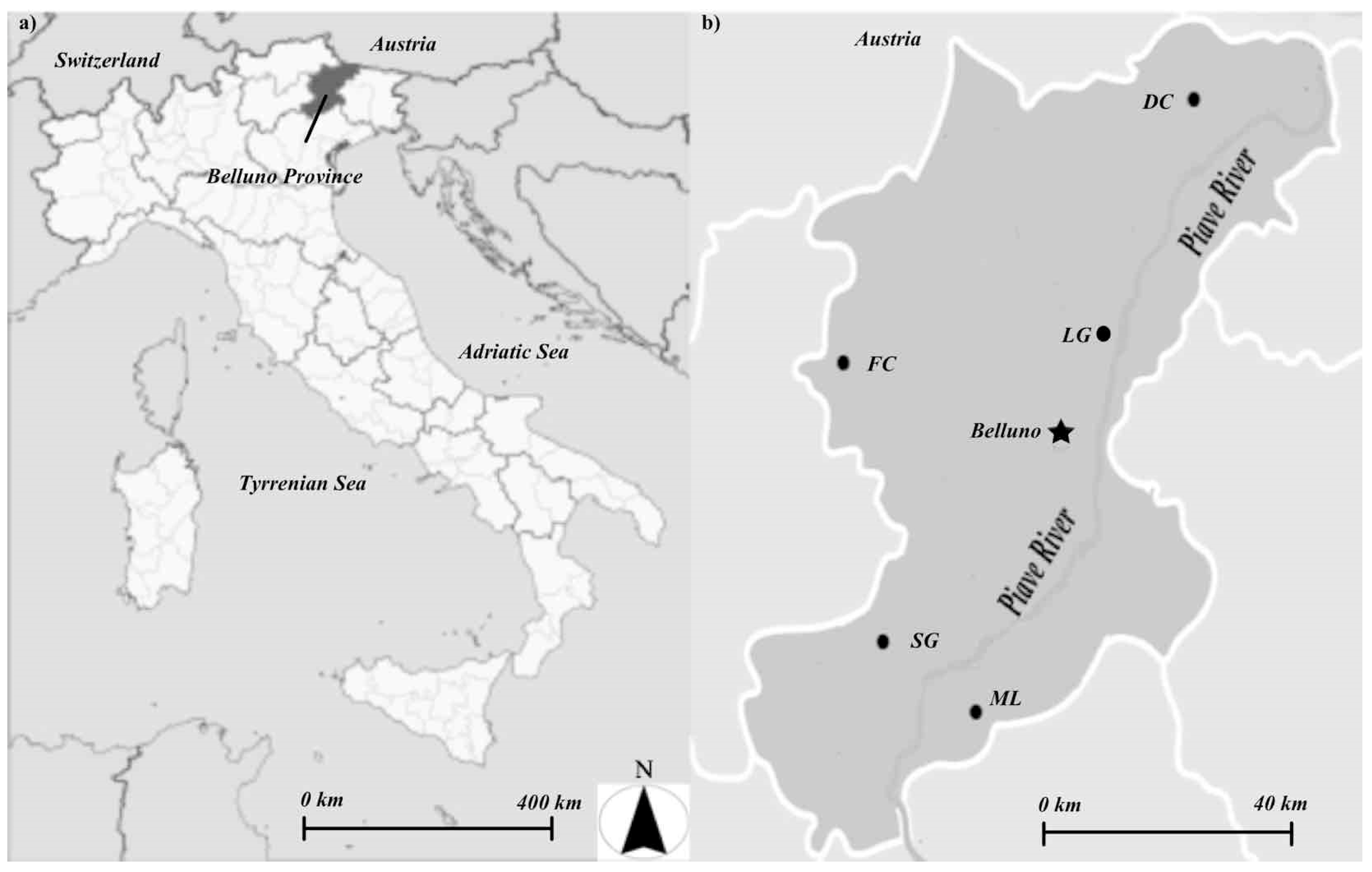
2.1. Study Area

The study sites are located in the Belluno province, Veneto Region, Italy (Figure 1a,b). The climate of the province is typical of the Alpine regions, with a mean annual temperature of 10 °C and a mean annual precipitation of about 1200 mm (www.arpa.veneto.it), which varies in the different areas of the province according to altitude and location (Table 1). The province entirely coincides with part of the Piave river basin. The territory constitutes 81% agricultural and forestry areas. The province is a typical Alpine province, with scarce arable lands and an abundance of permanent grazing lands, meadows, shrublands, and forests. The main soil types are comprised within the order of Cambisols and Phaeozems [29], and are usually shallow on the mountain slopes and moderately deep in the valley bottom [30].

2.2. Experimental Design

To evaluate the changes in SOC caused by woody encroachment, we used a chronosequence approach which corresponds to the so-called space-for-time substitution suggested by Walker et al. [31]. Therefore, we identified, in a close range, a set of spatially separated areas, similar for exposure, slope, and elevation, but different for recent land use and land cover history, which represent stages encroached in different periods over time. These areas were subjected to a synchronic analysis in the field. We identified five chronosequences (hereafter called sites) from different municipalities of the Belluno province: Danta di Cadore (DC), Falcade (FC), Longarone (LG), Mel (ML), and Santa Giustina (SG) (Figure 1b). In each site, we selected a pasture currently managed to represent the starting point of natural succession (T0). In order to define the land use patterns over time, all the T0s were identified using the beneficiary lists of the Rural Development Programme (RDP) measure for the maintenance of grasslands (measure 214/e) of the Veneto RDP funds [32], which concerned all sites since 2013. By combining the use of airborne digital orthophoto series from 1988 to 2009, interviews with local farmers, and the beneficiary list of the RDP measure for the restoration of grasslands affected by woody encroachment (measure 216-6) of the Veneto RDP [32], it was possible to individuate three more stages of the succession: (1) abandoned grazing land at the initial stage of the succession, with herbaceous vegetation and shrubs (T1); (2) abandoned grazing land at an intermediate stage, with abundant woody vegetation and shrubs (T2); and (3) abandoned pasture at an advanced stage of the succession, with the forest canopy closed (T3). In summary, 5 sites with 4 stages each were individuated. On the basis of the previous data sources and combining areal images with interviews with local farmers, we were able to assign an approximate abandon age to each of the stages: 15 years for T1, 35 years for T2, and around 70 years for T3 (A1–A5). The vegetation species of each stage from the different chronosequences along with the information on the age of the stage and the size of the area covered by the stage are reported in Table A1, Table A2, Table A3, Table A4 and Table A5. In each site, the chosen stages were located close to each other, with 500 m being the maximum distance.

2.3. Sampling Strategy and Soil Analyses

The protocol proposed by the European Commission [33] to determine SOC variations as a consequence of a land-use change was selected for the soil sample collection. The protocol is based on a pseudorandom selection of three plots in each successional stage. Following the protocol, the dimensions of the plots were determined according to the dimension of the area covered by each successional stage [33]. In addition to the recommendation suggested for this protocol application [34], in this study we made an implementation considering the whole soil profile to the bedrock and not only the 0–30 cm layer. In particular, the sampling was performed in the topsoil at 0–5, 5–15, and 15–30 cm depths and in the subsoil at 30–45 and 45–60 cm depths. In each of the plots, soil samples were collected by means of an auger in 25 points distributed on the basis of a 5 by 5 sampling grid according to the ISO 10381-4 standard [35]. The 25 samples collected per plot and layer were mixed in the field to have one composite sample to be used for the analyses. Considering the three plots, there were three composite samples per depth in each chronosequence successional stage. In the center of each plot, a trench was opened to a 40 cm depth and used to collect bulk density (BD) samples using a known volume (98.1 cm3) metal cylinder according to Blake [36] for the depths comprised in the topsoil. When present, the organic horizon was collected within a frame of 40 by 40 cm randomly positioned in each plot to obtain three replicates per stage. In summary, 5 sites with 4 stages each were sampled. In each stage, 3 sampling plots were considered and, for each of them, a composite sample (based on 25 subsamples) was collected for each layer (5 depth intervals). Overall, 480 soil samples were collected (300 for soil and 180 for BD).
All the samples were oven-dried (60 °C) to a constant mass. The organic horizon was ground in a ball mill, while the mineral soil was sieved at 2 mm and the chemical analyses were performed on the fine earth fraction (<2 mm). The particle size distribution was determined by the pipette method, while the pH was measured in a 1:2.5 soil/water suspension using a pH meter electrode [37]. The total C was measured on finely ground samples by dry combustion (Thermo-Finnigan Flash EA112 CHN, Okehampton, UK). The SOC stock (in kg C m2) of the i soil layer was calculated for each depth according to Poeplau et al. [38] and Hobley et al. [39]:
SOCstock i = SOCconc fine   soil BD sample depth i ( 1 Rock mass ) ,
where SOCconcfine soil is the organic C concentration of the fine earth (g C kg−1 soil), BDsample is the apparent soil bulk density (g soil cm−3), depthi is the depth of investigated (i) soil layer (cm), and the Rockmass is the rock fragments fraction in mass percentage (mass%/100). The SOC stock estimates were, then, converted into Mg C ha−1. For the two layers comprised in the subsoil compartment, the BD was estimated using the pedotransfer function proposed by Adams [40]:
B D =   1 ( a + b % C ) ,
where a and b are two constant values (0.686 and 0.085, respectively) suggested by Chiti et al. [41] for deep soil layers, and %C is the SOC percentage. In line with the IPCC guidelines [42], the changes in the SOC stock were reported for the topsoil (0–30 cm) and, to have an indication of the contribution from the subsoil, the changes were reported also down to the bedrock (30–60 cm).

2.4. Statistics

The C concentration and C stock of the different soil layers were tested for normality and homoscedasticity using Anderson–Darling and Levene’s tests [43], respectively. The differences in the means of the C concentration and C stock between stages were tested for significance using a one-way analysis of variance (ANOVA) between different stages, incorporating repeated measures. A post-hoc Tukey’s test at p < 0.05 was used, whenever necessary, to reveal significant differences among the mean values. The entire statistic was implemented using the R software [44].

3. Results

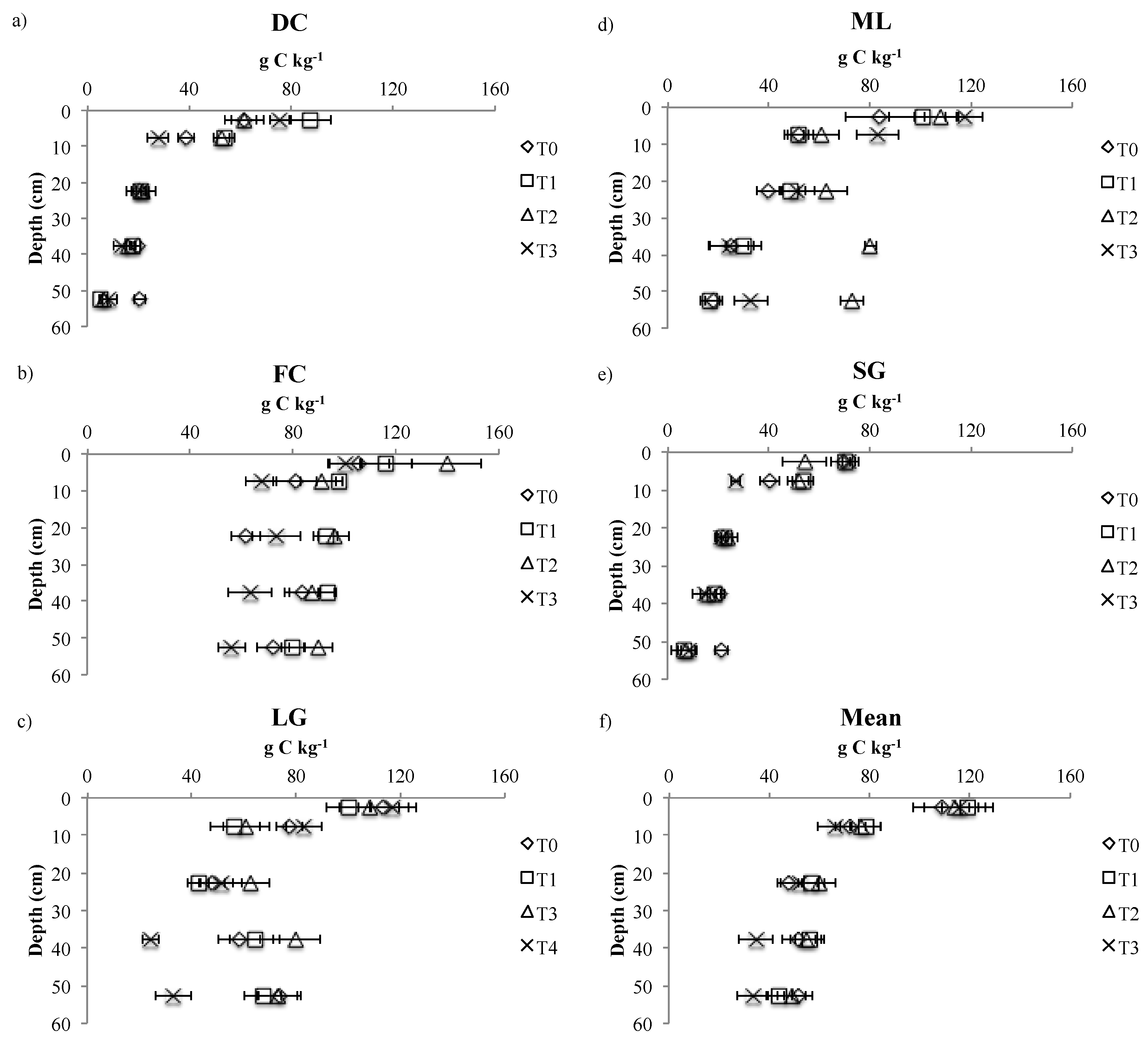
3.1. Soil Physical and Chemical Parameters

The similarity of the main physical (i.e., particle size distribution) and chemical parameters (i.e., pH) between the stages of each chronosequence assured site comparability, while some differences were observed between different areas (Table A6 and Table A7). In the different areas, the particle size distribution varied from loam (DC, SG) to clay-loam (FC, LG) and silty clay-loam (ML). Concerning the pH, no significant variations were observed between the same layer in the different stages of each chronosequence. The bulk density increases with depth within a stage, but non-significant differences were observed from the T0 to the T3 stages within the same area (Table A8). In terms of rock fragments, we observed a general higher content in mature forest (T3) stages than in the corresponding grazing lands, possibly explained by the fact that those sites were the first to be abandoned, the presence of stones being higher and the sites being basically less productive (Table A8). In terms of SOC concentration, within each stage there is a gradual decrease with depth. The comparison of the same stage from different sites reveals significant differences, particularly in the 0–5 cm layer, with grazing land (T0) showing values ranging from 61.3 ± 5.0 (DC) to 113.6 ± 9.7 g C kg−1 (LG). The same variability is evident for the T3 stage, with values ranging from 71.7 ± 2.5 (SG) to 117.3 ± 8.8 g C kg−1 (LG) (Figure 2; Table A9). The lowest SOC concentration values in all the layers are always in the DC and SG sites, with the Cambisol and Phaeozem soil types, respectively. ML is the only site where the SOC concentration does not show any statistical differences among the stages in each layer. In the other sites, significant changes in SOC concentration occur without any apparent common trend in the topsoil layers, while in the subsoil layers (30–45 and 45–60 cm) the T0 stages are always characterized by higher SOC concentrations (generally between 10% and 60%) than those of the T3 ones (Figure 2; Table A9).

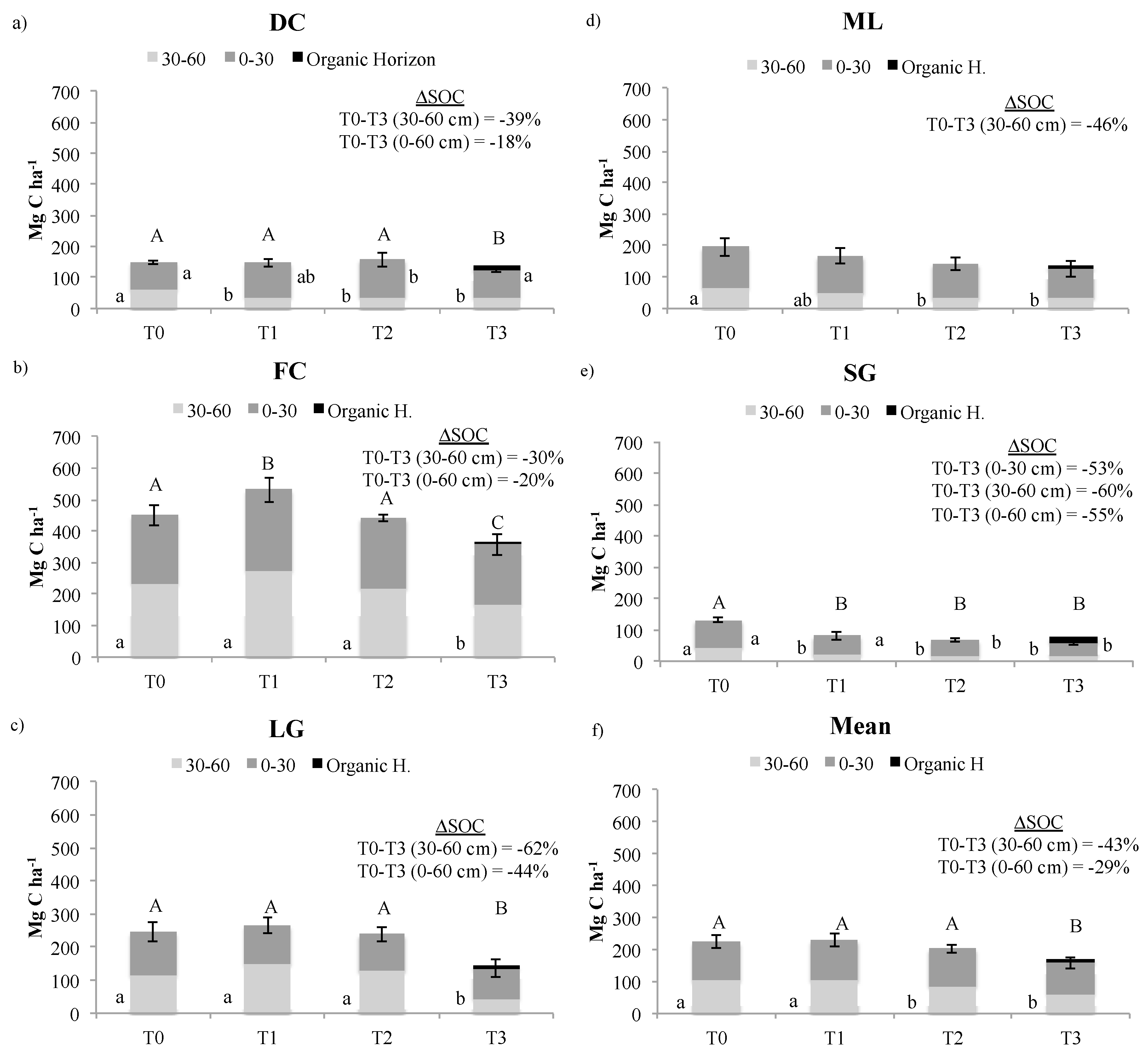
3.2. SOC Stocks Changes

Considering the topsoil (0–30 cm interval), no significant changes in SOC stock occur over time, from T0 to T3, in the LG, FC, and ML sites. In DC, a significant increase was observed in the T2 intermediate stage, while in SG a significantly lower SOC stock was estimated in the T2 and T3 stages, with a SOC stock loss of more than 50% of that estimated for T0 (Figure 3 and Table A10).
Most of the changes were observed in the subsoil (30–60 cm layer), with the SOC stock significant decreasing from the T0 to the T3 stage in all the sites. The T3 stage shows on average an SOC stock 39% (DC), 30% (FC), 62% (LG), 46% (ML), and 60% (SG) lower than the T0 stage (Figure 3).
Taking into consideration the whole soil profile (0–60 cm), except in the ML site where no significant SOC changes were estimated, the loss of SOC in the final T3 stage ranges from 10% in DC to 55% in SG. Considering the mean SOC stock from all sites (Figure 3f), in the 0–30 cm layer the SOC stock significantly decreases only in the T3 stage, while in the 30–60 cm layer the decrease is significant already in the T2 stage. Considering the whole profile, the trend is identical to that of the topsoil. The organic horizon, which is present only in the final forest stage, shows a C stock ranging from 7.0 ± 1.4 (FC) to 20.7 ± 6.3 Mg C ha−1 (SG) (Figure 3, Table A10).

4. Discussion

4.1. Impact of Land Abandonment on the SOC Pool

Temperatures [19,20] and precipitations [18,21,45] are thought to be the main determinants for the SOC changes occurring after land abandonment and woody plant invasion on grazing lands. The estimated SOC stock changes between managed grasslands (T0 stage) and encroached forest stages (T3) do not show any statistical correlation, nor mean annual temperature, nor mean annual precipitation (data not shown). However, the small range of values, especially for the precipitation parameter (1224–1483 mm yr−1), can justify the absence of these correlations.
According to an Italian study by Alberti et al. [45], 900 mm of mean annual precipitation represents the threshold for SOC changes, with the SOC levels decreasing in areas of high precipitation (>900 mm yr−1) and increasing in areas with low precipitation. Our results for the Belluno province, with an average precipitation of about 1200 mm, are in line with the literature, showing that grazing land abandonment generally leads to a SOC stock decrease. However, this decrement is evident only considering the whole profile (0–60 cm) rather than considering the topsoil (0–30 cm), where no changes were observed. This fact indicates the great importance of considering also the subsoil when dealing with LUC dynamics, as was observed also by Poeplau et al. [20] for temperate zones and by Pellis et al. [19] in different mountain areas of Italy. This is mainly explained by the fact that the C vertical distribution along the profile depends not only on the soil characteristics (e.g., pedological class, texture) but also on the climate parameters [21] and vegetation types [19]. Forest canopy closure may alter the microclimatic conditions, reducing the summer temperature in comparison to open grasslands, thus reducing the organic matter decomposition rate [46]. This fact implies, as observed, in the forest stages, an aboveground litter accumulation in the organic layer, which is very small or not present in grazing land. In addition, conifers, which dominate the investigated forest stages, can produce a more recalcitrant and slowly decomposable litter compared to herbaceous vegetation [47,48]. Besides, conifer forests are generally characterized by a reduced presence of grasses and understory vegetation, which produce highly palatable dead organic matter [49]. These conditions generally reduce soil pH with respect to grazing land and inhibit heartworm activity and their vertical organic matter translocation [24,50]. In this study, the pH (Table A6 and Table A7) does not show any significant variation in soil acidity, probably because the forest stages are not old enough to significantly affect this parameter. Finally, Puhe [51] noticed that conifer fine roots, which are affected by a rapid turnover, are mainly limited to the upper 10 cm of depth. Therefore, the main (above- and below-ground) litter deposition in the upper soil part, with the alteration of the microclimate conditions, supports our results of an SOC stock reduction in the subsoil compartment during the woody encroachments process.
Organic horizons are present only in the mature forest stages (T3), and the C stored in this compartment is not enough to offset the sizable, even if not always significant, mineral soil C losses. Similar to this study, Thuille et al. [52], Thuille and Schulze [26], Alberti et al. [17], and Guidi et al. [22] observed a SOC decrease from the mineral layers due to forest expansion in abandoned grazing lands on the Italian Alps, despite some studies that also reported no changes or even an increase in the SOC stocks in montane areas of Spain [53], Switzerland [27], and Italy [19]. In this regard, the trend in SOC emission/reduction can vary greatly depending on the pedo-climatic conditions, but currently no site-specific data collection programs are present to characterize the different pedo-climatic situations [54].
Looking at the C stored at an ecosystem level allows for a better understanding of the mitigation potential due to woody encroachment into abandoned grazing lands. A study performed in one of the sites considered in this study (the ML site) by Pellis et al. [19] indicates that the C stock in the aboveground biomass of grazing land (T0) was 0.2 Mg C ha−1, while the belowground C pool was about 13 Mg C ha−1. On the contrary, in mature forests (T3) the aboveground biomass was 156 Mg C ha−1 and the belowground C pool was about 30 Mg C ha−1. Besides, the C in the organic horizon pool, ~10 Mg C ha−1, and that in the deadwood C pool, ~3 Mg C ha−1, need to be considered also [19]. Hence, looking at the process of woody encroachment at an ecosystem level, it is evident that the C sink effect of the growing living biomass (above and below ground) and the deadwood and organic horizon C accumulation overturn the C losses observed for the soil compartment. On the basis of the previous data, we suppose that, in the investigated area, the woody encroachment can have a mitigation potential ranging from 70 (LG) to 160 Mg C ha−1 (ML and DC). In other montane areas of Italy (e.g., along the central and southern Apennines), the mitigation potential is much higher, ~300 Mg C ha−1 [18,26], mainly due to the increase in SOC, with about 45% more SOC in forestland (T3) than in grazing land (T0). Considering climate change mitigation, in the long term a forest ecosystem can accumulate a greater amount of C than grazing lands and transitional phases. The main concern is the time needed by the natural succession to be completed—at least 70–100 years [19,28] in the Italian territory or longer, even more than 150 years, in temperate forests [20]. Besides, during the succession most of the C is stored in tree biomass and organic layers, which constitute less stable C pools due to external disturbances (e.g., management, harvesting, and environmental modifications), compared with the C stored in the mineral soil layer.

4.2. Implication for Rural Development Programmes and Climate Policies

The abandonment of agricultural activity and natural reforestation phenomena are very diffuse in most of the Alpine territories [55]. The Rural Development Programmes (RDPs) are the main tools for the allocation of the European Agricultural Funds for Rural Development, where the preservation of soil against erosion and the improvement of soil management are identified as key priorities (priority 4). Many RDPs identify that the loss of grazing lands, located on shallow soil on steep slopes, can lead to an increase in hydrogeological risk and erosion, in addition to the serious compromise of historic rural landscapes and, lastly, the loss of biodiversity that characterizes mountain open spaces [56,57]. In Italy, regional administrations are in charge of designing the RDP, and within the Veneto Region RDP objectives, the Alpine landscape and environment are identified as focus area for intervention. Coherently with the general trend over the Alps, the forest area in the Belluno province increased up to 20% and agricultural lands decreased by 40% from 1980 to 2000 [58]. To enhance agroforestry practice adoption and to safeguard alpine biodiversity habitat, in 2013 the Belluno province financed 87 projects devoted to mountain grazing land restoration measures under the RDP (measure 216-6) and involving about 600 hectares of interventions [59]. In the current RDP programming for the period 2013–2020, similar landscape restoration actions are promoted [60]. The implementation of such measures implies that, for the Veneto Region, over 1000 ha are currently affected by the woody encroachment process.
The climate change mitigation potential is only one of the different ecosystem services provided by grazing lands; nevertheless, its quantification can be helpful for co-defining different policies using a multiple-criteria decision analysis approach [61]. The results from this study could be used by the Veneto Region to better assess the effect of grazing land restoration measures considering the focus area “e” objectives (fostering C conservation and sequestration in agriculture and forestry).
Besides, at the European level the LULUCF sector is increasingly playing a key role also in the climate policy framework. The decision of the European Commission, n. 529/2013/EU [62], required Member States to report the emissions and removals of GHG resulting from LULUCF activities, though not contributing to the EU 2020 objectives. With the recently approved LULUCF regulation for the post-2020 period [8], the sector’s emissions and removals are allowed to contribute towards the EU 2030 policy framework target, although with some limitations [63]. Both systems (current decision and future regulation) make mandatory, among other things, the accounting and reporting of emissions and removals in grazing land, cropland, and managed forests, as well as emissions and removals due to conversions from and to forestland. Data from the European National Inventory Report show that the LULUCF sector is responsible for a net sink of –255 810 GgCO2eq (69 766 GgC) in 2018 (EU27 + Iceland and UK), with an increasing trend from 1990 mainly due to the natural expansion of grazing land and forestland [64]. Similarly, in Italy the sink in the LULUCF sector is increasing at an average of about 237 GgC per year [65]. Between 1998 and 2017, the conversion of 1.3 million ha from grazing land to forestland led to a sink of 1161 Gg C yr−1, of which 238 Gg C yr−1 is attributed to the SOC pool (data related to 2017). Nevertheless, in the National GHG Inventory, the estimation of SOC due to conversion from grazing land to forestland is based on a single grazing land default value of SOC for the whole Italian territory (SOC0–30 cm = ~79 Mg C ha−1), while for forest soils six values for the 0–30 cm depth are used for different time periods, ranging from ~80 to 82 Mg C ha−1, thus always implying an increase in the C content in land that is converted from grazing land to forest. The coarse representation of the SOC changes is due to a lack of specific studies and a lack of detailed information about the location where the LUC occurs, which is a common gap in the EU inventories. In the post-2020 period, the new LULUCF regulation will require Member States to report flux data using a geographically explicit approach, thus allowing the use of local specific data to refine their National Inventory Reports.

5. Conclusions

Conversion to forestland is commonly considered as a climate change mitigation measure, and afforestation is included in many nationally determined contributions under the Paris Agreement (see China, India, Honduras, Senegal, etc.). On the other hand, its potential highly depends on the type of land use where forest is established and local environmental conditions, especially the precipitation rate. In some cold temperate conditions of the Alps, such as the area considered in this study, forest encroachment on grazing land has a reduced potential to sequester C at an ecosystem level, mainly due to the contribution of the mineral soil compartment, where there is an evident loss of SOC when considering the whole profile. This study highlights the importance of local observation and data collection to improve trade-off evaluation among ecosystem services connected to agro-silvo-pastoral practices in mountain areas.
In conclusion, these results add a precise quantification of the SOC changes, providing information useful for greenhouse gases inventories and to drive decision makers to co-define policies for a multiple-criteria decision analysis approach at the regional level.

Author Contributions

E.F.: Data Curation, Formal Analysis, Investigation, Writing—Original draft; E.B.: Conceptualization, Writing—Original draft, Writing—Review and Editing, Validation; L.P.: Writing—Review and Editing, Validation; G.P.: Formal analysis, Writing—Review and Editing; Validation; R.V.: Writing—Review and Editing, Conceptualization; T.C.: Supervision, Funding acquisition, Conceptualization, Writing—Review and Editing. All authors have read and agreed to the published version of the manuscript.

Funding

This research was funded by LIFE MediNet project [grant number PRE IT/732295].

Acknowledgments

This work was supported by the “Departments of Excellence-2018” Program of the Italian Ministry of Education, University and Research; DIBAF—Department of University of Tuscia, Project “Landscape 4.0 – food, wellbeing and environment”. RV was supported by Russian Scientific Foundation Project # 19-77-300-12.

Conflicts of Interest

The authors declare no conflict of interest. The funders had no role in the design of the study; in the collection, analysis, or interpretation of data; in the writing of the manuscript; or in the decision to publish the results.

Appendix A

Table A1. Main vegetation species present in the different successional stages, along with their age, the size of the area covered by the specific stage, and the size of the plots at Danta di Cadore (DC).
Successional Stages
AreaT0 T1 T2 T3
DCVegetation *AgeArea m2Vegetation *AgeArea m2Vegetation *AgeArea m2Vegetation *AgeArea m2
H = Arrhenatherum elatius (L.) P.Beauv. ex J.Presl & C.Presl., Dactylis glomerata L. StageH = Arrhenatherum elatius (L.) P.Beauv. ex J.Presl & C.Presl., Dactylis glomerata L.; S = Sorbus aria (L.) Crantz, Juniperus communis L. StageH = Dactylis glomerata L.; S = Sorbus aria (L.) Crantz, Juniperus communis L.; T = Picea abies (L.) H.Karst., Larix decidua Mill. StageS = Juniperus communis L.; T = Picea abies (L.) H.Karst., Fagus sylvatica L. Stage
04976~1529,830~355203~705053
plotplotplotPlot
~150~625~70~200
* H = herbaceous vegetation; S = shrubs; T = trees.
Table A2. Main vegetation species present in the different successional stages, along with their age, the size of the area covered by the specific stage, and the size of the plots at Falcade (FC).
Successional Stages
AreaT0 T1 T2 T3
Vegetation *AgeArea m2Vegetation *AgeArea m2Vegetation *AgeArea m2Vegetation *AgeArea m2
FCH = Arrhenatherum elatius (L.) P.Beauv. ex J.Presl & C.Presl., Dactylis glomerata L. StageH = Arrhenatherum elatius (L.) P.Beauv. ex J.Presl & C.Presl., Nardus stricta L., Arctium lappa L.; S = Rhododendron ferrugineum L., Vaccinium spp. StageH = Nardus stricta L.; S = Juniperus communis L.; T = Corylus avellana L. StageS = Juniperus communis L.; T = Picea abies (L.) H.Karst., Fagus sylvatica L. Stage
05390~154669~354231~705192
PlotPlotplotPlot
~70~100~140~85
* H = herbaceous vegetation; S = shrubs; T = trees.
Table A3. Main vegetation species present in the different successional stages, along with their age, the size of the area covered by the specific stage, and the size of the plots at Longarone (LG).
Successional Stages
AreaT0 T1 T2 T3
Vegetation *AgeArea m2Vegetation *AgeArea m2Vegetation *AgeArea m2Vegetation *AgeArea m2
LGH = Arrhenatherum elatius (L.) P.Beauv. ex J.Presl & C.Presl., Dactylis glomerata L. StageH = Arrhenatherum elatius (L.) P.Beauv. ex J.Presl & C.Presl., Nardus stricta L., Arctium lappa L.; S = Vaccinium spp. StageH = Nardus stricta L.; S = Vaccinium spp.; T = Picea abies (L.) H.Karst., Fagus sylvatica L. StageS = Vaccinium myrtillus L.; T = Picea abies (L.) H.Karst. Stage
0233,046~1516,986~355748~7022,749
PlotPlotPlotPlot
~2500~570~55~625
* H = herbaceous vegetation; S = shrubs; T = trees.
Table A4. Main vegetation species present in the different successional stages, along with their age, the size of the area covered by the specific stage, and the size of the plots at Mel (ML).
Successional Stages
AreaT0 T1 T2 T3
Vegetation *AgeArea m2Vegetation *AgeArea m2Vegetation *AgeArea m2Vegetation *AgeArea m2
MLH = Cynosurus cristatus L., Scorzoneroides autumnalis (L.) Moench, Lolium perenne L. StageH = Cynosurus cristatus L., Scorzoneroides autumnalis (L.) Moench, Lolium perenne L.; S = Rhododendron ferrugineum L., Vaccinium spp. StageT = Picea abies (L.) H.Karst. StageS = Vaccinum myrtillus L.-T = Picea abies (L.) H.Karst Stage
033,273533220~3510,400>6247,122
PlotPlotPlotPlot
1110860~260~340
* H = herbaceous vegetation; S = shrubs; T = trees.
Table A5. Main vegetation species present in the different successional stages, along with their age, the size of the area covered by the specific stage, and the size of the plots at Santa Giustina (SG).
Successional Stages
AreaT0 T1 T2 T3
Vegetation *AgeArea m2Vegetation *AgeArea m2Vegetation *AgeArea m2Vegetation *AgeArea m2
SGH = Festuca alpestris Roem. & Schult., Festuca varia Haenke StageH = Festuca alpestris Roem. & Schult., Festuca varia Haenke; S = Rosa canina L., Sorbus spp., Juniperus communis L. StageH = Festuca alpestris Roem. & Schult., Festuca varia Haenke; S = Sorbus spp., Juniperus communis L.; T = Picea abies (L.) H.Karst., Larix decidua Mill. StageS = Sorbus spp., Juniperus communis L.; T = Picea abies (L.) H.Karst., Larix decidua Mill. Stage
0~5000~1545,018~3515,035~7010,006
PlotPlotplotPlot
~150~860~280~210
* H = herbaceous vegetation; S = shrubs; T = trees.
Table A6. Particle size distribution and pH in the different successional stages at Danta di Cadore (DC) and Falcade (FC). Values represent the mean ± standard deviation (n = 3).
Successionale Stages
T0T1T2T3
AreaDepthSaSiClpHSaSiClpHSaSiClpHSaSiClpH
cmg kg−1g kg−1g kg−1 g kg−1g kg−1g kg−1 g kg−1g kg−1g kg−1 g kg−1g kg−1g kg−1
DC0–5490 ± 24315 ± 31195 ± 235.8 ± 0.2475 ± 27301 ± 25224 ± 276.2 ± 0.2399 ± 29270 ± 32331 ± 316.3 ± 0.2441 ± 27240 ± 28319 ± 315.9 ± 0.2
5–15470 ± 21330 ± 28200 ± 296.0 ± 0.2474 ± 29321 ± 32205 ± 236.2 ± 0.3403 ± 27245 ± 27352 ± 276.5 ± 0.3436 ± 32251 ± 19313 ± 335.8 ± 0.3
15–30486 ± 18315 ± 29199 ± 316.1 ± 0.1489 ± 31305 ± 29206 ± 336.4 ± 0.3412 ± 19256 ± 32332 ± 296.7 ± 0.3423 ±25239 ± 24338 ± 246.1 ± 0.2
30–45490 ± 26290 ± 23220 ± 356.4 ± 0.2490 ± 30281 ± 25229 ± 316.7 ± 0.3424 ± 28244 ±35332 ± 326.7 ± 0.3429 ± 28241 ± 32330 ± 296.4 ± 0.2
45–60495 ± 28298 ± 26207 ± 276.4 ± 0.1465 ± 28288 ± 23247 ± 216.9 ± 0.3413 ± 29251 ± 28336 ± 247.0 ± 0.3410 ± 23263 ± 31327 ± 256.5 ± 0.3
FC0–5356 ± 33375 ± 32269 ± 336.1 ± 0.1389 ± 32301 ± 27310 ± 326.5 ± 0.2387 ± 22298 ± 19315 ± 285.5 ± 0.2406 ± 19298 ± 21296 ± 236.7 ± 0.3
5–15338 ± 27345 ± 28317 ± 256.3 ± 0.2378 ± 23311 ± 22311 ± 356.3 ± 0.3393 ± 22302 ± 27305 ± 235.7 ± 0.2416 ± 23267 ± 25317 ± 216.5 ± 0.3
15–30346 ± 26361 ± 28293 ± 236.4 ± 0.2381 ± 28319 ± 27300 ± 316.7 ± 0.3401 ± 22296 ± 29303 ± 295.9 ± 0.2401 ± 27303 ± 27296 ± 196.7 ± 0.3
30–45332 ± 27342 ± 24326 ± 196.4 ± 0.2390 ±25321 ± 19289 ± 296.7 ± 0.3384 ± 23279 ± 31337 ± 316.3 ± 0.3369 ± 29297 ± 19334 ± 297.0 ± 0.2
45–60374 ± 31299 ± 29327 ± 306.7 ± 0.2415 ±32297 ± 28288 ± 276.9 ± 0.3389 ±21258± 26353 ± 277.0 ± 0.3379 ± 23287 ± 31334 ± 277.1 ± 0.2
Table A7. Particle size distribution and pH in the different successional stages at Longarone (LG), Mel (ML), and Santa Giustina (SG). Values represent the mean ± standard deviation (n = 3).
Successionale Stages
T0T1T2T3
AreaDepthSaSiClpHSaSiClpHSaSiClpHSaSiClpH
cmg kg−1g kg−1g kg−1 g kg−1g kg−1g kg−1 g kg−1g kg−1g kg−1 g kg−1g kg−1g kg−1
LG0–5369 ± 32303 ± 35328 ± 335.4 ± 0.2401 ± 24299 ± 22300 ± 335.1 ± 0.2356 ± 23286 ± 32358 ± 224.9 ± 0.3403 ± 33303 ± 21294 ± 215.0 ± 0.3
5–15374 ± 22298 ± 32328 ± 365.3 ± 0.2415 ± 21301 ± 26284 ± 315.7 ± 0.3385 ± 29265± 33350 ± 285.5 ± 0.2399 ± 32287 ± 27314 ± 195.3 ± 0.2
15–30367 ± 29275 ± 35358 ± 295.9 ± 0.1403 ± 28297 ± 29300 ± 195.5 ± 0.3398 ± 21257 ± 29345 ± 335.5 ± 0.3388 ± 36275 ± 26337 ± 295.5 ± 0.3
30–45371 ± 33261 ± 33368 ± 296.3 ±0.2398 ± 26277 ± 33325 ± 256.3 ± 0.3401 ± 19243 ± 31356 ± 355.9 ± 0.2379 ± 29267 ± 21354 ± 315.5 ± 0.3
45–60369 ± 38245 ± 35386 ± 256.7 ± 0.3381 ± 27275 ± 33344 ± 296.5 ± 0.2392 ±28252 ± 36356 ± 386.3 ± 0.3367 ± 29254 ± 22379 ± 335.9 ± 0.3
ML0–5200 ± 32470 ± 32330 ± 356.3 ± 0.2180 ± 21470 ± 19350 ± 286.1 ± 0.3230 ± 21400 ± 32370 ± 236.0 ± 0.3250 ± 28410 ± 32340 ± 295.8 ± 0.2
5–15190 ± 33430 ± 29380 ±296.3 ± 0.3190 ± 25440 ± 23370 ± 256.3 ± 0.3250 ± 28380 ± 36370 ± 216.3 ± 0.3230 ± 29420 ± 33350 ± 316.0 ± 0.2
15–30220 ± 29450 ± 29330 ± 286.5 ± 0.3190 ± 28420 ± 28390 ± 256.3 ± 0.3210 ± 29400 ± 33390 ± 296.5 ± 0.3230 ± 23410 ± 36360 ± 336.2 ± 0.2
30–45200 ± 36450 ± 32350 ± 336.5 ± 0.3220 ± 23410 ± 25370 ± 296.5 ± 0.2220 ± 31380 ± 29400 ± 326.5 ± 0.3240 ± 19370 ± 28390 ± 296.5 ± 0.2
45–60170 ± 37450 ± 33380 ± 296.7 ± 0.2200 ± 28410 ± 23390 ± 226.7 ± 0.2230 ± 27370 ± 33400 ± 316.7 ± 0.2210 ± 22370 ± 29420 ± 276.5 ± 0.3
SG0–5320 ± 19480 ± 28200 ± 337.0 ± 0.3360 ± 21410 ± 32230 ± 297.2 ± 0.3350 ± 23430 ± 23220 ± 336.9 ± 0.3310 ± 32460 ± 22230 ± 326.9 ± 0.3
5–15330 ± 21450 ± 23220 ± 237.2 ± 0.2350 ± 24420 ± 37230 ± 247.4 ± 0.2340 ± 28420 ± 32240 ± 357.0 ± 0.3300 ± 29460 ± 19240 ± 277.0 ± 0.2
15–30300 ± 27460 ± 27240 ± 337.2 ± 0.2300 ± 27480 ± 35220 ± 237.5 ± 0.3290 ± 19470 ± 33240 ± 387.9 ± 0.3270 ± 28490 ± 34240 ± 297.1 ± 0.3
30–45310 ± 23390 ± 22300 ± 317.7 ± 0.3320 ± 25430 ± 33250 ± 287.9 ± 0.2290 ± 24450 ± 29260 ± 297.9 ± 0.3280 ± 33450 ± 28270 ± 277.8 ± 0.2
45–60270 ± 26410 ± 31320 ± 298.1 ± 0.3300 ± 21420 ± 37280 ± 218.3 ± 0.3290 ± 19430 ± 35280 ± 288.4 ± 0.2290 ± 26440 ± 21270 ± 288.4 ± 0.3
Table A8. Bulk Density (BD) and rock fragments (RF) percentage in the different soil layers and successional stages of each site. Values represent the mean ± standard deviation (n = 3).
Successional Stages
AreaDepthT0T1T2T3
cmBDRFBDRFBDRFBDRF
Mg m−3%Mg m−3%Mg m−3%Mg m−3%
DC0–50.6 ± 0.10 ± 0 0.5 ± 0.10 ± 0 0.6 ± 0.28 ± 2 0.6 ± 0.11 ± 0
5–151.0 ± 0.20 ± 0 0.9 ± 0.23 ± 1 1.3 ± 0.36 ± 11.2 ± 0.26 ± 1
15–301.1 ± 0.22 ± 11.4 ± 0.47 ± 21.2 ± 0.35 ± 0.11.1 ± 0.312 ± 2
30–451.1 ± 0.311 ± 5 1.2 ± 0.29 ± 31.2 ± 0.110 ± 0.2 1.2 ± 0.216 ± 3
45–601.1 ± 0.212 ± 41.2 ± 0.219 ± 51.1 ± 0.311 ± 0.31.3 ± 0.311 ± 3
FC0–51.1 ± 0.122 ± 80.8 ± 0.120 ± 30.9 ± 0.128 ± 70.9 ±0.220 ± 10
5–151.4 ± 0.223 ± 61.3 ± 0.226 ± 81.1 ± 0.227 ± 121.1 ± 0.122 ± 4
15–301.3 ± 0.127 ± 41.3 ± 0.234 ± 61.2 ± 0.231 ±31.2 ± 0.225 ± 5
30–451.3 ± 0.326 ± 31.4 ± 0.226 ± 81.2 ± 0.332 ± 41.3 ± 0.323 ± 3
45–601.3 ± 0.327 ± 51.4 ± 0.326 ± 71.3 ± 0.234 ± 61.3 ± 0.227 ± 6
LG0–50.7 ± 0.111 ± 80.7 ± 0.115 ± 50.6 ± 0.115 ± 60.9 ± 0.243 ± 8
5–151.2 ± 0.237 ± 91.2 ± 0.240 ± 61.0 ± 0.237 ± 71.0 ± 0.252 ± 11
15–301.2 ± 0.338 ± 121.2 ± 0.337 ± 50.9 ± 0.246 ± 51.0 ± 0.154 ± 4
30–451.1 ± 0.249 ± 151.3 ± 0.238 ± 141.0 ± 0.342 ± 81.1 ± 0.255 ± 3
45–601.3 ± 0.246 ± 111.3 ± 0.231 ± 41.0 ± 0.233 ± 61.2 ± 0.253 ± 6
ML0–50.7 ± 0.243 ± 150.8 ± 0.139 ± 70.7 ± 0.127 ± 70.7 ± 0.137 ± 13
5–151.1 ± 0.147 ± 80.9 ± 0.131 ± 130.9 ± 0.142 ± 61.0 ± 0.2 53 ± 12
15–301.1 ± 0.251 ± 50.9 ± 0.228 ± 171.0 ± 0.2 44 ± 71.0 ± 0.251 ± 13
30–451.0 ± 0.20.01.0 ± 0.228 ± 151.0 ± 0.242 ± 101.1 ± 0.17 ± 10
45–601.2 ± 0.30.01.0 ± 0.229 ± 121.2 ± 0.347 ± 91.1 ± 0.246 ± 9
SG0–50.9 ± 0.119 ± 20.7 ± 0.119 ± 80.6 ± 0.134 ± 50.7 ± 0.137 ± 5
5–151.0 ± 0.225 ± 80.7 ± 0.222 ± 60.8 ± 0.245 ± 40.8 ± 0.244 ± 7
15–301.1 ± 0.217 ± 30.9 ± 0.227 ± 31.2 ± 0.255 ± 81.2 ± 0.349 ± 9
30–451.2 ± 0.225 ± 51.2 ± 0.236 ± 61.2 ± 0.362 ± 51.3 ± 0259 ± 4
45–601.4 ± 0.331 ± 41.4 ± 0.339 ± 51.3 ± 0.265 ± 91.3 ± 0.261 ± 7
Table A9. Soil organic carbon concentration (g C kg−1) in the different layers and chronosequence stages of each site. Values are the mean of 3 composite samples (n = 25) per layer ± standard deviation. Letters indicate significant differences (Tukey test p < 0.05) in the same layer among stages. No letters indicate no significant difference. DC = Danta di Cadore; FC = Falcade; LG = Longarone; ML = Mel; SG = Santa Giustina.
Successional Stages
SiteLayerT0T1T2T3
cmg C kg−1 ± SDg C kg−1 ± SDg C kg−1 ± SDg C kg−1 ± SD
DC0–561.3 ± 5.0a87.6 ± 8.1b61.7 ± 7.8a75.8 ± 4.2c
5–1538.8 ± 3.4a53.8 ± 4.3b52.7 ± 3.2b27.9 ± 4.0a
15–3020.7 ± 3.521.2 ± 5.922.0 ± 1.021.3 ± 2.1
30–4519.8 ± 1.118.0 ± 1.016.3 ± 1.213.7 ± 3.2
45–6020.7 ± 2.1a5.5 ± 0.7b6.7 ± 1.4b8.3 ± 3.6b
FC0–5105.5 ± 11.8116.3 ± 9.7139.6 ± 13.6100.2 ± 5.8
5–1580.8 ± 8.3a97.8 ± 1.3a91.1 ± 8.2a67.7 ± 5.9b
15–3061.7 ± 5.6a92.7 ± 4.6b95.8 ± 6.0b73.8 ± 9.4a
30–4583.4 ± 6.6a93.7 ± 3.0a87.4 ± 8.7a63.3 ± 8.5b
45–6072.2 ± 6.3a79.9 ± 4.7a89.6 ± 5.6a56.2 ± 5.2b
LG0–5113.6 ± 9.7100.4 ± 8.4108.3 ± 11.4117.3 ± 8.8
5–1577.3 ± 5.1a56.5 ± 9.6b60.9 ± 8.9b82.9 ± 7.0a
15–3048.0 ± 6.042.8 ± 4.062.9 ± 7.051.5 ± 7.9
30–4558.1 ± 8.1a64.2 ± 9.5a80.2 ± 9.0b24.3 ± 3.3c
45–6073.9 ± 7.9a67.5 ± 7.1a72.9 ± 7.7a33.1 ± 6.9b
ML0–583.9 ± 13.7101.1 ± 13.292.3 ± 6.899.8 ± 7.3
5–1551.6 ± 4.151.9 ± 5.749.5 ± 6.959.1 ± 8.4
15–3039.9 ± 4.648.6 ± 3.435.3 ± 8.440.2 ± 6.7
30–4525.2 ± 8.930.0 ± 7.018.9 ± 2.422.9 ± 7.6
45–6018.1 ± 3.516.7 ± 3.918.9 ± 4.627.5 ± 6.5
SG0–570.0 ± 5.6a70.7 ± 1.5a54.3 ± 8.6b71.7 ± 2.5a
5–1540.7 ± 3.8a53.7 ± 4.2a51.7 ± 4.2a27.0 ± 1.7b
15–3022.0 ± 1.022.3 ± 3.123.7 ± 4.221.3 ± 2.5
30–4520.7 ± 2.119.0 ± 2.016.0 ± 2.914.7 ± 4.6
45–6021.3 ± 2.5a6.3 ± 4.6b7.3 ± 3.5b8.3 ± 3.2b
Table A10. Soil organic carbon stock (Mg C ha−1) in the different soil compartments (organic layer, topsoil, subsoil, whole mineral profile) of each site. Values are the mean of 3 composite samples (n = 25) per layer ± standard deviation. Letters indicate significant differences (Tukey test p < 0.05) in the same soil compartment among stages. In each line, different letters indicate a significant difference (Tukey test p < 0.05) between the same layers from different stages. No letters indicate no significant difference. DC = Danta di Cadore; FC = Falcade; LG = Longarone; ML = Mel; SG = Santa Giustina.
Successional Stages
SiteDepthT0T1T2T3
cmMg C ha−1 ± SDMg C ha−1 ± SDMg C ha−1 ± SDMg C ha−1 ± SD
DCOrganic H.00012.8 ± 5.4
0–3091.1 ± 4.7a110.3 ± 11.6ab121.0 ± 23.1b87.9 ± 1.5a
30–6058.7 ± 4.4a36.6 ± 4.1b37.3 ± 3.7b35.6 ± 4.3b
0–60149.8 ± 6.5a146.9 ± 12.3a158.4 ± 23.4a123.5 ± 7.1b
FCOrganic H.0007.0 ± 1.4
0–30217.1 ± 11.4256.0 ± 30.0224.1 ± 7.7194.3 ± 26.7
30–60233.7 ± 30.9a275.4 ± 27.0a217.9 ± 8.5a164.6 ± 21.6b
0–60450.8 ± 32.9a531.4 ± 40.3b441.9 ± 11.5a358.9 ± 34.4c
LGOrganic H.0006.8 ± 3.3
0–30129.7 ± 21.1116.7 ± 9.1110.6 ± 18.791.6 ± 25.0
30–60115.2 ± 21.0a148.4 ± 21.4a128.3 ± 9.5a44.2 ± 8.0b
0–60245.0 ± 29.8a265.2 ± 23.3a238.8 ± 21.0a135.8 ± 26.3b
MLOrganic H.0009.9 ± 3.1
0–3074.6 ± 10.184.5 ± 6.777.8 ± 5.181.6 ± 14.5
30–6065.6 ± 23.4a49.9 ± 18.3ab31.9 ± 8.3b35.4 ± 7.6b
0–60140.2 ± 25.5134.4 ± 19.5109.7 ± 9.8116.9 ± 16.4
SGOrganic H.00020.7 ± 6.3
0–3087.0 ± 6.1a61.4 ± 14.7a49.9 ± 2.2b41.1 ± 5.7b
30–6044.7 ± 8.9a19.7 ± 2.2b16.9 ± 4.4b17.9 ± 4.9b
0–60131.7 ± 10.7a71.1 ± 14.8b66.8 ± 4.9b59.0 ± 7.5b

References

  1. Intergovernmental Panel on Climate Change. Special Report on Climate Change, Desertification, Land Degradation, Sustainable Land Management, Food Security, and Greenhouse Gas Fluxes in Terrestrial Ecosystems; Intergovernmental Panel on Climate Change: Ginevra, Switzerland, 2019; pp. 1–36. Available online: https://www.ipcc.ch/site/assets/uploads/2019/08/Fullreport-1.pdf (accessed on 14 August 2020).
  2. Van Leeuwen, C.C.E.; Cammeraat, E.L.H.; De Vent, J.; Boix-Fayos, C. The evolution of soil conservation policies targeting land abandonment and soil erosion in Spain: A review. Land Use Policy 2019, 83, 174–186. [Google Scholar] [CrossRef]
  3. Nadal-Romero, E.; Cammeraat, L.; Pérez-Cardiel, E.; Lasanta, T. Effects of secondary succession and afforestation practices on soil properties after cropland abandonment in humid Mediterranean mountain areas. Agric. Ecosyst. Environ. 2016, 228, 91–100. [Google Scholar] [CrossRef] [Green Version]
  4. Romero-Díaz, A.; Ruiz-Sinoga, J.D.; Aymerich, F.R.; Brevik, E.C.; Cerdà, A. Ecosystem responses to land abandonment in Western Mediterranean Mountains. Catena 2017, 149, 824–835. [Google Scholar] [CrossRef] [Green Version]
  5. Novara, A.; Gristina, L.; Sala, G.; Galati, A.; Crescimanno, M.; Cerdà, A.; Badalamenti, E.; La Mantia, T. Agricultural land abandonment in Mediterranean environment provides ecosystem services via soil carbon sequestration. Sci. Total Environ. 2017, 576, 420–429. [Google Scholar] [CrossRef] [Green Version]
  6. European Commission. Report from the Commission to the European Parliament, the Council, the European Economic and Social Committee and the Committee of the Regions. The Implementation of the Soil Thematic Strategy and Ongoing Activities; European Commission: Brussels, Belgium, 2012; Available online: https://eur-lex.europa.eu/legal-content/EN/TXT/HTML/?uri=CELEX:52012DC0046&from=NL (accessed on 14 August 2020).
  7. European Commission. The European Green Deal. COM(2019) 640 Final; European Commission: Brussels, Belgium, 2019; Available online: https://eur-lex.europa.eu/resource.html?uri=cellar:b828d165-1c22-11ea-8c1f-01aa75ed71a1.0002.02/DOC_1&format=PDF (accessed on 12 November 2019).
  8. European Commission. Regulation (EU) 2018/841 of the European Parliament and of the Council of 30 May 2018 on the inclusion of greenhouse gas emissions and removals from land use, land use change and forestry in the 2030 climate and energy framework, and amending Regulation (EU) No 525/2013 and Decision No 529/2013/EU. Off. J. Eur. Union L 2018, 156, 1–25. Available online: https://eur-lex.europa.eu/legal-content/EN/TXT/HTML/?uri=CELEX:32018R0841&from=IT (accessed on 14 August 2020).
  9. Ronchi, S.; Salata, S.; Arcidiacono, A.; Piroli, E.; Montanarella, L. Policy instruments for soil protection among the EU member states: A comparative analysis. Land Use Policy 2019, 82, 763–780. [Google Scholar] [CrossRef]
  10. Diotallevi, F.; Blasi, E.; Franco, S. Greening as compensation to production of environmental public goods: How do common rules have an influence at local level? The case of durum wheat in Italy. Agric. Food Econ. 2015, 3, 1–14. [Google Scholar] [CrossRef] [Green Version]
  11. Borrelli, P.; Paustian, K.; Panagos, P.; Jones, A.; Schütt, B.; Lugato, E. Effect of Good Agricultural and Environmental Conditions on erosion and soil organic carbon balance: A national case study. Land Use Policy 2016, 50, 408–421. [Google Scholar] [CrossRef]
  12. European Commission. Regulation (EU) No 1305/2013 of the European Parliament and of the Council of 17 December 2013 on support for rural development by the European Agricultural Fund for Rural Development (EAFRD) and repealing Council Regulation (EC) No 1698/2005. 2013. Available online: https://eur-lex.europa.eu/legal-content/EN/TXT/?uri=celex%3A32013R1305 (accessed on 14 August 2020).
  13. Piussi, P. Expansion of European mountain forests. In Forests in Sustainable Mountain Development: A State of Knowledge Report for 2000; Price, M., Butt, N., Eds.; CAB International: Wallingford, CT, USA, 2000; pp. 19–25. [Google Scholar] [CrossRef]
  14. Nadal-Romero, E.; Otal-Laín, I.; Lasanta, T.; Sánchez-Navarrete, P.; Errea, P.; Cammeraat, E. Woody encroachment and soil carbon stocks in subalpine areas in the Central Spanish Pyrenees. Sci. Total Environ. 2018, 636, 727–736. [Google Scholar] [CrossRef] [Green Version]
  15. González Díaz, J.A.; Celaya, R.; Fernández-García, F.; Osoro, K.; García, R.R. Dynamics of rural landscapes in marginal areas of northern Spain. Past, present and future. Land Degrad. Dev. 2019, 30, 141–150. [Google Scholar] [CrossRef]
  16. Fuchs, R.; Schulp, C.J.; Hengeveld, G.M.; Verburg, P.H.; Clevers, J.G.; Schelhaas, M.J.; Herold, M. Assessing the influence of historic net and gross land changes on the carbon fluxes of Europe. Glob. Chang. Biol. 2016, 22, 2526–2539. [Google Scholar] [CrossRef] [PubMed]
  17. Alberti, G.; Peressotti, A.; Piussi, P.; Zerbi, G. Forest ecosystem carbon accumulation during a secondary succession on Eastern Prealps (Italy). Forestry 2008, 81, 1–11. [Google Scholar] [CrossRef] [Green Version]
  18. Guo, L.B.; Gifford, R.M. Soil carbon stocks and land use change: A meta analysis. Glob. Chang. Biol. 2002, 8, 345–360. [Google Scholar] [CrossRef]
  19. Pellis, G.; Chiti, T.; Rey, A.; Curiel Yuste, J.; Trotta, C.; Papale, D. The ecosystem carbon sink implications of mountain forest expansion into abandoned grazing land: The role of subsoil and climatic factors. Sci. Total Environ. 2019, 672, 106–120. [Google Scholar] [CrossRef]
  20. Poeplau, C.; Don, A.; Vesterdal, L.; Leifeld, J.; Van Wesemael, B.; Schumacher, J.; Gensior, A. Temporal dynamics of soil organic carbon after land-use change in the temperate zone – carbon response functions as a model approach. Glob. Chang. Biol. 2011, 17, 2415–2427. [Google Scholar] [CrossRef]
  21. Jackson, R.B.; Banner, J.L.; Jobbágy, E.G.; Pockman, W.T.; Wall, D.H. Ecosystem carbon loss with woody plant invasion of grasslands. Nature 2002, 418, 623–626. [Google Scholar] [CrossRef]
  22. Guidi, C.; Vesterdal, L.; Gianelle, D.; Rodeghiero, M. Changes in soil organic carbon and nitrogen following forest expansion on grassland in the Southern. Alps. For. Ecol. Manag. 2014, 328, 103–116. [Google Scholar] [CrossRef]
  23. Seeber, J.; Seeber, G.U.H. Effects of land-use changes on humus forms on alpine pastureland (Central Alps, Tyrol). Geoderma 2005, 124, 215–222. [Google Scholar] [CrossRef]
  24. Seeber, J.; Seeber, G.U.H.; Kossler, W.; Langel, R.; Scheu, S.; Meyer, E. Abundance and trophic structure ofmacro-decomposers on alpine pastureland (Central Apls, Tyrol): Effects of abandonment of pasturing. Pedobiologia 2005, 49, 221–228. [Google Scholar] [CrossRef]
  25. Hooker, T.D.; Compton, J.E. Forest Ecosystem Carbon and Nitrogen Accumulation During the First Century after Agricultural Abandonment. Ecol. Appl. 2003, 13, 299–313. [Google Scholar] [CrossRef]
  26. Thuille, A.; Schulze, E.D. Carbon dynamics in successional and afforested spruce stands in Thuringia and the Alps. Glob. Chang. Biol. 2006, 12, 325–342. [Google Scholar] [CrossRef]
  27. Risch, A.C.; Jurgensen, M.F.; Page-Dumroese, D.S.; Wildi, O.; Schütz, M. Long-term development of above- and below-ground carbon stocks following land-use change in subalpine ecosystems of the Swiss National Park. Can. J. For. Res. 2008, 38, 1590–1602. [Google Scholar] [CrossRef]
  28. Chiti, T.; Blasi, E.; Pellis, G.; Perugini, L.; Chiriacò, M.V.; Valentini, R. Soil organic carbon pool’s contribution to climate change mitigation on marginal land of a Mediterranean montane area in Italy. J. Environ. Manag. 2018, 218, 593–601. [Google Scholar] [CrossRef]
  29. IUSS Working Group WRB. World Reference Base for Soil Resources 2014. International Soil Classification System for Naming Soils and Creating Legends for Soil Maps; World soil resources reports; IUSS Working Group WRB: Rome, Italy, 2015; Volume 106. [Google Scholar]
  30. ARPA Veneto. IL SUOLO–Formazione, Proprietà E Funzioni. 2014. Available online: https://www.arpa.veneto.it/temi-ambientali/suolo (accessed on 5 March 2020).
  31. Walker, L.R.; Wardle, D.A.; Bardgett, R.D.; Clarkson, B.D. The use of chronosequences in studies of ecological succession and soil development. J. Ecol. 2010, 98, 725–736. [Google Scholar] [CrossRef]
  32. Veneto Region. Programma Di Sviluppo Rurale Per Il Veneto 2007–2013. Available online: https://www.regione.veneto.it/web/agricoltura-e-foreste/psr-2007-2013 (accessed on 14 August 2020).
  33. Stolbovoy, V.; Montanarella, L.; Filippi, N.; Jones, A.; Gallego, J.; Grassi, G. Soil Sampling Protocol to Certify the Changes of Organic Carbon Stock in Mineral Soil of the European Union; Version 2. EUR 21576 EN/2; Office for Official Publications of the European Communities: Luxembourg, 2007; p. 56. ISBN 978-92-79-05379-5. [Google Scholar]
  34. Penman, J.; Gytarsky, M.; Hiraishi, T.; Krug, T.; Kruger, D.; Pipatti, R.; Buendia, L.; Miwa, K.; Ngara, T.; Tanabe, K.; et al. Good Practice Guidance for Land Use, Land-Use Change and Forestry; IPCC National Greenhouse Gas Inventories Programme and Institute for Global Environmental Strategies: Kanagawa, Japan, 2003. [Google Scholar]
  35. ISO. Soil Quality–Sampling–Part 1: Guidance on the Design of Sampling Programmes; International Organization for Standardization: Geneva, Switzerland, 2002. [Google Scholar]
  36. Blake, G.R. Bulk density in methods of soil analyses. Agronomy 1965, 9, 374–390. [Google Scholar] [CrossRef]
  37. Gee, G.W.; Bauder, J.W. Methods of Soil Analysis: Part 1—Physical and Mineralogical Methods; SSSA Book Series; Soil Science Society of America: Madison, WI, USA; American Society of Agronomy: Madison, WI, USA, 1986; ISBN 978-0-89118-811-7. [Google Scholar]
  38. Poeplau, C.; Vos, C.; Don, A. Soil organic carbon stocks are systematically overestimated by misuse of the parameters bulk density and rock fragment content. Soil 2017, 3, 61–66. [Google Scholar] [CrossRef] [Green Version]
  39. Hobley, E.U.; Murphy, B.; Simmons, A. Comment on “soil organic stocks are systematically overestimated by misuse of the parameters bulk density and rock fragment content” by Poeplau et al. (2017). Soil 2018, 4, 169–171. [Google Scholar] [CrossRef] [Green Version]
  40. Adams, W.A. The effect of organic matter on the bulk and true densities of some uncultivated podzolic soils. Eur. J. Soil Sci. 1973, 24, 10–17. [Google Scholar] [CrossRef]
  41. Chiti, T.; Díaz-Pinés, E.; Rubio, A. Soil organic carbon stock of conifers, broadleaf and evergreen broadleaf forests of Spain. Biol. Fertil. Soils 2012, 48, 817–826. [Google Scholar] [CrossRef]
  42. Intergovernmental Panel on Climate Change. Guidelines for National Greenhouse Gas Inventories, Prepared by the National Greenhouse Gas Inventories Programme; Eggleston, H.S., Buendia, L., Miwa, K., Ngara, T., Tanabe, K., Eds.; IGES: Kanagawa, Japan, 2006; Volume 4, Chapter 2; pp. 2–29. [Google Scholar]
  43. Stephens, M.A. Asymptotic results for goodness-of-fit statistics with unknown parameters. Ann. Stat. 1976, 4, 357–369. [Google Scholar] [CrossRef]
  44. R Core Team. R: A Language and Environment for Statistical Computing; R Foundation for Statistical Computing: Vienna, Austria, 2016; Available online: https://www.R-project.org/ (accessed on 14 August 2020).
  45. Alberti, G.; Leronni, V.; Piazzi, M.; Petrella, F.; Mairota, P.; Peressotti, A.; Piussi, P.; Valentini, R.; Gristina, l.; La Mantia, T.; et al. Impact of woody encroachment on soil organic carbon and nitrogen in abandoned agricultural lands along a rainfall gradient in Italy. Reg. Environ. Chang. 2011, 11, 917–924. [Google Scholar] [CrossRef] [Green Version]
  46. Jenkinson, D.S.; Adams, D.E.; Wild, A. Model estimates ofCO2 emissions from soil in response to global warming. Nature 1991, 351, 304–306. [Google Scholar] [CrossRef]
  47. Vesterdal, L.; Schmidt, I.K.; Callesen, I.; Nilsson, L.O.; Gundersen, P. Carbon and nitro- gen in forest floor and mineral soil under six common European tree species. For. Ecol. Manag. 2008, 255, 35–48. [Google Scholar] [CrossRef]
  48. Poeplau, C.; Don, A. Sensitivity of soil organic carbon stocks and fractions to differ- ent land-use change across Europe. Geoderma 2013, 192, 189–201. [Google Scholar] [CrossRef]
  49. Vesterdal, L.; Ritter, E.; Gundersen, P. Change in soil organic carbon following afforestation of former arable land. For. Ecol. Mang. 2002, 169, 137–147. [Google Scholar] [CrossRef]
  50. Muys, B.; Lust, N.; Granval, P. Effects of grassland afforestation with different tree species on earthworm communities, litter decomposition and nutrient status. Soil Biol. Biochem. 1992, 24, 1459–1466. [Google Scholar] [CrossRef]
  51. Puhe, J. Growth and development of the root systern of Norway spruce (Picea abies) in forest stands-a review. For. Ecol. Manag. 2003, 175, 253–273. [Google Scholar] [CrossRef]
  52. Thuille, A.; Buchmann, N.; Schulze, E.-D. Carbon stocks and soil respiration rates during deforestation, grassland use and subsequent Norway spruce afforestation in the Southern Alps. Italy. Tree Physiol. 2000, 20, 849–857. [Google Scholar] [CrossRef]
  53. Montané, F.; Rovira, P.; Casals, P. Shrub encroachment into mesic mountain grasslands in the Iberian peninsula: Effects of plant quality and temperature on soil C and N stocks. Glob. Biogeochem. Cycles 2007, 21, 4016. [Google Scholar] [CrossRef]
  54. Panagos, P.; Van Liedekerke, M.; Jones, A.; Montanarella, L. European Soil Data Centre: Response to European policy support and public data requirements. Land Use Policy 2012, 29, 329–338. [Google Scholar] [CrossRef]
  55. Renwick, A.; Jansson, T.; Verburg, P.H.; Revoredo-Giha, C.; Britz, W.; Gochte, A.; McCracken, D. Policy reform and agricultural land abandonment in the EU. Land Use Policy 2013, 30, 446–457. [Google Scholar] [CrossRef]
  56. Navarro, L.M.; Pereira, H.M. Rewilding Abandoned Landscapes in Europe 2012. Ecosystems 2012, 15, 900–912. [Google Scholar] [CrossRef] [Green Version]
  57. Laiolo, F.; Dondero, F.; Ciliento, E.; Rolando, A. Consequences of pastoral abandonment for the structure and diversity of the alpine avifauna. J. Appl. Ecol. 2004, 41, 294–304. [Google Scholar] [CrossRef]
  58. Cocca, G.; Sturaro, E.; Gallo, L.; Ramanzin, M. Is the abandonment of traditional livestock farming systems the main driver of mountain landscape change in Alpine areas? Land Use Policy 2012, 29, 878–886. [Google Scholar] [CrossRef]
  59. Fino, E. Analisi Degli Stock Di Carbonio Organico Nel Suolo Di Ambienti Agropastorali Alpini Soggetti a Cambiamenti Di Uso E Copertura Del Suolo Nell’ambito Della Politica Di Sviluppo Rurale Del Veneto. Ph.D. Thesis, University of Tuscia, Viterbo, Italy, 13 July 2015; p. 166. [Google Scholar]
  60. Veneto Region. Deliberazione Della Giunta Regionale N. 178 Del 21 Febbraio 2017 Programma Di Sviluppo Rurale Per Il Veneto 2014–2020; Veneto Region: Veneto, Italy, 2017; Available online: https://bur.regione.veneto.it/BurvServices/pubblica/DettaglioDgr.aspx?id=340551 (accessed on 14 August 2020).
  61. Shackelford, G.E.; Kelsey, R.; Sutherland, W.J.; Kennedy, C.M.; Wood, S.A.; Gennet, S.; Karp, D.S.; Kremen, C.; Seavy, N.E.; Jedlicka, J.A.; et al. Evidence Synthesis as the Basis for Decision Analysis: A Method of Selecting the Best Agricultural Practices for Multiple Ecosystem Services. Front. Sustain. Food Syst. 2019, 3, 83. [Google Scholar] [CrossRef]
  62. European Commission. Decision No 529/2013/eu of the European Parliament and of the council of 21 May 2013 on Accounting Rules on Greenhouse Gas Emissions and Removals Resulting from Activities Relating to Land Use, Landuse Change and Forestry and on Information Concerning Actions Relating to Those Activities; European Commission: Brussels, Belgium, 2013; Available online: https://eur-lex.europa.eu/legal-content/EN/TXT/?uri=celex%3A32013D0529 (accessed on 14 August 2020).
  63. Savaresi, A.; Perugini, L. The Land Sector in the 2030 EU Climate Change Policy Framework: A Look at the Future. J. Eur. Environ. Plan. Law 2019, 16, 148–164. [Google Scholar] [CrossRef]
  64. European Environmental Agency. Annual European Union Greenhouse Gas Inventory 1990–2018 and Inventory Report 2020; Submission to the UNFCCC Secretariat: Copenhagen, Denmark, 27 May 2020; Available online: https://www.eea.europa.eu/publications/european-union-greenhouse-gas-inventory-2020 (accessed on 14 August 2020).
  65. National Inventory Report (NIR). Italian Greenhouse Gas Inventory 1990–2017; Institute for Environmental Protection and Research (ISPRA): Rome, Italy, 2019; p. 568. [Google Scholar]
Figure 1. (a) Location of the Belluno province within Italy, and (b) the five sites distributed over the Belluno province. DC = Danta di Cadore; FC = Falcade; LG = Longarone; ML = Mel; SG = Santa Giustina.
Forests 11 00887 g001
Figure 2. Soil organic carbon (SOC) concentration (g C kg−1) in the different soil layers of the different stages along the natural succession. Symbols represent mean values, and uncertainty bars correspond to standard deviations (n = 3). Each panel (ae) refers to a specific site (DC = Danta di Cadore; FC = Falcade; LG = Longarone; ML = Mel; SG = Santa Giustina). Panel (f) includes the mean and standard deviation estimations for Belluno province (n = 15).
Forests 11 00887 g002
Figure 3. Mean and standard deviations (n = 3) for SOC stock in the mineral soil (0–60 cm), topsoil (0–30 cm), and subsoil (30–60 cm) compartments. Organic horizon is reported only in the T3 stage, because in the other stages it was not present. Each panel (ae) refers to a specific site (DC = Danta di Cadore; FC = Falcade; LG = Longarone; ML = Mel; SG = Santa Giustina). Panel (f) includes the mean and standard deviation estimations for Belluno province (n = 15). Capital letters indicate significant differences (Tukey; p < 0.05) among stages; lower case letters indicate statistical differences among stages in the topsoil (letters on the right side of the bars) and in the subsoil (letters on the left side of the bars). No letters indicate no significant difference. ΔSOC are reported only when significant differences were present for the specific soil compartment.
Forests 11 00887 g003
Table 1. Main features of the five sites where the chronosequences were located. DC = Danta di Cadore; FC = Falcade; LG = Longarone; ML = Mel; SG = Santa Giustina.
SiteElevationMAT MAP §Latitude Longitude Exposition ΩSlopeSoil Type *
m a.s.l.°Cmm N E %
DC14833.5104346.568312.5122SE16Cambisol
FC12891.5122846.357711.8736S40Phaeozem
LG12786.1133746.272412.3006SE15Phaeozem
ML12886.5152146.061812.0789NW10Phaeozem
SG12248.3155946.086412.0442SE50Phaeozem
Mean annual temperature; § mean annual precipitation; WGS 84 decimal degree; Ω SE = South–East; S = South; NW = North–West; * [29].

