Impacts of Global Climate Change on Duration of Logging Season in Siberian Boreal Forests

Abstract

In Siberia, most boreal forests are located in an area with relatively moist forest soils, which makes logging activities possible exclusively during the frost period with a permanent snow cover and stable sub-zero temperatures. As the global climate is experiencing a trend towards warming, it is reasonable to suppose that the duration of the logging season might shorten over time, influencing the economic potential of Siberian forests. To test this hypothesis, we created a concept for calculating the duration of the logging season, taking into account the economic and climatic peculiarities of doing forest business in these territories. Using the long-run daily-observed climatic data, we calculated the duration of the logging season for eight representative stations in Krasnoyarsk Krai (Yeniseysk, Boguchany, Achinsk, and Minusinsk) and Irkutsk Oblast (Bratsk, Kirensk, Tulun, and Yerbogachen) in 1966–2018. We found strong evidence of logging season duration shortening for almost all considered stations, with an uneven effect on the start and end boundaries of the season. Climate warming has almost no effect on the start date of the season in winter, but it significantly shifts the boundaries of the season end in spring. Using the autoregressive-integrated-moving average modeling (ARIMA) models, we demonstrated that, in the near future, the trends of the gradual shortening of the logging season will hold for the most part of the considered stations. The most pronounced effect is observed for the Achinsk station, where the logging season will shorten from $148.4\pm 17.3$ days during the historical sample (1966–2018) to $136.2\pm 30$ days in 2028, which reflects global warming trend patterns. From an economic perspective, a shorter duration of the logging season means fewer wood stocks available for cutting, which would impact the ability of companies to enact their logging plans and lead them to suffer losses in the future. To avoid losses, Siberian forest firms will have to adapt to these changes by redefining their economic strategies in terms of intensifying logging operations.

1. Introduction

Forests are a primary source of vital environmental services that are delivered to human society. Being a part of the biogeochemical carbon cycle and by uptaking CO₂ during the photosynthetic process, forests contribute to climate change mitigation, and thus serving as a carbon sink. They also supply multiple ecosystem services and non-timber products such as mushrooms, berries, and medicinal plants [1]. Meanwhile, the ability of forests to sustain these services is changing due to climate change. According to the Intergovernmental Panel on Climate Change (IPCC), the second half of the 20th century was the warmest in the last millennia. In particular, the global average surface temperature has already gone up by 0.85 ${}^{\circ }$C since the industrial revolution and has continued to rise [2].

Climate change has multilateral effects on economic activity, mainly affecting primary resource sectors, such as fishery, forestry, agriculture, and energy [3]. Some other economic effects of global warming are the reduction of the workforce [4] and the increase of welfare heterogeneity across countries and regions. Climate change enhances per capita energy consumption for cooling and costs of living in low-income southern regions [5,6] while in temperate and high-latitude countries, it shortens the heating season [7,8].

Various natural and climatic factors affect forests worldwide, increasing or decreasing their productivity, and therefore their commercial potential [9,10]. According to some studies, a gradual rise in air temperature and greenhouse gases emissions prolongs the growth season of trees, enabling the expansion of global timber markets in terms of wood harvests and timber supply [11]. Annual global demand dynamics for industrial wood and biofuel is expected to rise as well [12,13]; however, some later studies emphasize possible southern tree line dieback in boreal forests and subsequent decline in timber supply [14].

Climate change is not limited to positive effects for forests, as such, there is a set of factors driving forest degradation [15]. For instance, devastating windstorms, along with shortening soil frost duration, may result in windthrow spreading [16]. Droughts arising from the temperature rise with low humidity are usually accompanied with insect pests outbreaks [17] and the intensification of wildfires [18], which are key stressors that undermine the sustainability of forest ecosystems and dark needle coniferous tree species [19]. All of these natural disturbances adversely influence the logging industry through the shrinkage of forest resources that are available for harvesting. In response to climate change, the most vulnerable tree species adapt by migrating towards more suitable environmental conditions, mostly to high-latitude northern areas [12,20,21,22]. Diverse forest tree species respond differently to environmental factors alteration, for this reason, and with warmer and more arid conditions, drought-resistant broadleaves will likely displace to more commercially valuable but less resilient coniferous trees [23,24].

Although the logging industry experiences the indirect consequences of climate change processes, there is a set of direct effects on the forest sector. Extreme weather events (windstorms, hail, and heavy rains) make forest logging operations unsafe [25]. There is an additional risk in rafted logs getting lost while being floated down the river due to the increased frequency of windstorms and spring floods [26].

Some other direct consequences of climate change need closer attention. First of all, it is related to the technical accessibility of forests, which means the ability of logging machinery to enter and harvest wood, as well as log transportation by winter ice roads. It depends not only on the type of machinery used for cutting, road network characteristics, and ground and relief conditions, but also on climatic conditions. In some wetlands with moist soils, climate change is likely to shorten winter logging machinery access. To adapt to these changes, loggers will have to intensify timber harvesting operations with greater operational costs [27]. In some cases, an increase in harvesting on dry forest soils might undermine the sustainability of forest ecosystems [25].

Russia owns almost a quarter of the worlds stock of forest resources [28] but suffers from a lack of studies on the future of the economic potential of its forests under different scenarios. Due to the high spatial heterogeneity of natural and climatic conditions of the Russian territory, the reaction of national forests depends on multiple factors and sufficiently varies between different locations. As the area of many Russian provinces (regions) exceeds the area of the biggest European countries, it is reasonable to consider how climate change affects logging activity on regional or even local scales. In this study, we considered Siberia as an example case—a huge territory situated to the East of the Ural mountains. It covers 13.1 million squared km from the Tuvan steppes and Altai mountains in the south to the Arctic coasts in the north. Siberian boreal forests account for 79 million cubic m of wood removals in 2018 (33.1% of the total national volume) [29], which is comparable to the figure from Finland—the world sector leader (78.2 million cubic m in 2018) [30].

Most Siberian boreal forests are situated in the area where the ground is of low bearing capacity, as forest soils have a higher mean moisture, particularly in spring and autumn seasons [31]. Hence, wood harvesting activities are carried out during the frost period with a permanent thick snow cover because increased soil moisture content prevents logging machinery from moving towards felling sites in the frost-free season.

The presence of wet forest soils limits the boreal forests technical accessibility and increases the costs of all-season forest road construction and the use of machinery during the frost-free period to prohibitively high levels. Thus, the future of the wood industry and the whole forest sector of the Siberian region depends on the possibility of reaching logging sites when the weather is appropriate, i.e., when it is cold enough. In this case, climate change could sufficiently shorten and increase the primary costs of logging and, in some cases, make it unprofitable.

Goltsev and Lopatin [15] estimated the duration of the logging season at the local scale—for Tikhvin district in the Leningrad Oblast of Russia. They showed that the rising of the air temperature in the late 1900s caused a gradual shortening of the logging season by three to four days per decade; however, the econometric modeling across all Siberian regions in the Soviet period after World War II showed that an increase of mean air temperature and precipitation does not cause the reduction of logging volumes [32]. This is the only evidence of the economic impacts of climate change on logging activities in Russia. The evident lack of literature on the economic impacts of global climate change on the forestry in Russia clearly illustrates the need for such studies.

The objective of the present work was to determine the possible gradual shortening of the logging season due to the average temperature increase in Siberia. In order to test this hypothesis, we estimated the expectable duration of the timber harvesting season based on temperature data obtained from meteorological stations of two Siberian regions with the most intensive logging activity—Irkutsk Oblast and Krasnoyarsk Krai. Then, we applied the time-series modeling methods to find out if there is some downward trend presence in the expectable duration of the logging season calculated for the meteorological stations of these two regions.

2. Materials and Methods

2.1. Data

We selected Krasnoyarsk Krai and Irkutsk Oblast as sampling areas for our research, as these regions are national sector leaders accounting for 15% (35.7 million cubic m) and 12% (28.6 million cubic m) of total wood removals in Russia in 2018, respectively [29,33]. A total of 81.4% of Siberian forests were harvested in these regions, leaving another eight neighbors far behind (see Figure 1).

The study material included the temperature and wind data on the eight meteorological stations located close to the spots of main logging activities in the respective regions. These stations are Yeniseysk, Boguchany, Achinsk, and Minusinsk in Krasnoyarsk Krai, and Bratsk, Kirensk, Tulun, and Yerbogachen in Irkutsk Oblast (see

Table 1. Meteorological stations list.

Station Name	WMO Index	Latitude (N)	Longitude (E)	Altitude, m a.s.l.	Onset of Observations	Relocation Note
Yeniseysk (ENI)	29,263	${58}^{\circ }{27}^{\prime }$	${92}^{\circ }{09}^{\prime }$	77	1853	15 times until 1915 without coordinates change
Boguchany (BOG)	29,282	${58}^{\circ }{23}^{\prime }$	${97}^{\circ }{27}^{\prime }$	131	1930	2 km NW in 1960
Achinsk (ACH)	29,467	${56}^{\circ }{17}^{\prime }$	${90}^{\circ }{31}^{\prime }$	265	1940	1 km S in 1956
Minusinsk (MIN)	29,866	${53}^{\circ }{43}^{\prime }$	${91}^{\circ }{42}^{\prime }$	254	1885	800 m NW in 1990
Bratsk (BRT)	30,309	${56}^{\circ }{17}^{\prime }$	${101}^{\circ }{45}^{\prime }$	410	1901	4 km NW in 1956
Kirensk (KIR)	30,230	${57}^{\circ }{46}^{\prime }$	${108}^{\circ }{04}^{\prime }$	256	1892	1.5 E in 1909, to the waterfront of the Lena river in 1931, to the right bank of the Lena river in 1933 and 1.5 km S—SW in 1942
Tulun (TUL)	30,504	${54}^{\circ }{36}^{\prime }$	${100}^{\circ }{38}^{\prime }$	523	1940	1.3 km W in 1951
Yerbogachen (YER)	24,817	${61}^{\circ }{16}^{\prime }$	${108}^{\circ }{01}^{\prime }$	284	1936	No relocations

Source: RIHMI–WDC. URL: http://meteo.ru/english/climate/kat600_e.htm.

). The primary data for calculations were obtained from the All-Russia Research Institute of Hydrometeorological Information—World Data Centre (RIHMI–WDC) [38,39].

The design of our research required the series of temperatures and wind speeds to be measured daily. We collected a database that includes the following datasets initially provided by Rosstat:

• three-hourly meteorological observations (SROK8C);
• daily soil temperature at depths down to 320 cm (TPG);
• daily air temperature and precipitation (TTTR).

The last two datasets cover daily observations and the first one involves observations measured eight times per day. Although TPG and TTTR datasets have a more suitable daily format of data for estimating the duration of the logging season, they contain many missing data, so we decided to use only SROK8C dataset that provides consistent observations. Three relevant indicators were recorded since 1966, which are soil surface temperature, dry-bulb thermometer air temperature, and mean wind speed, and were used for calculation. At this stage, all the data were averaged from eight times per day frequency to daily scales.

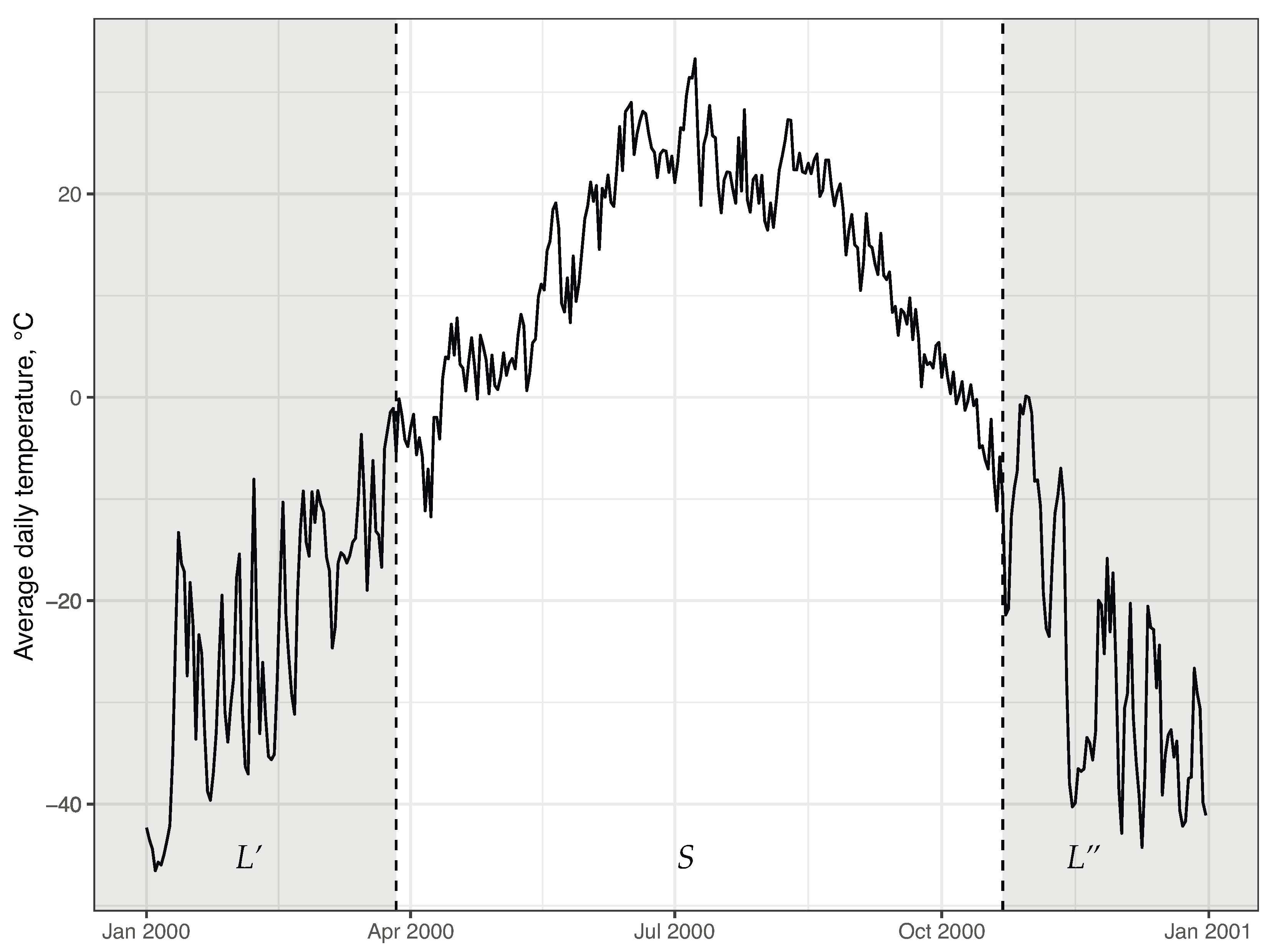
2.2. Calculation of Logging Season Duration

In Siberia, logging is only possible during the period when forest soils are frozen enough to use heavy logging machinery and usually spans the entirety of winter and part of the autumn and spring months (from late October to early April).

We used the following scheme of a typical year divided into different periods:

$$L^{{}^{\prime }}\to \omega \to S\to \omega \to L^{{}^{″}},$$

(1)

where $L^{{}^{\prime }}$—number of days since January 1 to the day when the temperature exceeds the threshold needed to start snow melting ($t^{+}$), ${\omega }^{+}$—window lag to let the snow cover become unsuitable for logging transportation, S—duration of non-logging period, ${\omega }^{-}$—window lag to let the ground freeze when the season is starting, $L^{{}^{″}}$—number of days since the season starts (temperature is below threshold of ground freezing $t^{-}$) to December 31 (Figure 2).

For this study, we supposed that the expectable logging season starts when the mean daily air temperature is $t^{-}=-5{}^{\circ }$C or below for three days (${\omega }^{-}=3$), and ends when the temperature is $t^{+}=0{}^{\circ }$C or above for three days as well (${\omega }^{+}=3$). The necessity of $\omega$ lag is explained with the fact that in forest sites, ground freezing and thawing processes are a lot slower than in the open-air territories due to less sunlight and litter presence. The three-day window lag appeared to be the best fit option for calculating the duration of the season. It is also possible to add to $\omega$ the time for construction of temporary roads but it may vary greatly depending on the distance to logging sites, relief characteristics, and snowpack height; therefore, we did not consider this period.

Severe Siberian climatic conditions limit logging activities in winters, as there are specific days when loggers are forced to stop their work in the open air because of the risk of frostbite (in Russian, these non-working days are called actirovannye dni). To obtain reliable and credible modeling results, we calculated and subtracted non-working cold days from the yearly duration of the season when loggers stop felling whilst cold and windy weather conditions occur, waiting for the end of the frost to proceed with harvesting operations. Thus, we estimated the period when logging activities could proceed. We calculated and subtracted non-working cold days from the yearly duration of the logging season to estimate the period when logging activities could proceed. The air temperature and wind speed thresholds at which operations in the open-air territories are temporarily suspended are usually stated by regional legislative legal acts and are different for each territory [40,41] (see

Table 2. Temperature (t, ${}^{\circ }$C) and wind speed (w, km/h) thresholds to declare actirovannye dni (non-working days) in Krasnoyarsk Krai and Irkutsk Oblast.

Krasnoyarsk		Irkutsk
$\mathit{t}$	$\mathit{w}$	$\mathit{t}$	$\mathit{w}$
$-40$	NA	40	NA
NA	22
$-35$	5	$-35$	3
$-25$	10
$-15$	15
$-5$	20

).

Though the cited documents are no longer valid, there are still no newly-established legal acts that define limitations on the working process during extreme weather conditions. Nevertheless, in real practice, these requirements are to be met, so we decided to follow the list of criteria provided by decrees and took into account a total number of non-working days.

As can be seen from Figure 3, the number of these days significantly differ across the observation period and meteorological stations. Only three stations experienced the average number of non-working days well above 0, while the rest, e.g., the southern stations, did not suffer significantly from extremely cold weather. In this regard, these non-working days were subtracted from the yearly duration of the logging season. Due to the recent climate change process, we supposed that eventually the number of non-working days will tend to decrease in long-run.

In terms of having enough bearing capacity of soils as a starting point for calculating the season bounds, the soil surface temperature seems more suitable as a measurement source; however, due to more gaps in observations, we preferred the dry-bulb thermometer air temperature. Our results showed a three-day delay until the forest ground froze enough to start the logging season. As a result, we calculated annual data on duration of timber harvesting season obtained from the meteorological stations of two Siberian regions.

Data preprocessing and further calculations were made using R software environment [34] with forecast [42,43], trend [44], imputeTS [45], and tseries [46] packages. Graphics and tables were designed with ggplot [47], corrplot [48], and xtable [49] packages.

2.3. Trend Presence Testing

To test the trend presence in time series of logging season duration, we used the well-known Mann–Kendall method [50,51]. This test was extensively employed for different kinds of climate change—studies on both environmental and economic effects [52,53,54,55,56].

Let $x_i$ be an element of time series X ($x_i\in X\forall i\in [1,n]$), then the S indicator is computed as

$$S=\sum _{i=1}^{n-1}\sum _{j=i+1}^{n}sgn(x_j-x_i),$$

where $sgn\left(\omega \right)$ denotes the conventional signum function, which is equal to 1 when $\omega >0$, it is $-1$, when $\omega <0$ and is zero when $\omega =0$.

Then the Kendall tau correlation coefficient is defined as

$$\tau ={\displaystyle \frac{S}{n(n-1)/2}}.$$

When n is high enough ($n>8$ according to [51]), the statistic S follows a normal distribution, with

$$z=sgn\left(S\right){\displaystyle \frac{\left|S\right|-1}{\sigma }}=sgn\left(S\right){\displaystyle \frac{18\left(\right|S|-1)}{n(n-1)(2n+5)-{\displaystyle \sum _{j=1}^p}{t}_j(t_j-1)(2t_j+5)}}.$$

A set of hypotheses for the test can be made as follows:

$$H_0:\mathrm{no}\mathrm{trend}\mathrm{exists},$$

$$H_1:\mathrm{a}\mathrm{trend}\mathrm{exists}.$$

If a trend exists at some significance level, its direction (decreasing or increasing) is determined based on the sign of the $\tau$ coefficient.

2.4. Modeling and Forecasting of Logging Season Duration

The methodology of forecasting of timber harvesting season duration dynamics is based on the well-known autoregressive-integrated-moving average modeling (ARIMA) framework suggested by G. Box and G. Jenkins in 1970 [57]. It is widely used in various disciplines, including some recent studies in forest economics [58,59,60].

The predictive side of the ARIMA $(p,d,q)$ model consists of two parts: the autoregressive term (AR) of order p and moving average term (MA) of order q. As the ARIMA model is only valid for stationary processes that keep constant distribution when shifted in time, the order d defines the necessary number of differences to be taken until the process is stationary. Under these conditions, the ARIMA model for $Y_t$ variable when $d=0$ is given as:

$$Y_t={\phi }_0+{\phi }_1{Y}_{t-1}+{\phi }_2{Y}_{t-2}+\dots +{\phi }_p{Y}_{t-p}+{\epsilon }_t+{\theta }_1{\epsilon }_{t-1}+{\theta }_2{\epsilon }_{t-2}+\dots +{\theta }_q{\epsilon }_{t-q}+e_t,$$

(2)

where ${\phi }_0$—constant (or intercept), ${\phi }_1,{\phi }_2,\dots ,{\phi }_p$ and ${\theta }_1,{\theta }_2,\dots ,{\theta }_q$—model parameters, $e_t$—error term.

In our study, we evaluated the time series ARIMA models using the algorithm described below for each station and then predicted the logging season duration.

• Box–Cox transformation (if needed). If the variance of a time series is not constant, the Box–Cox transformation makes the data approximate to a normal distribution according to the following rule:

  $$y\left(\lambda \right)=\left\{\begin{array}{cc}(y^{\lambda }-1)/\lambda ,\hfill & \mathrm{if}\lambda \ne 0;\hfill \\ ln\left(y\right),\hfill & \mathrm{otherwise}.\hfill \end{array}\right.$$

  (3)
  To select the value of $\lambda$ parameter, we used the technique proposed by V. M. Guerrero [61].
• Selection of the differencing degree. The most common tests for stationarity/non-stationarity are Augmented Dickey–Fuller (ADF) [62] and Kwiatkowski–Phillips–Schmidt–Shin (KPSS) [63]. For our research, we used the KPSS-test, which assumes a more easy-to-operate hypothesis of stationarity. When at some step the KPSS null-hypothesis of stationarity is not rejected, the d parameter of ARIMA model should be set to the current order of differencing.
• Fitting of p and q parameters. As there is no finite algorithm to calculate the numbers of AR and MA model components, the straightforward evaluation of all possible combinations was used. The maximum values of p and q were usually set to five. We used the Akaike information criterion (AIC) to select the best-fitted model. In our study, we employed Corrected Akaike information criterion (AICc), a modified AIC criterion for small samples. Its formula is given as:

  $$AICc=2(p+q+k+1)-2ln\left(\widehat{L}\right)+{\displaystyle \frac{2(p+q+k+1)(p+q+k+2)}{T-p-q-k-2}},$$

  (4)

  where k—flag of constant term presence ($k=1$ if ${\phi }_0\ne 0$, and $k=0$, otherwise) and $\widehat{L}$ is the maximum value of the likelihood function. A model with the lowest value of AICc should be selected as the best fit.
• Checking that residuals look like white noise. The Ljung–Box test was used to test whether there is no serial correlation in the residuals of the fitted model. If it is not the case, another model should be selected.

The forecast package implements the auto.arima function that allows for automating the procedure using the algorithm by R. Hyndman and Y. Khandakar [42]. In some cases, the algorithm suggests using a nonsense ARIMA(0,0,0) model, which represents a white noise process. Such models need to be manually replaced with the second-best fit according to the AICc.

3. Results and Discussion

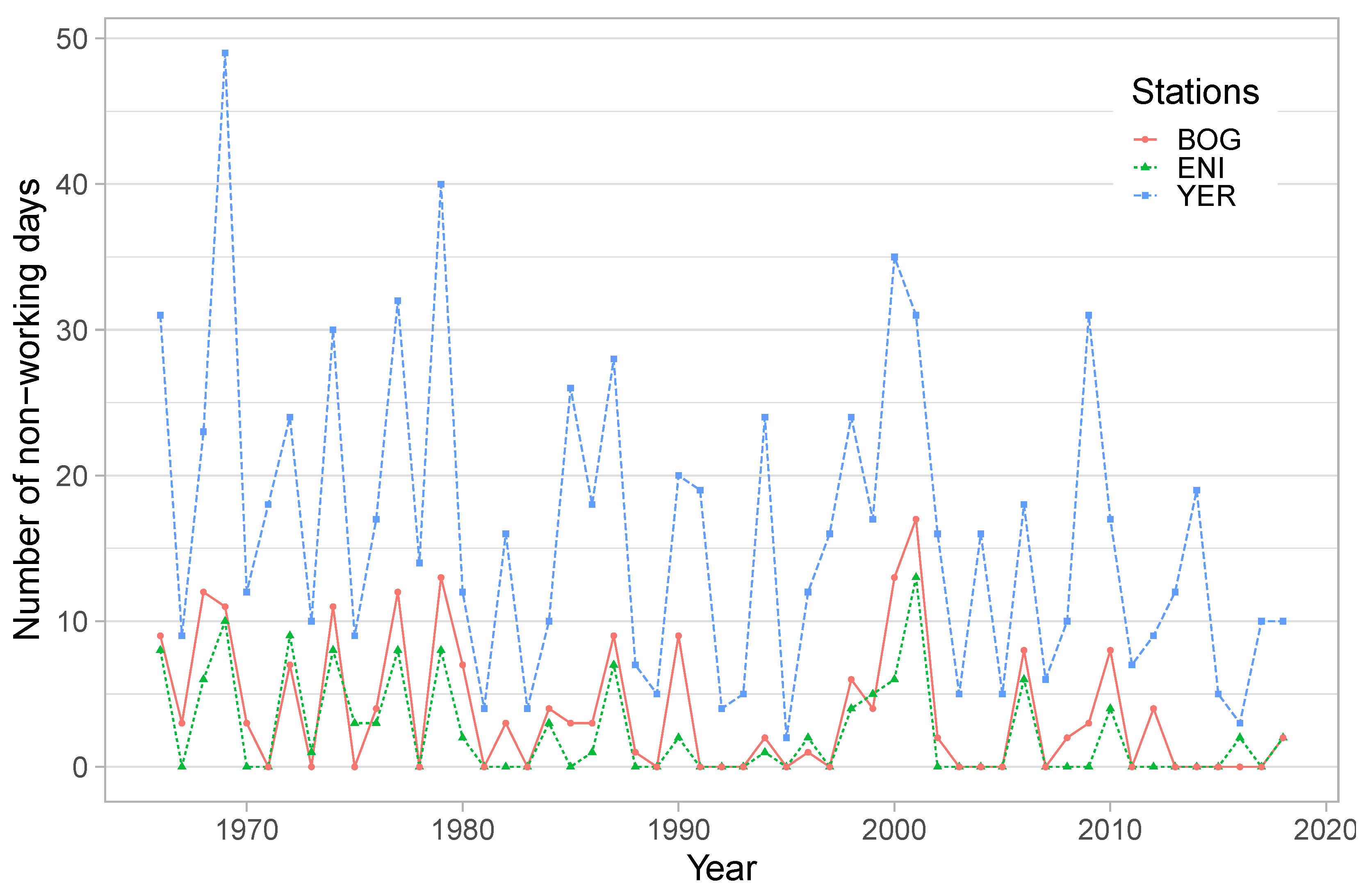
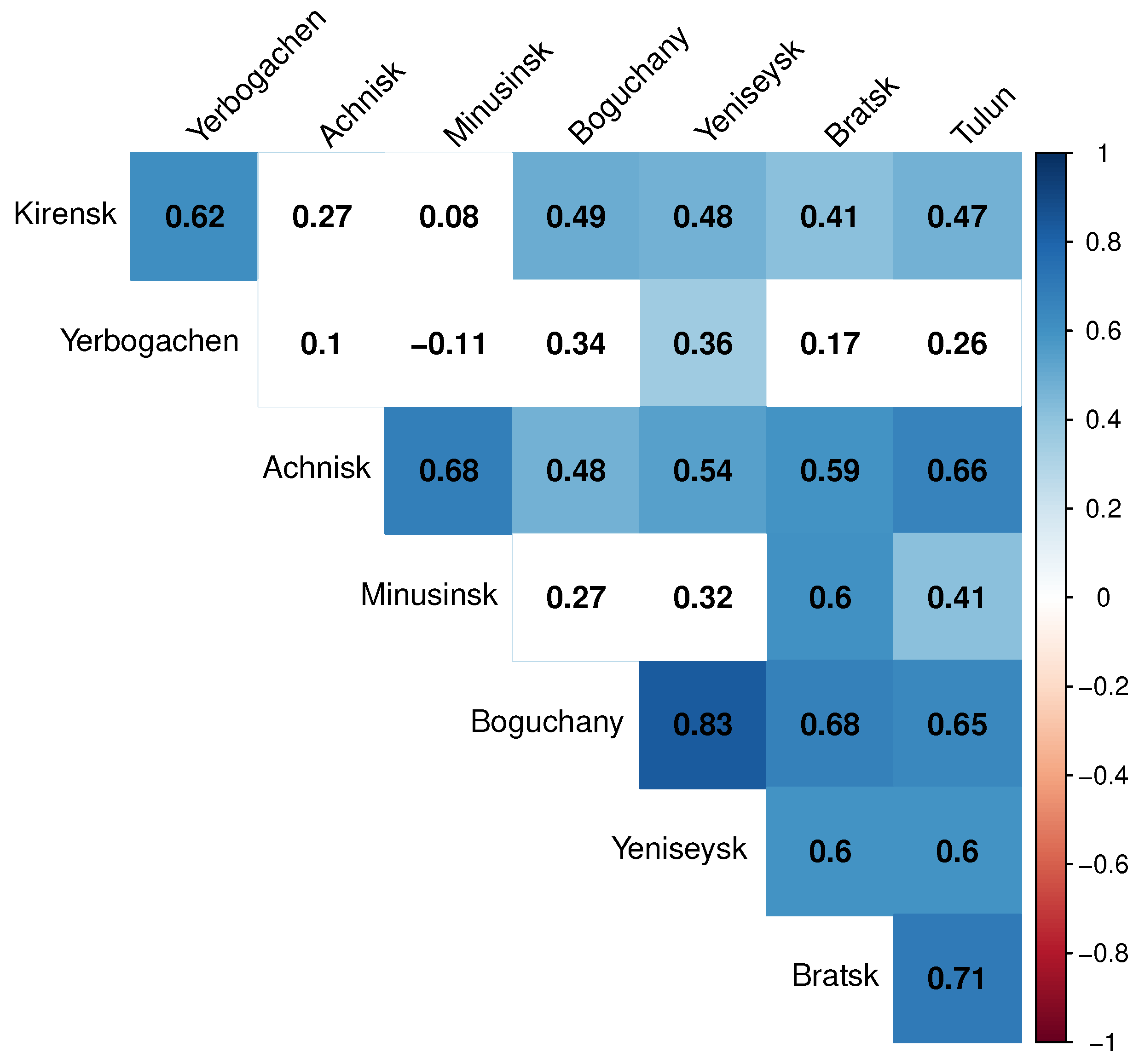
3.1. Logging Season Duration Shortening

The calculated logging season durations vary from station to station, largely depending on latitude: the southern Minusinsk provided in average 137.6 days of possible logging, but the northern Yerbogachen offered a month more (

Table 3. Basic descriptive statistics for calculated logging season durations and the Mann–Kendall test results for eight considered meteorological stations in Krasnoyarsk Krai and Irkutsk Oblast: 1966–2018.

	Station Name	Mean	S.D.	$\mathit{\tau }$	z	p-Value	Trend Characteristics
1	Acninsk	148.42	17.27	$-0.30$	$-3.15$	0.00	Decreasing trend
2	Boguchany	156.40	17.19	$-0.24$	$-2.53$	0.01	Decreasing trend
3	Bratsk	157.72	15.72	$-0.26$	$-2.74$	0.01	Decreasing trend
4	Kirensk	164.64	15.32	$-0.17$	$-1.77$	0.08	Decreasing trend
5	Minusinsk	137.58	14.37	$-0.20$	$-2.08$	0.04	Decreasing trend
6	Tulun	156.79	15.96	$-0.29$	$-3.07$	0.00	Decreasing trend
7	Yeniseysk	153.75	14.48	$-0.22$	$-2.34$	0.02	Decreasing trend
8	Yerbogachen	172.15	16.89	$-0.00$	$-0.01$	0.99	No trend

10% significance level is used for Mann–Kendall test interpretation.

).

There is a steady downward trend dynamics of the season duration for most meteorological stations. We supposed that non-working days calculated for these stations were expected to reduce and run out during the retrospective period 1966–2018. Krasnoyarsk Krai and Irkutsk Oblast are areas with harsh continental climate inherent to temperate latitudes with high-temperature volatility, nevertheless, for all stations except Yerbogachen, we observed decreasing trends in logging season duration at 10% significance level. The specificity of Yerbogachen is additionally explicit in the correlation matrix for the same logging season durations (Figure 4).

We identified a rather strong relationship between the logging season durations estimated for Yeniseysk and Boguchany ($r=0.83$). These meteorological stations are located in the watershed of major Siberian rivers (Yeniseysk is on the left bank of the Yenisey river, Boguchany is on the left bank of the Angara River). Though the sites are remote from each other, they are at the same latitude, hence, they experience similar alterations in local temperatures. Correlation between Achinsk and Minusinsk is less sharp ($r=0.68$), as they are located particularly at different latitudes to the southwest border of the region. Minusinsk is far away from Yeniseysk and Boguchany, which is reflected in the low corresponding correlation coefficients.

Irkutsk Oblast is bordered on the west by Krasnoyarsk Krai. Yerbogachen and Kirensk are geographically separated from the two other locations and situated in the northern part of the region, which points to a stronger linkage ($r=0.62$). In turn, the correlation of the logging season duration estimated between Bratsk and Tulun is high ($r=0.71$), which is explained by their location in the southwest part of the region with similar climatic conditions.

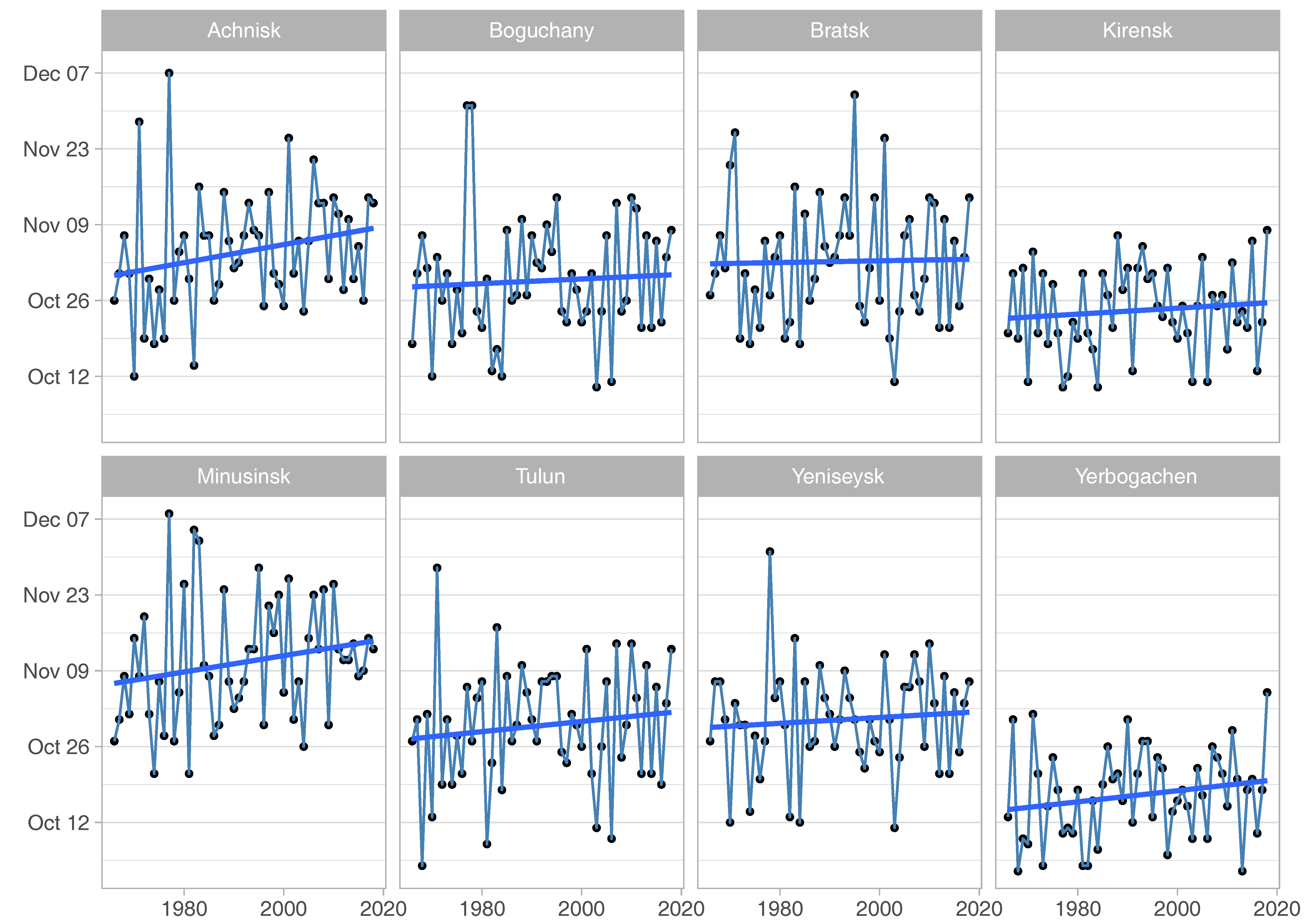
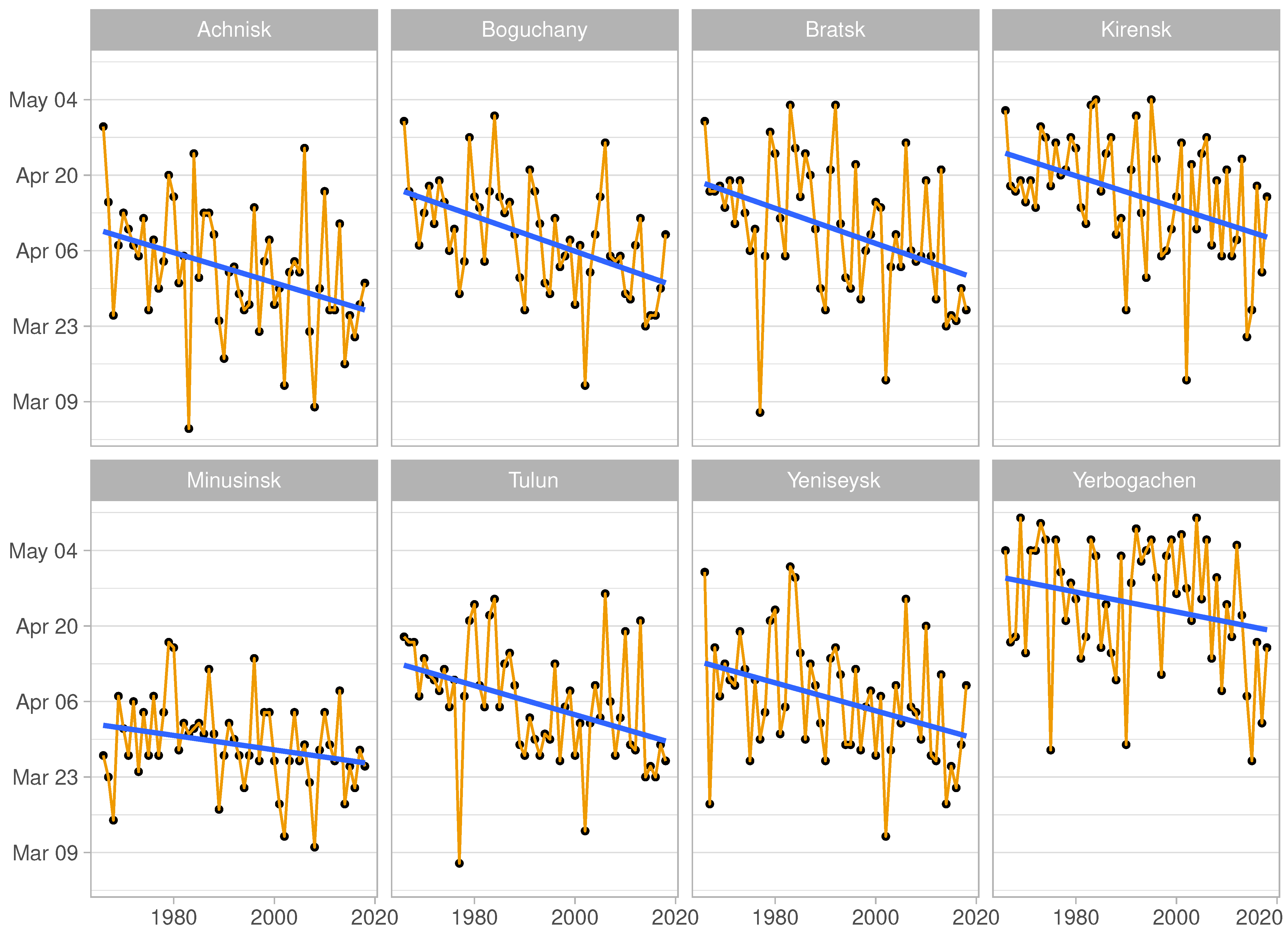
3.2. Tendencies of Expectable Season Start/End Boundaries

As the duration of logging seasons is shortened, it is important to study how this influences the season’s start and end boundaries. Figure 5 shows that the southern sites (Achinsk and Minusinsk) experienced an acute ten-day shift of the season start boundaries to later dates throughout the observation period, while logging season start boundaries remained almost constant for other sites.

Figure 6 depicts a much more pronounced shift of logging season end boundary. Though the average season end varied from the end of March to the end of May, all the stations witnessed at least a ten-day shift to earlier dates. That means the snow cover started to melt much earlier in the last decades.

The main conclusion is that the gradual reduction of the logging season duration has an uneven effect on the start and end boundaries of the season. Climate warming has practically no effect on the start date of the season in winter, but it significantly shifts the boundaries of the season end in spring. Although the considered stations are located in similar geographical conditions, the local climate differs significantly and affects the economic potential of logging activity.

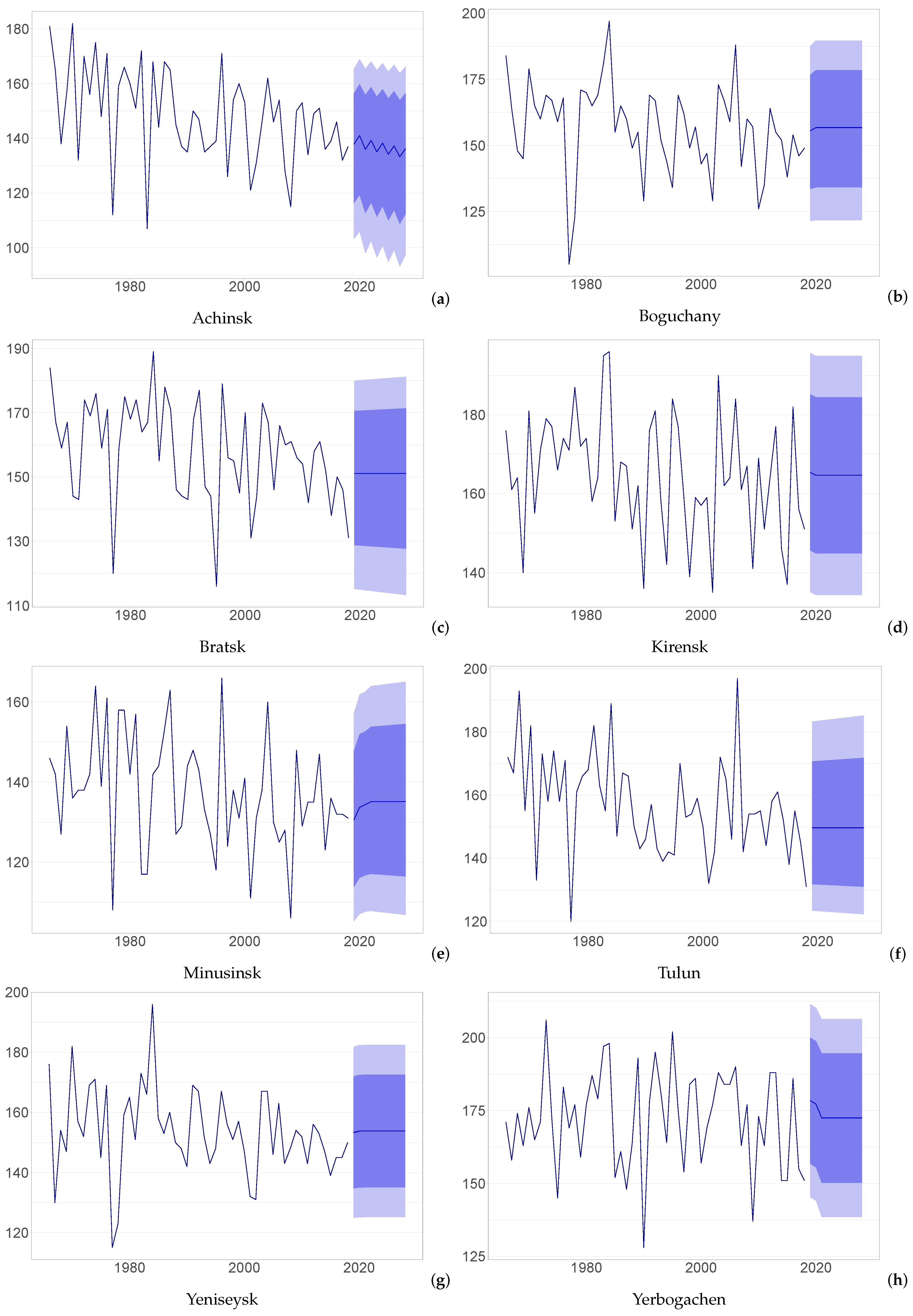
3.3. Logging Season Duration Modeling and Forecasting

We tested several model specifications for logging season duration and fitted the best ARIMA model for each of the meteorological stations (

Table 4. Estimates and performance characteristics for the best ARIMA models fitted.

	Station Name	$(\mathit{p},\mathit{d},\mathit{q})$	Mean/Drift	${\mathit{\phi }}_1$	${\mathit{\theta }}_1$	${\mathit{\theta }}_2$	${\mathit{\theta }}_3$	${\mathit{\theta }}_4$	AICc
1	Achinsk	$(1,1,4)$	$-64.75$	$-0.99$	$-0.29$	$-1.22$	$0.26$	$0.36$	$959.27$
			$\left(18.12\right)$	$\left(0.03\right)$	$\left(0.14\right)$	$\left(0.15\right)$	$\left(0.15\right)$	$\left(0.17\right)$
2	Boguchany	$(0,0,1)$	$513.87$		$0.25$				$606.45$
			$\left(11.87\right)$		$\left(0.15\right)$
3	Bratsk	$(0,1,1)$		$-0.90$					$963.56$
				$\left(0.06\right)$
4	Kirensk	$(0,0,1)$	$164.64$		$-0.05$				$445.05$
			$\left(1.98\right)$		$\left(0.15\right)$
5	Minusinsk	$(0,1,4)$			$-1.32$	$0.27$	$-0.17$	$0.34$	$293.81$
					$\left(0.16\right)$	$\left(0.28\right)$	$\left(0.27\right)$	$\left(0.14\right)$
6	Tulun	$(0,1,1)$		$-0.89$					$-217.51$
				$\left(0.07\right)$
7	Yeniseysk	$(1,0,0)$	$153.81$	$0.13$					$438.38$
			$\left(2.24\right)$	$\left(0.14\right)$
8	Yerbogachen	$(0,0,2)$	$172.44$		$-0.05$	$-0.23$			$455.74$
			$\left(1.66\right)$		$\left(0.14\right)$	$\left(0.17\right)$

Standard errors are in parentheses under the corresponding parameter estimates.

). As the time series of logging season duration is measured on a yearly basis and are quite short in terms of time-series modeling (1966–2018), the most part of the obtained models captures short-run dynamics with one or two lags. The models for Achinsk and Minusinsk include up to four lags in the MA component, thus reflecting a more prolonged impact of previous years dynamics of logging season duration.

The most common specification of ARIMA models that are employed in our analysis was the moving average model. In the statistical and econometrical analysis, ARIMA (0,1,1) is referred to as simple exponential smoothing, i.e., non-stationary time series model with first-order differencing and MA(1) term.

Except for Boguchany and Yeniseisk, ARIMA model coefficients are negative for the rest of the stations, which indicates the fading trends in the values of time series. If the trend continues in the future, the dispersion of the indicator will narrow and the time series levels will decrease. Certain individual positive coefficients (e.g., ${\theta }_3=0.26,$${\theta }_4=0.36$ for Achinsk and ${\theta }_2=0.27$, ${\theta }_4=0.34$) do not change this conclusion, as the sum of coefficients, which accounts for cumulative effect, is negative in both cases.

The check of residuals for all the models showed that there is no serial correlation and no evidence to reject the hypothesis that the distribution of residuals does not fit the normal law. We omit the corresponding graphs and Ljung–Box diagnostic test statistics, as they do not contain any information that could contribute to the following analysis.

In addition to the task of analyzing retrospective trends in logging season duration, ARIMA models can be conveniently used to produce forecasts. A 10-year forecasted point of logging season durations for all the stations were calculated along with the corresponding confidence intervals (Figure 7). Historical data are depicted as dark blue lines, 95% and 80% confidence intervals around the point forecasts for the next 10 years are drawn as green bands of different opacity. Observed values of logging season durations have wide amplitude fluctuations and differ dramatically through the overall baseline period that points at high variability in season length. We defined outliers of the lowest values in time series data assuming that some shorter seasons can be explained by late winter onsets and earlier thawing processes. On both Yeniseysk and Boguchany, the shortest duration of timber harvesting season reached 130 days per year in 1978. Lower values of 107 days in 1983 and 106 days in 2008 were identified on Achinsk and Minusinsk. When we considered the Bratsk and Tulun meteorological stations, duration of the season dropped to 123 in 1995 and 127 days per year in 1977 correspondingly, but it did not fall below 137 days as for Kirensk and Yerbogachen.

All the forecasts contain non-positive tendencies of logging season duration. For Achinsk there is an evident negative trend, which predicts that the logging season will decrease from $148.4\pm 17.3$ days during the historical sample (1966–2018) to $136.2\pm 30$ days in 2028. In Bratsk, the decrease will be from $157.7\pm 15.7$ to $151.1\pm 29.9$, in Tulun, from $156.8\pm 15.9$ to $149.6\pm 35.5$ days, in Minusinsk, from $137.6\pm 14.4$ to $135.1\pm 29.9$ days. As for other stations, the lack of data does not allow us to produce more lagged ARIMA models, the forecast for them does not show any significant reduction of future values of logging season durations. However, the observed trends in reduced season duration for all stations, as well as high correlations between indicators for different stations, suggest that a gradual reduction in logging season duration, proportional to the results obtained for Achinsk, will be observed in the entire observed area.

Although all these areas are under a temperate-climate zone with a harsh continental climate, there is a set of microclimate characteristics specific to the particular local area and depending on proximity to major watersheds as well as topography that lead to different forecast findings across the stations. For instance, a one-day reduction in season duration in Minusinsk implies no significant changes in temperature regimes for this area that can be explained by the specific geography of this station in terms of relief characteristics. Minusinsk is in the center of the same name. Hollow were driven by anticyclonic weather conditions cold air flows down the slopes to the hollow’s bottom and stays there during winters thus forming a stable local climate that is poorly affected by warming processes occurring at higher elevations [64].

Calculated data on Yerbogachen as the northernmost meteorological station pointed at a larger number of non-working days with the most prolong unfavorable weather conditions period (non-working days) of 56 days in 1969. We assumed that due to the rising air temperatures the season should start later but ends earlier over time. Meanwhile, the number of cold windy days with high frostbite risk tends to diminish so ARIMA modeling produces duration of the season as generally permanent and stable, i.e., without any dynamics in the short run term of 20 years. However, non-working days will eventually run out supporting the idea of gradual shortening timber harvesting season for this meteorological station.

4. Conclusions

Climate change has become a major topic of study throughout many scientific domains, since there is a consensus that this problem is one of the main global challenges for the human civilization of future decades. Special attention is paid to the negative consequences of climate change for both environment and economy. Global climate change is one of the most important issues for forest economics, since it may impact the resource base of the logging industry in different ways depending on specific climatic, geographic, and economic conditions, and these questions need to be answered at the regional scale.

In the Siberian regions, the major reason for poor accessibility to forest areas is the presence of wet forest soils, which prevents logging machinery from moving towards felling sites in frost-free time. Hence, forest logging activities are implemented during the period with a permanent snow cover and stable sub-zero temperatures when forest grounds freeze enough to bear heavy machinery. In this study, we identified this period as timber harvesting season. Taking into account the recent global climate change process, the duration of timber harvesting season is supposed to get shorter as time passes.

We introduced a concept for calculating the duration of the logging season for the largest Siberian regions, taking into account the economic and climatic peculiarities of doing business in these territories. The climatic data from Roshydromet were used to calculate the duration of logging season for eight representative stations in Krasnoyarsk Krai (Yeniseysk, Boguchany, Achinsk, Minusinsk) and Irkutsk Oblast (Bratsk, Kirensk, Tulun, Yerbogachen) for the period 1966–2018.

The main conclusions of our analysis are summarized below.

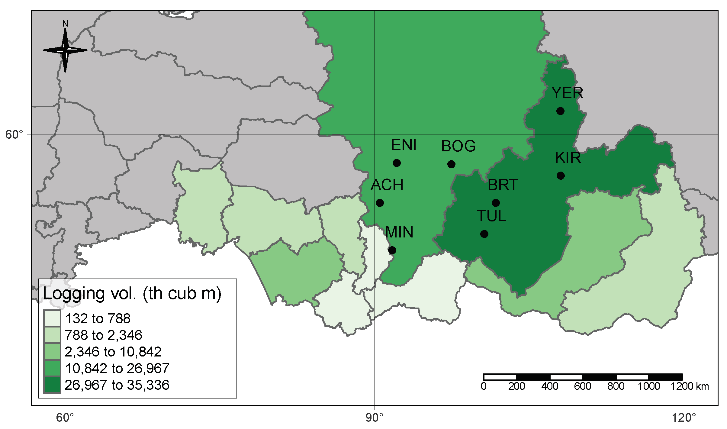
• There is strong evidence of logging season duration shortening during the retrospective period of 1966–2018 for almost all considered stations. Although the considered stations are located in similar natural conditions, the local climate varies significantly and affects the economic potential of logging activity.
• The gradual reduction of logging season durations has an uneven effect on the start and end boundaries of the season. Climate warming has almost no effect on the start date of the season in winter, but it significantly shifts the boundaries of the season end in spring.
• Despite some limitations of ARIMA modeling framework forecasting performance caused by the lack of prolonged-time series of temperature and wind speed available for calculating the logging season durations, a set of ARIMA models of acceptable quality was elaborated. These forecasting models show that in the nearest future, the trends of gradual shortening of logging season duration will hold for the most part of stations. The most pronounced effect is observed for Achinsk station, where, according to our calculations the logging season will decrease from $148.4\pm 17.3$ days during the historical sample (1966–2018) to $136.2\pm 30$ days in 2028.
• In our opinion, the identified downward trends in the duration of the potential logging season in the largest Siberian logging regions are a direct consequence of the global climate change observed during the period on which the database used was based.
• From an economic perspective, shorter duration of logging season means fewer wood stocks available for cutting that would make companies unable to comply with their logging plans and lead them to suffer losses in the future. In this regard, logging companies will have to adapt to these changes by redefining their economic strategies in terms of intensifying timber harvesting operations.
• The approach we used in this study might be applied to the prediction of establishment and then the loss of ice roads to access remote mines and communities in circumpolar areas.

References

1. Bukvareva, E.N.; Grunewald, K.; Bobylev, S.N.; Zamolodchikov, D.G.; Zimenko, A.V.; Bastian, O. The current state of knowledge of ecosystems and ecosystem services in Russia: A status report. Ambio 2015, 44, 491–507. [Google Scholar] [CrossRef] [Green Version]
2. IPCC. Climate Change 2014: Synthesis Report. Contribution of Working Groups I, II and III to the Fifth Assessment Report of the Intergovernmental Panel on Climate Change; Cambridge University Press: Cambridge, UK; New York, NY, USA, 2013. [Google Scholar] [CrossRef] [Green Version]
3. Tol, R.S.J. The Economic Effects of Climate Change. J. Econ. Perspect. 2009, 23, 29–51. [Google Scholar] [CrossRef] [Green Version]
4. Bosello, F.; Roson, R.; Tol, R.S. Economy-wide estimates of the implications of climate change: Human health. Ecol. Econ. 2006, 58, 579–591. [Google Scholar] [CrossRef] [Green Version]
5. Dell, M.; Jones, B.F.; Olken, B.A. Climate Change and Economic Growth: Evidence from the Last Half Century; Working Paper 14132; National Bureau of Economic Research: Cambridge, MA, USA, 2008. [Google Scholar]
6. Maddison, D. The amenity value of the climate: The household production function approach. Resour. Energy Econ. 2003, 25, 155–175. [Google Scholar] [CrossRef]
7. Labriet, M.; Joshi, S.R.; Vielle, M.; Holden, P.B.; Edwards, N.R.; Kanudia, A.; Loulou, R.; Babonneau, F. Worldwide impacts of climate change on energy for heating and cooling. Mitig. Adapt. Strateg. Glob. Chang. 2015, 7, 1111–1136. [Google Scholar] [CrossRef] [Green Version]
8. Rehdanz, K.; Maddison, D. Climate and happiness. Ecol. Econ. 2005, 52, 111–125. [Google Scholar] [CrossRef]
9. Boisvenue, C.; Running, S.W. Impacts of climate change on natural forest productivity–evidence since the middle of the 20th century. Glob. Chang. Biol. 2006, 12, 862–882. [Google Scholar] [CrossRef]
10. Lutz, D.A.; Shugart, H.H.; White, M.A. Sensitivity of Russian forest timber harvest and carbon storage to temperature increase. Forestry 2013, 86, 283–293. [Google Scholar] [CrossRef] [Green Version]
11. Garcia-Gonzalo, J.; Peltola, H.; Briceño-Elizondo, E.; Kellomäki, S. Effects of climate change and management on timber yield in boreal forests, with economic implications: A case study. Ecol. Modell. 2007, 209, 220–234. [Google Scholar] [CrossRef]
12. Kirilenko, A.P.; Sedjo, R.A. Climate change impacts on forestry. Proc. Natl. Acad. Sci. USA 2007, 104, 19697–19702. [Google Scholar] [CrossRef] [Green Version]
13. Tian, X.; Sohngen, B.; Kim, J.B.; Ohrel, S.; Cole, J. Global climate change impacts on forests and markets. Environ. Res. Lett. 2016, 11, 035011. [Google Scholar] [CrossRef]
14. Brecka, A.F.J.; Shahi, C.; Chen, H.Y.H. Climate change impacts on boreal forest timber supply. For. Policy Econ. 2018, 11–21. [Google Scholar] [CrossRef]
15. Goltsev, V.; Lopatin, E. The impact of climate change on the technical accessibility of forests in the Tikhvin District of the Leningrad Region of Russia. Int. J. For. Eng. 2013, 24, 148–160. [Google Scholar] [CrossRef]
16. Saad, C.; Boulanger, Y.; Beaudet, M.; Gachon, P.; Ruel, J.C.; Gauthier, S. Potential impact of climate change on the risk of windthrow in eastern Canada’s forests. Clim. Chang. 2017, 487–501. [Google Scholar] [CrossRef]
17. Ivantsova, E.D.; Pyzhev, A.I.; Zander, E.V. Economic Consequences of Insect Pests Outbreaks in Boreal Forests: A Literature Review. J. Sib. Fed. Univ. Humanit. Soc. Sci. 2019, 627–642. [Google Scholar] [CrossRef] [Green Version]
18. Shvidenko, A.Z.; Schepaschenko, D.G. Climate change and wildfires in Russia. Contemp. Probl. Ecol. 2013, 7, 683–692. [Google Scholar] [CrossRef]
19. Kharuk, V.I.; Im, S.T.; Petrov, I.A.; Golyukov, A.S.; Ranson, K.J.; Yagunov, M.N. Climate-induced mortality of Siberian pine and fir in the Lake Baikal Watershed, Siberia. For. Ecol. Manag. 2017, 384, 191–199. [Google Scholar] [CrossRef]
20. Tchebakova, N.M.; Parfenova, E.I.; Korets, M.A.; Conard, S.G. Potential change in forest types and stand heights in central Siberia in a warming climate. Environ. Res. Lett. 2000, 11, 035016. [Google Scholar] [CrossRef] [Green Version]
21. Hanewinkel, M.; Cullmann, D.A.; Schelhaas, M.J.; Nabuurs, G.J.; Zimmermann, N.E. Climate change may cause severe loss in the economic value of European forest land. Nat. Clim. Chang. 2000, 203–207. [Google Scholar] [CrossRef]
22. Fei, S.; Desprez, J.M.; Potter, K.M.; Jo, I.; Knott, J.A.; Oswalt, C.M. Divergence of species responses to climate change. Sci. Adv. 2017, 3, e1603055. [Google Scholar] [CrossRef] [Green Version]
23. Drobyshev, I.; Gewehr, S.; Berninger, F.; Bergeron, Y. Species specific growth responses of black spruce and trembling aspen may enhance resilience of boreal forest to climate change. J. Ecol. 2013, 1, 231–242. [Google Scholar] [CrossRef] [Green Version]
24. Johnstone, J.F.; Hollingsworth, T.N.; Chapin, F.S.; Mack, M.C. Changes in fire regime break the legacy lock on successional trajectories in Alaskan boreal forest. Glob. Chang. Biol. 2013, 4, 1281–1295. [Google Scholar] [CrossRef]
25. Rittenhouse, C.D.; Rissman, A.R. Changes in winter conditions impact forest management in north temperate forests. J. Environ. Manag. 2015, 157–167. [Google Scholar] [CrossRef] [PubMed]
26. Hellmann, L.; Tegel, W.; Kirdyanov, A.V.; Eggertsson, Ó.; Esper, J.; Agafonov, L.; Nikolaev, A.N.; Knorre, A.A.; Myglan, V.S.; Sidorova, O.C.; et al. Timber Logging in Central Siberia is the Main Source for Recent Arctic Driftwood. Arct. Antarct. Alp. Res. 2015, 47, 449–460. [Google Scholar] [CrossRef] [Green Version]
27. Kuloglu, T.Z.; Lieffers, V.J.; Anderson, A.E. Impact of Shortened Winter Road Access on Costs of Forest Operations. Forests 2019, 10, 447. [Google Scholar] [CrossRef] [Green Version]
28. FAO. Global Forest Resources Assessment 2015. Country Report. Russian Federation. Available online: http://www.fao.org/3/a-az316e.pdf (accessed on 27 April 2020).
29. Rosstat. Unified Interdepartmental Information and Statistical System (EMISS). Harvested Wood Volume. Available online: https://fedstat.ru/indicator/37848 (accessed on 27 August 2019).
30. LUKE. Finnish Forest Statistics. Available online: https://stat.luke.fi/sites/default/files/suomen_metsatilastot_2019_verkko2.pdf (accessed on 27 April 2020).
31. Mokhirev, A.P.; Medvedev, S.O.; Smolina, O.N. Factors influencing the accessibility of timber transport roads. For. Eng. J. 2019, 103–113. [Google Scholar] [CrossRef]
32. Pyzhev, A.I. Global climate change and logging volumes in Siberian regions from 1946 to 1992. Terra Econ. 2020, 18, 140–153. [Google Scholar] [CrossRef]
33. Gordeev, R.V.; Pyzhev, A.I. Analysis of the Global Competitiveness of the Russian Timber Industry. ECO 2015, 109–130. [Google Scholar] [CrossRef]
34. R Core Team. R: A Language and Environment for Statistical Computing. Available online: https://www.R-project.org/ (accessed on 7 August 2019).
35. Pebesma, E. Simple Features for R: Standardized Support for Spatial Vector Data. R J. 2018, 10, 439–446. [Google Scholar] [CrossRef] [Green Version]
36. Tennekes, M. Tmap: Thematic Maps in R. J. Stat. Softw. 2018, 84, 1–39. [Google Scholar] [CrossRef] [Green Version]
37. South, A. Rnaturalearth: World Map Data from Natural Earth. R Package Version 0.1.0. Available online: https://CRAN.R-project.org/package=rnaturalearth (accessed on 8 December 2019).
38. Bulygina, O.; Veselov, V.; Razuvaev, V.; Aleksandrova, T. Description of Hourly Data Set of Meteorological Parameters Obtained at Russian Stations. Available online: http://meteo.ru/english/climate/descrip12.htm (accessed on 5 December 2019).
39. Veselov, V.; Pribylskaya, I. AISORI Specialized Technology. Available online: http://aisori.meteo.ru/ClimateR (accessed on 5 December 2019).
40. Administration of Krasnoyarsk Krai. The Decree Dated November 12, 2001 under no. 786-P on Operating Conditions during the Cold Season; Administration of Krasnoyarsk Krai: Krasnoyarsk Krai, Russia, 2001; Available online: http://docs.cntd.ru/document/985003848 (accessed on 12 May 2019).
41. Administration of Irkutsk Oblast. The Decree Dated September 26, 2001 under no. 33/201-pg on the Temperature Limits When Operating Outdoors and in Enclosed Unheated Rooms during the Cold Season; Administration of Irkutsk Oblast: Irkutsk, Russia, 2001; Available online: http://docs.cntd.ru/document/469412568 (accessed on 12 May 2019).
42. Hyndman, R.J.; Khandakar, Y. Automatic time series forecasting: The forecast package for R. J. Stat. Softw. 2008, 26, 1–22. [Google Scholar] [CrossRef]
43. Hyndman, R.; Athanasopoulos, G.; Bergmeir, C.; Caceres, G.; Chhay, L.; O’Hara-Wild, M.; Petropoulos, F.; Razbash, S.; Wang, E.; Yasmeen, F. Forecast: Forecasting Functions for Time Series and Linear Models. R Package Version 8.12. Available online: http://pkg.robjhyndman.com/forecast (accessed on 4 May 2020).
44. Pohlert, T. Trend: Non-Parametric Trend Tests and Change-Point Detection. R Package Version 1.1.2. Available online: https://CRAN.R-project.org/package=trend (accessed on 8 May 2020).
45. Moritz, S.; Bartz-Beielstein, T. imputeTS: Time Series Missing Value Imputation in R. R J. 2017, 9, 207–218. [Google Scholar] [CrossRef] [Green Version]
46. Trapletti, A.; Hornik, K. Tseries: Time Series Analysis and Computational Finance. R Package Version 0.10-47. Available online: https://CRAN.R-project.org/package=tseries (accessed on 8 May 2020).
47. Wickham, H. Ggplot2: Elegant Graphics for Data Analysis; Springer: New York, NY, USA, 2016. [Google Scholar]
48. Wei, T.; Simko, V. R Package “Corrplot”: Visualization of a Correlation Matrix. (Version 0.84). Available online: https://github.com/taiyun/corrplot (accessed on 8 May 2020).
49. Dahl, D.B.; Scott, D.; Roosen, C.; Magnusson, A.; Swinton, J. Xtable: Export Tables to LaTeX or HTML, R package version 1.8-4; 2019. Available online: https://CRAN.R-project.org/package=xtable (accessed on 12 May 2020).
50. Mann, H.B. Nonparametric Tests Against Trend. Econom. J. Econom. Soc. 1945, 13, 245–259. [Google Scholar] [CrossRef]
51. Kendall, M.G. Multivariate Analysis; Griffin: London, UK, 1975. [Google Scholar]
52. Chen, W.J. Is the Green Solow Model Valid for CO2 Emissions in the European Union? Environ. Resour. Econ. 2017, 67, 23–45. [Google Scholar] [CrossRef]
53. Hamed, K.H.; Ramachandra Rao, A. A modified Mann-Kendall trend test for autocorrelated data. J. Hydrol. 1998, 204, 182–196. [Google Scholar] [CrossRef]
54. Škvareninová, J.; Tuhárska, M.; Škvarenina, J.; Babálová, D.; Slobodníková, L.; Slobodník, B.; Středová, H.; Minďaš, J. Effects of light pollution on tree phenology in the urban environment. Morav. Geogr. Rep. 2017, 25, 282–290. [Google Scholar] [CrossRef] [Green Version]
55. Yue, S.; Wang, C. The Mann-Kendall Test Modified by Effective Sample Size to Detect Trend in Serially Correlated Hydrological Series. Water Resour. Manag. 2004, 18, 201–218. [Google Scholar] [CrossRef]
56. Vido, J.; Tadesse, T.; Šustek, Z.; Kandrík, R.; Hanzelová, M.; Jaroslav, S.; Škvareninová, J.; Hayes, M. Drought Occurrence in Central European Mountainous Region (Tatra National Park, Slovakia) within the Period 1961–2010. Adv. Meteorol. 2015, 2015. [Google Scholar] [CrossRef] [Green Version]
57. Box, G.E.P.; Jenkins, G.M. Time Series Analysis: Forecasting and Control; Holden-Day: San Francisco, CA, USA, 1970; p. 553. [Google Scholar]
58. Lin, M.; Zhang, Z.; Cao, Y. Forecasting Supply and Demand of the Wooden Furniture Industry in China. For. Prod. J. 2019, 69, 228–238. [Google Scholar] [CrossRef]
59. Michinaka, T.; Kuboyama, H.; Tamura, K.; Oka, H.; Yamamoto, N. Forecasting Monthly Prices of Japanese Logs. Forests 2016, 7, 94. [Google Scholar] [CrossRef] [Green Version]
60. Buratto, D.; Junior, R.T.; Silva, J.; Frega, J.; Wiecheteck, M.; Silva, C. Use of Artificial Neural Networks and ARIMA to Forecasting Consumption Sawnwood of Pinus sp. in Brazil. Int. For. Rev. 2019, 21, 51–61. [Google Scholar] [CrossRef]
61. Guerrero, V.M. Time-series analysis supported by power transformations. J. Forecast. 1993, 12, 37–48. [Google Scholar] [CrossRef]
62. Said, S.E.; Dickey, D.A. Testing for unit roots in autoregressive-moving average models of unknown order. Biometrika 1984, 71, 599–607. [Google Scholar] [CrossRef]
63. Kwiatkowski, D.; Phillips, P.C.; Schmidt, P.; Shin, Y. Testing the null hypothesis of stationarity against the alternative of a unit root: How sure are we that economic time series have a unit root? J. Econom. 1992, 54, 159–178. [Google Scholar] [CrossRef]
64. Sukhova, M.G. Climate and Recreational-Climatic Resources of Altai-Sayan Mountainous Region Landscapes. Probl. Contemp. Sci. Pract. Vernadsky Univ. 2009, 2, 82–84. [Google Scholar]
Figure 1. Study sites and spatial distribution of logging volumes by Siberian regions in 2018 (thousands cubic meters). Note: developed by authors using R and sf, tmap, and rnaturalearth packages [34,35,36,37]. Data source: Rosstat [29].
Forests 11 00756 g001
Figure 2. Diagram of the temperature and calculated logging season (shapes L and L ) and non-logging period (shape S) for the sample Boguchany station (World Meteorological Organization (WMO) index = 29,282) in 2000.
Forests 11 00756 g002
Figure 3. Dynamics of within-year non-working days number for Boguchany (BOG), Yeniseysk (ENI), and Yerbogachen(YER): 1966–2018. Note: for other stations, the average number of non-working days does not significantly differ from 0.
Forests 11 00756 g003
Figure 4. Pearson correlations between expectable durations of logging seasons by meteorological stations of Krasnoyarsk Krai and Irkutsk Oblast: 1966–2018.
Forests 11 00756 g004
Figure 5. Annual shifts of season start boundary.
Forests 11 00756 g005
Figure 6. Annual shifts of season end boundary.
Forests 11 00756 g006
Figure 7. Point forecasts and forecast intervals at 80% and 95% levels of the expected duration of logging season by stations predicted with autoregressive-integrated-moving average modeling (ARIMA) models.
Forests 11 00756 g007