Landscape Preference for Trees Outside Forests along an Urban–Rural–Natural Gradient

Abstract

In densely populated areas, essential sources of ecosystem services are represented by green infrastructure, which includes trees outside forests (TOF) that, regardless of their cover extension, are found on agricultural or urban land. This research aims to assess landscape preference for TOF along an urban-rural-natural gradient in relation to different levels of landscape heterogeneity. Analyses are based on the integration of a visual choice experiment (360 respondents) with a GIS-based landscape analysis at regional scale in a Mediterranean region in Central Italy. Main findings revealed that correlation between landscape preference and heterogeneity varies along the urban–rural–natural gradient and on the basis of the spatial configuration of the surrounding landscape. The additional value of TOF to landscape preference is closely and positively linked to the degree of landscape anthropization. Conversely, TOF contribution to landscape preference resulted negative in natural landscapes where they can be perceived as a disturbance of the wilderness. Considering the influence that landscape preference plays on cultural ecosystem services provisioning and, in turn, on decision making processes, our results can support landscape policy and planning in fostering or hampering TOF diffusion depending on the different territorial contexts. These findings endorse the importance of multi-functional approaches in future-oriented strategies, which should mediate between the human preference for TOF, their ecological role and the provision of other services.

1. Introduction

Trees outside forests (TOF) generate many benefits from environmental, social and economic perspectives, hence they have received much attention in recent years. Trees outside forests are defined as all trees and shrubs that cannot be included in the “forests” nor in the “other wooded lands” categories of the FAO forest classification. Therefore, all trees growing in agricultural, urban or natural landscapes covering less than 0.5 ha and less than 20 m in width, are considered as TOF [1]. They include several tree formations, from single trees to systematically managed trees in agroforestry systems [2]. In several land mosaics worldwide, people use them for many purposes, including food provisioning, income, and biological diversity [1], or indirectly benefit from their role in landscape connectivity [3].

A striking case is the Mediterranean region, where most natural landscapes have been replaced by cultural landscapes deriving from the reorganization of land use and cover in order to adapt to changing social needs [4]. The cultural Mediterranean landscape is, therefore, one of the most typical settings for TOF because it is shaped by a complex heterogeneous mosaic of tree formations intermixed with agricultural land and settlements. For example, in Italy, TOF substantially contribute to landscape diversification and this role has been emphasized by recent land-use change dynamics [5]. Moreover, among the TOF forming the cornerstone of the ecological network of one the most intensively cultivated and urbanized regions in Europe, the Po Plain, there are hedgerows [6], and small woodland patches [7].

The presence of TOF contributes to the landscape view, from several perspectives. It is therefore challenging and important for policy makers trying to assess whether they are drivers of landscape preference. Since TOF generally grow in the human-nature interface, as in the urban fringe, they are directly exposed to human pressures [5] and human-induced landscape dynamics [8]. Nevertheless, an incomplete understanding of potential TOF-related services still often precludes their inclusion in global and national forest resource management and monitoring systems [9]. Consequently, the effective implementation of dedicated conservation and improvement actions often remains an unresolved issue [9].

One way to study landscape preference is to perform a visual choice experiment where respondents are asked to rank different pictures. This is commonly done using photographs, modified by a computer, controlling their content and hence the evaluation by a respondent under different scenarios [10]. This perception-based experiment has proved to be able to capture landscape preferences and offer a high level of reliability [11]. Moreover, removing or replacing objects through combining a geographic information system (GIS) and photographs makes it possible to infer which are the drivers of landscape preference [12]. Crossing urban and peri-urban boundaries, landscape preference for TOF patches could be associated to their key role on landscape structure [5], often being the main antagonists to landscape homogenization and scenic monotony. Landscape metrics, such as fragmentation and shape, are known to be statistically significantly correlated with preference, even more so than the characteristics of respondents [10]. Many integrated studies have been conducted through the analysis of correlations between landscape preference and landscape metrics [13,14,15,16,17,18].

Preference for landscape features has been commonly assessed in a single type of landscape, either natural, semi-natural, agricultural or urban [19]. However, landscape-related characteristics in which they are set may also play a fundamental role in modifying the preference for single features. In particular, along an urban–rural–natural gradient of landscape types, the level of human influence will change, and this may give relatively different importance to TOF, and consequently different landscape preference [20]. Moreover, landscape preferences can vary between different groups of people based on e.g., their age and social or cultural background [21].

This study aims to assess how TOF contribute to landscape preference by combining a visual choice experiment with a GIS-based landscape analysis. Specifically, landscape preference was evaluated along an urban–rural–natural gradient in relation to the effect of varying TOF cover on landscape fragmentation, complexity and diversity. Our hypothesis is that landscape preference for TOF varies along the urban–rural–natural gradient as well as on the spatial pattern of the landscape in which they are located. Accordingly, the study sheds light on TOF as drivers of landscape preference offering a tangible support to future strategies and plans, fostering their conservation and implementation as part of the green infrastructure network.

2. Materials and Methods

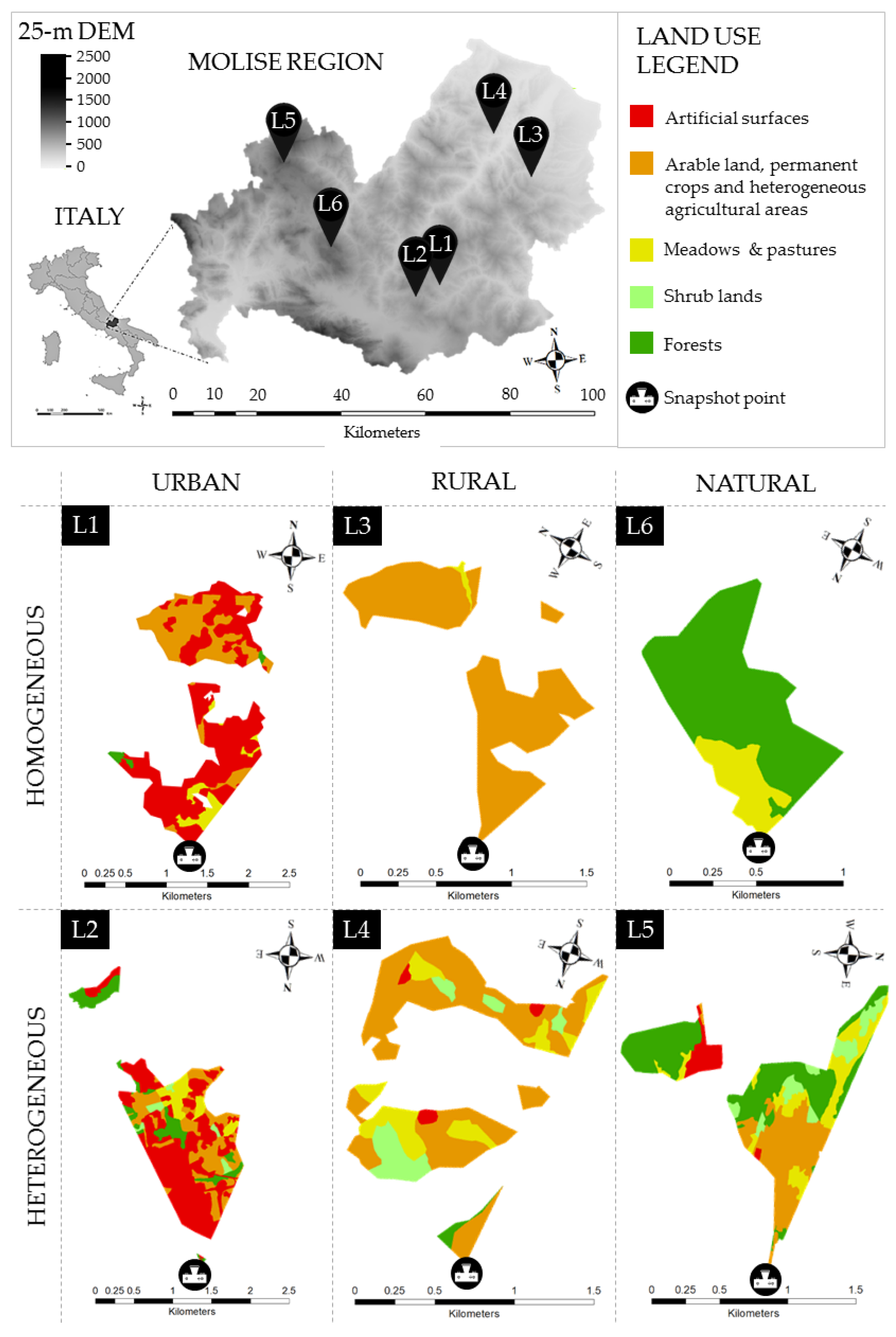
2.1. Land-Use Interpretation

The study was conducted in Molise Region, Central Italy, a Mediterranean region that covers 4461 km² [22] between the Adriatic Sea and the Apennine mountains (Figure 1). The presence of mountains, hills, lowlands and coastal areas in this region fosters the depopulation of marginal districts due to the migration towards areas with better development opportunities. Ecological implications of this demographic and social phenomenon include forest expansion in mountain areas and agricultural intensification and urban expansion in lowlands and along the coast, mostly around the three biggest cities [23,24]. TOF cover 1.7% of the regional territory (7730 ha), having an average patch size of 0.14 ha at 2008 [25]. About 60 tree species were recorded in TOF of the Molise Region, dominated by Quercus pubescens and Quercus cerris, together covering 34% in terms of abundance, followed by Ulmus minor (13%), Acer campestre (8%) and Salix alba (6%). Other species individually contribute to less than 5% in terms of abundance [26].

In order to produce a landscape photo sequence covering the whole urban–rural–natural gradient, a land use interpretation was performed. A sample of 15 oblique photographs, five for each urban, rural and natural landscape domain, was taken along an altitudinal gradient and from representative viewpoints in the Molise region. Photos were taken on sunny days during September 2018. Using a 25 m digital elevation model (DEM), and knowing camera position, orientation, and field of view, we assigned real-world locations to each of the photograph pixels, producing 15 viewsheds, of which we interpreted land-use types. Through the photointerpretation of color aerial orthophotos from 2015 (nominal geometric resolution: 0.5 m), five land-use types have been distinguished and mapped with a minimum mapping unit of 500 m² in order to discriminate TOF: (1) artificial surfaces; (2) arable land, permanent crops and heterogeneous agricultural areas; (3) meadows and pastures; (4) forests; (5) shrublands. These maps were used to calculate three landscape metrics using the “Patch Analyst” tool in the ESRI ArcGIS^® software package. Patch density (PD), land-use class density (CD) and Shannon’s diversity index (SDI) (see [27] for further details on these metrics) were calculated for each viewshed, and then normalized to a 0–1 interval by the min-max method of ranging [28]. Finally, a test for checking the absence of correlation between metrics was performed (Spearman ρ < |0.8|). These metrics were chosen because of their proved correlation with landscape preference [29] as well as their ability to describe landscape structure irrespective of the area extent [30]. The average of these normalized metrics’ values was calculated and assumed as an index of landscape heterogeneity (H index_v) (see

Table A1. Results of the characterization of the 15 viewsheds in relation to main land-use and heterogeneity level. In bold, the six selected viewsheds. Patch density (PD), land-use class density (CD) and Shannon’s diversity index (SDI) and their normalized values, and index of landscape heterogeneity (H index).

ID Photo	Main Land Use	Area (ha)	PD	PD Normalized Value	CD	CD Normalized Value	SDI	SDI Normalized Value	H Index
1	Artificial surfaces	238.1	0.11	0.24	0.017	0.03	0.86	0.61	0.295
2	Artificial surfaces	228.7	0.09	0.17	0.022	0.10	0.89	0.62	0.304
3	Artificial surfaces	99.6	0.20	0.50	0.040	0.37	0.93	0.65	0.515
4	Artificial surfaces	175.2	0.34	0.92	0.023	0.12	0.88	0.62	0.559
5	Artificial surfaces	228.0	0.27	0.71	0.022	0.11	1.24	0.87	0.568
6	Agricultural areas	77.0	0.05	0.07	0.026	0.17	0.07	0.05	0.097
7	Agricultural areas	100.1	0.06	0.09	0.030	0.22	0.20	0.14	0.155
8	Agricultural areas	207.8	0.07	0.13	0.014	0.00	0.75	0.53	0.220
9	Agricultural areas	12.2	0.16	0.40	0.082	1.00	0.00	0.00	0.467
10	Agricultural areas	100.6	0.22	0.56	0.050	0.52	0.98	0.69	0.593
11	Forests	98.6	0.26	0.69	0.051	0.53	1.41	1.00	0.743
12	Forests	101.0	0.19	0.47	0.040	0.37	0.88	0.62	0.489
13	Forests	297.9	0.14	0.33	0.017	0.03	1.00	0.70	0.357
14	Forests	158.0	0.06	0.10	0.025	0.16	0.97	0.68	0.316
15	Forests	71.7	0.03	0.00	0.028	0.19	0.48	0.33	0.178

in Appendix A). Finally, three pairs of photographs, and their related viewsheds, were selected from those showing the lowest and highest H index_v within each landscape domain (urban, rural and natural) (Figure 1). In this way, an urban–rural–natural landscape gradient was recreated as follows:

L1

Homogeneous urban landscape: the landscape with the lowest heterogeneity among those with the main land use represented by artificial surfaces;

L2

Heterogeneous urban landscape: the landscape with the highest heterogeneity among those with the main land use represented by artificial surfaces;

L3

Homogeneous rural landscape: the landscape with the lowest heterogeneity among those with the main land use represented by arable land, permanent crops and heterogeneous agricultural areas;

L4

Heterogeneous rural landscape: the landscape with the highest heterogeneity among those with the main land use represented by arable land, permanent crops and heterogeneous agricultural areas;

L5

Heterogeneous forest landscape: the landscape with the highest heterogeneity among those with the main land use represented by forests;

L6

Homogeneous forest landscape: the landscape with the lowest heterogeneity level among those with the main land use represented by forests.

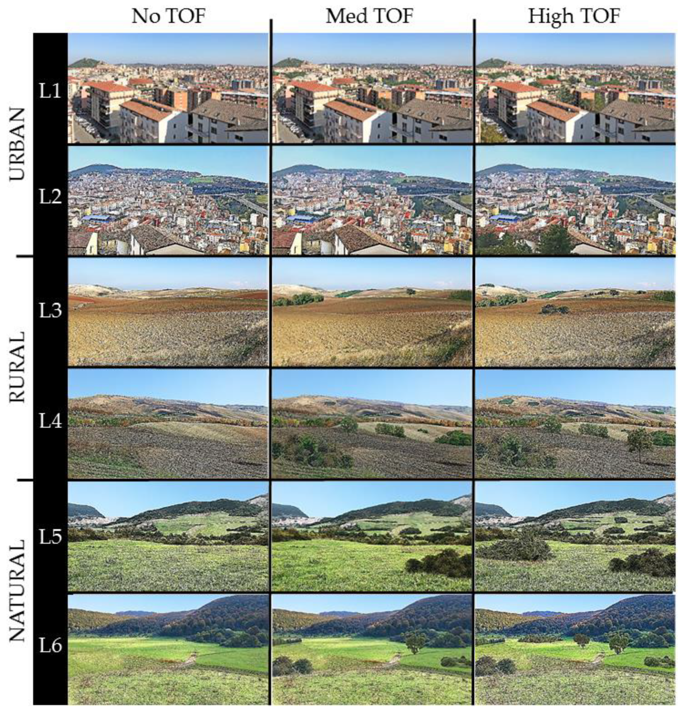
2.2. Visual Choice Experiment

The six selected photos were then modified using a raster graphic editor in order to obtain six triplets of photos each with three different levels of TOF cover (Figure 2). First editing aimed to (i) remove all TOF present in original photos, (ii) harmonize exposure and saturation values, and (iii) eliminate clouds as plausible misleading stimuli on observer perception [31]. Accordingly, the first photo of each triplet referred to the absence of TOF (No TOF). In the second photo of each triplet, TOF was added until covering 1.7% of the viewshed area (Med TOF), which corresponded to the current TOF coverage in Molise region [26]. Finally, the third photo of each triplet was modified by adding TOF elements until reaching a relatively high TOF cover of 3.4% of the viewshed area (High TOF), equal to twice the average value of TOF cover in Molise region. TOF were added within 1.5 km from the snapshot point, as the maximum visual threshold for clearly discerning individual elements such as trees [17].

Edited photos were exhibited in a visual choice experiment to 360 respondents, equally distributed by age, (i.e., “young”, “adults” or “elderly”, respectively between 18 and 35, between 36 and 55, and over 55 years), gender, place of origin (i.e., “inhabitants” or “visitors”) and residential site (i.e., “in town” if their home was within an urban or peri-urban district or “out of town” if their home was in a rural area). Respondents were randomly intercepted in public locations of the Molise Region such as town squares, holiday farms, environmental museums, archaeological sites, ski resorts etc., between December 2018 and March 2019. The first part of interviews included personal information on profession, educational level and marital status. Each respondent was then asked to rank the photos contained in each triplet according to their individual preference. The three photos were simultaneously shown on A2 sheets in order to grant an optimal observation of the landscapes portrayed, facilitating their comparison. Hence, the three photos of each triplet were ranked from 1 to 3 following an increasing aesthetic preference (i.e., 1 for the least preferred, 2 for the intermediate and 3 for the most preferred photo). At the end of the experiment, respondents were asked to rank a sequence composed of the six photos with the Med TOF cover level, assigning an increasing value from 1 to 6 according to increasing aesthetic preference. These values were finally multiplied by the preference values of each photo within the triplet in order to calculate an overall preference score for each of the 18 photos.

The responses were analyzed both on the overall sample and for each individual group of respondents. In order to check the significant differences in preference from different groups of respondents, a χ² test was then performed.

2.3. Landscape Metrics and Landscape Preference Relationships

Corresponding to the photo editing, land-use maps of the six original photos were edited in a GIS environment, thus reproducing the six triplets of viewsheds according to the three TOF cover levels. TOF patches edited in photos were replicated in the corresponding viewsheds, faithfully reflecting their spatial configuration, both for distribution (i.e., azimuth and distance from the observer) and geometry (i.e., shape and area). A landscape analysis of each viewshed was then conducted, computing sixteen landscape metrics commonly used to describe landscape fragmentation, complexity and diversity (see

Table A2. Overview of the 16 landscape metrics [27] originally considered for the landscape analysis of the 18 viewsheds. In bold, the seven metrics selected after the auto-correlation test and used for the landscape analysis.

	Landscape Metric	Acronym	Description
Fragmentation	Patch Density	PD	Number of patches in the viewshed, divided by total viewshed area.
	Mean Patch Size	MPS	Sum, across all patches in the viewshed, of the patch areas, divided by the total number of patches.
	Median Patch Size	MedPS	Area of the patch representing the midpoint of the rank order distribution of patch areas based on all patches in the viewshed.
	Patch Size Coefficient of Variance	PSCoV	Standard deviation of patch areas divided by the mean patch area.
	Patch Size Standard Deviation	PSSD	Square root of the sum of the squared deviations of each patch area from the mean patch area computed for all patches in the viewshed, divided by the total number of patches (i.e., the root mean squared error in the patch size).
	Total Edge	TE	Sum of the lengths of all edge segments in the viewshed.
	Edge Density	ED	Sum of the lengths of all edge segments in the viewshed, divided by the total viewshed.
	Mean Patch Edge	MPE	Lengths of all edge segments in the viewshed divided by the total number of patches.
Complexity	Mean Shape Index	MSI	Sum of patch perimeter divided by the square root of area of each patch in the viewshed, adjusted by a constant for a square standard, divided by the number of patches.
	Area Weighted Mean Shape Index	AWMSI	Sum, across all patches, of each patch perimeter divided by the square root of the patch area, adjusted by a constant for a square standard, multiplied by the patch area and divided by the total area of the viewshed.
	Mean Perimeter-Area Ratio	MPAR	Sum, across all patches in the landscape, of the simple ratio of patch perimeter to area, divided by the total number of patches.
	Mean Patch Fractal Dimension	MPFD	Sum of two times the logarithm of patch perimeter, divided by the logarithm of patch area for each patch in the viewshed, divided by the number of all patches.
	Area Weighted Mean Patch Fractal Dimension	AWMPFD	Sum, across all patches, of two times the logarithm of patch perimeter, divided by the logarithm of patch area multiplied by the patch area divided by the total landscape area.
Diversity	Class Density	CD	Total number of patch classes in the viewshed, divided by total viewshed area.
	Shannon’s Diversity Index	SDI	Sum, across all patch classes, of the proportional cover of each patch class multiplied by that proportion.
	Shannon’s Evenness Index	SEI	Minus the sum, across all patch classes, of the proportional cover of each patch class multiplied by that proportion, divided by the logarithm of the number of patch classes.

in Appendix A). Landscape metrics were calculated through the “Patch Analyst” tool in the ESRI ArcGIS^® software package. Only seven metrics, showing a Spearman ρ < |0.8| between one another, were retained in order to characterize and compare the six different landscapes in relation to the three TOF cover levels. These seven metrics were then normalized to 0–1 range using the min-max method [28]. Normalized metrics were used to calculate three landscape metrics: landscape fragmentation given by the average of mean patch size (MPS), patch size coefficient of variation (PSCoV) and total edge (TE); landscape complexity given by the average of area weighted mean shape index (AWMSI) and mean patch fractal dimension (MPFD); landscape diversity given by the average of class density (CD) and Shannon’s diversity index (SDI). Correlations among the overall preference scores and the three related landscape metrics were then assessed through Pearson’s r correlation analysis. Finally, the statistical significance of the correlations obtained was verified through the t distribution method. We found statistical significance at 0.001 level for all Pearson’s product moment correlation coefficients.

3. Results

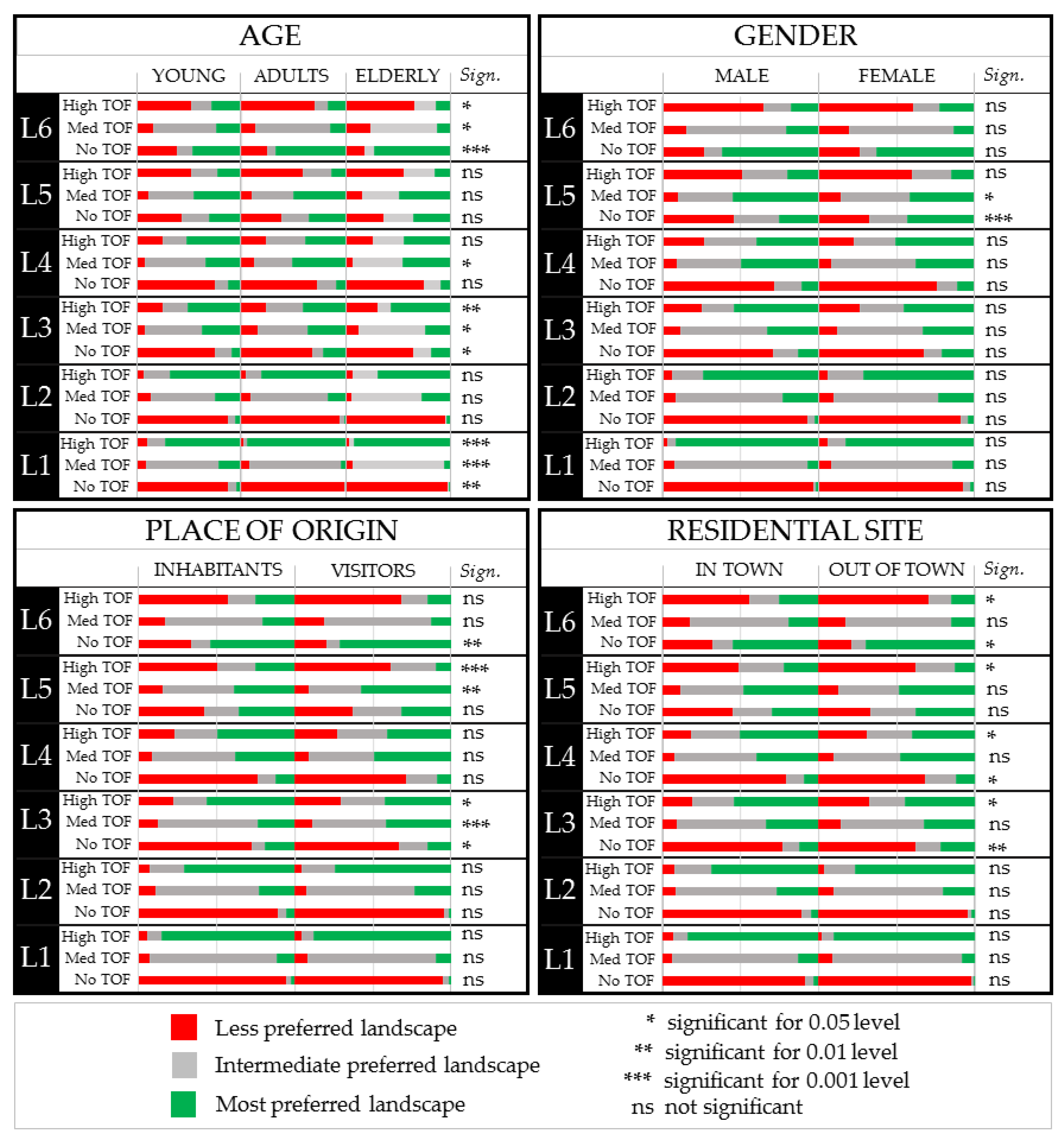
3.1. Visual Choice Experiment

The distributions of preferences were relatively more balanced between different levels of TOF cover in rural and natural landscapes than in the urban ones (

Table 1. Preference distribution of the overall sample of respondents recorded in the visual choice experiment.

Domain	Landscape ID	TOF Cover	Preference Distributions (%)
			Least Preferred Landscape	Intermediate Preferred Landscape	Most Preferred Landscape
URBAN	L1	No TOF	94.4%	3.3%	2.2%
		Med TOF	7.8%	81.4%	10.8%
		High TOF	4.7%	8.3%	86.9%
	L2	No TOF	91.9%	4.4%	3.6%
		Med TOF	9.2%	67.2%	23.6%
		High TOF	5.8%	21.4%	72.8%
RURAL	L3	No TOF	69.2%	13.6%	17.2%
		Med TOF	11.9%	55.0%	33.1%
		High TOF	25.8%	24.4%	49.7%
	L4	No TOF	73.6%	15.6%	10.8%
		Med TOF	8.6%	47.5%	43.9%
		High TOF	24.7%	30.0%	45.3%
NATURAL	L5	No TOF	39.2%	26.7%	34.2%
		Med TOF	12.2%	39.4%	48.3%
		High TOF	55.6%	26.9%	17.5%
	L6	No TOF	26.7%	10.8%	62.5%
		Med TOF	17.5%	65.3%	17.2%
		High TOF	62.8%	16.9%	20.3%

). The results reveal that urban and rural landscapes without TOF are least preferred by most respondents, while those with the highest level of TOF cover are preferred. Conversely, in natural landscapes, most respondents indicate as less preferred those having the highest TOF cover. In fact, preferred natural landscapes are heterogeneous with Med TOF cover and homogeneous without TOF. Slight statistically significant differences appear with respect to the preferences expressed among the different groups of respondents (for further details, see Figure A1 in Appendix A).

3.2. Trees Outside Forests (TOF) Influence on Landscape Structure

The values of landscape metrics with high TOF cover are always higher than medium TOF cover and TOF absence (

Table 2. Values of the seven landscape metrics for the 18 analyzed viewsheds. Mean patch size (MPS), patch size coefficient of variation (PSCoV), total edge (TE), area weighted mean shape index (AWMSI), mean patch fractal dimension (MPFD), class density (CD) and Shannon’s diversity index (SDI).

Domain	Landscape ID	TOF Cover	Fragmentation Metrics			Complexity Metrics		Diversity Metrics
			MPS	PSCoV	TE	AWMSI	MPFD	CD	SDI
URBAN	L1	No TOF	9.2	218.5	44.8	2.88	1.37	0.017	0.86
		Med TOF	6.1	273.1	51.4	3.09	1.40	0.021	0.92
		High TOF	4.1	333.2	58.3	3.39	1.43	0.021	0.96
	L2	No TOF	3.7	293.6	59.1	2.51	1.37	0.022	1.24
		Med TOF	3.0	321.1	67.1	2.87	1.40	0.026	1.30
		High TOF	2.2	368.4	74.0	3.16	1.43	0.026	1.34
RURAL	L3	No TOF	19.3	98.6	9.0	1.78	1.33	0.026	0.07
		Med TOF	9.6	166.8	10.7	1.97	1.38	0.039	0.16
		High TOF	5.9	222.0	12.7	2.21	1.41	0.039	0.22
	L4	No TOF	4.6	170.4	24.9	2.19	1.33	0.050	0.98
		Med TOF	3.6	196.1	27.0	2.27	1.36	0.060	1.05
		High TOF	3.1	209.8	29.0	2.35	1.37	0.060	1.12
NATURAL	L5	No TOF	3.8	164.2	27.8	2.12	1.38	0.051	1.41
		Med TOF	3.0	189.2	30.0	2.22	1.41	0.061	1.45
		High TOF	2.6	202.4	32.0	2.36	1.42	0.061	1.48
	L6	No TOF	35.9	63.5	6.7	1.68	1.29	0.028	0.48
		Med TOF	12.0	179.0	7.5	1.73	1.48	0.042	0.49
		High TOF	7.1	244.9	8.0	1.77	1.46	0.042	0.50

). Accordingly, these metrics’ trends show that a higher TOF cover is directly correlated with a higher level of fragmentation, complexity and diversity of the landscape mosaics. Moreover, differences related to TOF cover are more emphasized in homogeneous than heterogeneous landscapes. In these landscapes (i.e., L1, L3 and L6), MPS, PSCoV and TE show the widest absolute variations in relation to changing TOF cover. In a homogeneous urban landscape (L1), PSCoV and TE increase by 22% and 13% respectively passing from Med TOF to High TOF. At the same time, MPS decreases by 33%. Furthermore, passing from Med TOF to No TOF in L1, PSCoV and TE decrease by 20% and 13%, respectively, and MPS increases by 50%. In homogeneous rural landscape (L3), PSCoV and TE increase by 33% and 19%, respectively, and MPS decreases by 38% for High TOF. While, PSCoV and TE decrease by 41% and 16%, respectively, and MPS increases by 100% passing from Med TOF to No TOF in L3. Lastly, in the homogeneous natural landscape (L6), PSCoV and TE increase by 37% and 7%, respectively, for High TOF and MPS concurrently decreases by 40%. Conversely, passing from Med TOF to No TOF in L6, MPS increases by 200% and PSCoV and TE decrease by 65% and 10%, respectively. In these homogeneous landscapes, we also found that AWMSI and MPFD are less sensitive to changes in TOF cover.

3.3. Correlation between Landscape Metrics and Preferences

Mean preference scores of the 18 photos increase along the urban–rural–natural gradient (

Table 3. Mean preference scores and normalized landscape metrics of the six landscape types investigated in relation to three different levels of TOF cover.

Domain	Landscape ID	TOF Cover	Mean Preference Score	Landscape Fragmentation	Landscape Complexity	Landscape Diversity
URBAN	L1	No TOF	2.1	0.62	0.55	0.28
		Med TOF	3.9	0.75	0.71	0.35
		High TOF	5.1	0.87	0.86	0.36
	L2	No TOF	2.5	0.83	0.46	0.47
		Med TOF	4.6	0.91	0.64	0.55
		High TOF	5.7	1.00	0.80	0.56
RURAL	L3	No TOF	4.9	0.21	0.15	0.10
		Med TOF	6.9	0.39	0.33	0.28
		High TOF	6.7	0.50	0.48	0.30
	L4	No TOF	5.1	0.52	0.26	0.70
		Med TOF	8.8	0.56	0.36	0.83
		High TOF	8.2	0.59	0.40	0.86
NATURAL	L5	No TOF	9.6	0.53	0.37	0.86
		Med TOF	11.6	0.58	0.48	0.99
		High TOF	7.9	0.61	0.55	1.00
	L6	No TOF	12.5	0.00	0.00	0.27
		Med TOF	10.4	0.37	0.51	0.43
		High TOF	8.1	0.49	0.47	0.44

). Furthermore, the increase of the mean preference scores in urban and rural landscape triplets matches the increase of TOF cover. Mean preference scores for L1 and L2 without TOF increase by 85% and 83%, respectively, passing to Med TOF and by 146% and 128% passing to High TOF. Similar, but less emphasized, are the trends related to rural landscape triplets (L3 and L4). Indeed, in these cases, results reveal that the highest mean preference scores correspond to the Med TOF rather than High TOF cover. In fact, in L3 and L4, mean preference scores increase by 142% and 173%, respectively, passing from No TOF to Med TOF, while decrease by 3% and 7% respectively passing from Med TOF to High TOF. Med TOF achieves the highest mean preference score even in the heterogeneous natural landscape (L5) with the lowest value found for High TOF level. For natural homogeneous landscape (L6), No TOF shows the highest mean preference score. In this case, results display a trend in mean preference scores that is opposite to the increase of TOF cover. In detail, mean preference score of L6 decreases by 16% from No TOF to Med TOF and by 23% from Med TOF to High TOF. With regard to the trends of landscape metrics, a direct relation with the increase in TOF cover was found for all landscape types (Table 3). This common trend is particularly emphasized in homogeneous rural and natural landscapes (L3 and L6) where, e.g., landscape diversity triples passing from No TOF to High TOF in L3 and landscape fragmentation rises from 0 to 0.49 passing from No TOF to High TOF in L6.

Main results from the correlation analysis (

Table 4. Mean preference scores and normalized landscape metrics of the six landscape types investigated in relation to three different levels of TOF cover.

	Landscape Preference Scores
	URBAN		RURAL		NATURAL
	L1	L2	L3	L4	L5	L6
Landscape fragmentation	0.62	0.53	0.35	0.43	−0.15	−0.42
Landscape complexity	0.62	0.54	0.33	0.46	−0.14	−0.34
Landscape diversity	0.57	0.55	0.38	0.49	−0.03	−0.37

) show that relationships between trends in mean preference scores and trends in landscape fragmentation, complexity and diversity have greater positive intensity in urban (L1 and L2) than in rural landscapes (L3 and L2). These correlations are inverted, thus becoming negative, passing to natural landscapes (L5 and L6). A homogeneous urban landscape (L1) displays the strongest positive correlations between trends in mean preference scores and trends in landscape metrics, which tend to smoothly decrease passing to a heterogeneous urban landscape (L2). Inversely, positive correlations are stronger in a heterogeneous than in a homogenous rural landscapes (L4 and L3, respectively). A heterogeneous natural landscape (L5) displays very weak correlations, almost null in the case of landscape diversity. Finally, in a homogeneous natural landscape (L6) there are weak negative correlations between mean preference scores and landscape complexity and diversity.

4. Discussion

4.1. Preference along the Urban–Rural–Natural Gradient

Our results demonstrate that preference increases when human-shaped landscapes are rich in TOF. Emotional response to nature amenity is particularly evident in urban domains, where the abundance of natural features (i.e., TOF) are in contrast with the common idea of a townscape. Indeed, as observed by [32], archetypal landscapes generate an immediate judgment by people, which in the specific case of a townscape maximally enriched in natural features (e.g., TOF) reflect in a strong positive consensus. In this sense, our results are in agreement with the theory that landscape preference is commonly increased with exposure to nature [31,33]. Furthermore, the consensus in preferences for urban landscapes is due to the fact that judgment is not only positively conditioned by the cover of natural elements but also negatively influenced by the presence of buildings and modern factories, unanimously recognized as the least appreciated visual landscape elements [34]. The wide agreement between different groups of respondents in preferring high TOF cover in urban contexts indicates that their variations within landscapes are greater than differences in people’s judgments [35]. The changes in preference for TOF depend on the level of landscape naturalness along the urban–rural–natural gradient, resulting as very high in urban domains where TOF represent the last legacy of nature [36]. Our findings are in line with other similar studies, highlighting how people commonly prefer urban landscapes with plentiful natural elements [37,38,39]. Instead, preference analysis in rural landscapes shows a more balanced distribution ratio, albeit confirming the general preference for landscape with high TOF cover. Considering rural landscapes as transitional between extremely anthropized and natural landscapes [40], natural features such as TOF are already present, thus lowering their overall impact compared to urban domains. Indeed, TOF influence on preferences appear slightly greater in homogeneous rural landscapes characterized by high agricultural intensification with respect to heterogeneous and extensively cultivated ones. As shown by [41], trees and small woods in arable plots represent the most appreciated visual landscape attributes. Furthermore, results are consistent with those obtained by [42], showing how preferred elements of the natural landscapes include not only large bio-physical features (i.e., mountains and forests more than TOF) but also conceptual (e.g., wilderness) and emotional (e.g., excitement) aspects. Moreover, [10] proved how in natural landscapes the cover of small and scattered forest patches is interpreted as a reduction in naturalness negatively influencing landscape perception. It is possible that this reaction also depends on the fact that fragmentation of forested landscapes is automatically linked to the spontaneous rewilding of mountain and marginal areas. Indeed, it has been observed that people prefer heterogeneous forested landscapes as long as their heterogeneity is not due to land abandonment [43].

4.2. Effects of Change in TOF Cover and Landscape Metrics

Effects of a change in TOF cover are mostly evident in landscapes with the lowest levels of heterogeneity, where TOF and small patches in general represent the main elements of diversification [5]. Conversely, the ongoing processes of urbanization, agricultural intensification and abandonment of marginal lands in Italy and other countries, are often taking place at the expense of TOF with subsequent landscape homogenization [8]. More specifically, landscape analysis proves how changes in TOF cover in homogeneous landscapes mainly affect patch size and edge metrics. Confirming this result, a spatial simulation exercise by [3] demonstrated that TOF affect this variety of metrics precisely, improving ecological connectivity. Moreover, TOF cover strongly affects diversity metrics in homogeneous rural landscapes where they represent important permanent features of structural and biological diversity [6]. Indeed, agricultural intensification mainly implies the removal of TOF patches to facilitate mechanization, thus favoring the consolidation of small landholdings into single huge proprieties that radically simplify the landscape mosaic [44].

Our results confirm the positive correlations between landscape preferences and landscape metrics in relation to the increasing TOF cover. These correlations are particularly emphasized in landscapes largely modified by humans (i.e., urban and rural). Pearson’s coefficients tend to decrease with the decreasing human-induced landscape alteration in rural compared to urban landscapes. Moreover, landscape diversity is less correlated to preference scores than landscape complexity and fragmentation. As previously mentioned, agricultural lands, currently accounting for almost half of the European Union (EU) surface area [45], have undergone important structural changes in the post-war period, leading to extreme simplification of the landscape mosaics [44]. This simplification also has negative impacts on landscape preference due to the homogenization of the landscape mosaic often dominated by a few and similar large land patches [46]. Moving towards more natural landscapes, human impacts on landscape structure tend to decrease as well as TOF contribution to landscape preference. Although TOF continue to implicate a general upgrading in heterogeneity, preference scores suggest that their increase in natural landscapes is perceived as a reduction of naturalness. Since TOF influence on landscape structure is less marked in heterogeneous natural landscapes compared to homogeneous ones, correlations between trends in preferences and metrics are negligible in the former and weak or medium negative in the latter. In detail, landscape fragmentation shows the highest negative correlation with preference scores in homogeneous natural landscapes (L6), thus confirming fragmentation as a negative indicator for preference in such landscapes [10].

4.3. Methodological Remarks

Our methodology allowed landscape preference for TOF to be assessed along the whole urban–rural–natural gradient. This is particularly relevant to recent objectives of sustainable landscape planning and management highlighting interactions among different services and beneficiaries, but often neglecting the variability of landscape types [47]. In this perspective, the implementation of innovative cross-disciplinary tools able to support landscape planning is foreseeable. Huge efforts in terms of both time and costs needed to assess TOF-related cultural services at large scale through social perception approaches with an adequate level of robustness represent a barrier to their effective implementation in planning strategies [18]. Therefore, it would be more appropriate to advocate techniques that include social information in a biophysical dataset, such as predictive models able to evaluate and map TOF-related cultural services as well as their changes in relation to landscape dynamics [48]. Then again, the development of new indicators based on individual experience in natural environments could facilitate the evaluation of ecological implications on human wellbeing [49]. While these analyses are particularly important to foster in mountain areas, e.g., tourist attractiveness [48], they are becoming crucial in urban areas to promote stress relief and perceived safety linked to greenspaces planning [50]. In this perspective, our results demonstrate that an increasing cover of trees in urban domains, even if in small patches such as TOF, increases landscape preferences. Given that TOF coverage in Italy increased by approximately 27% (91,000 ha) in the last few decades with respect to 1990 [5], it is then crucial to investigate where this change occurred, e.g., natural or urban contexts, in order to understand the impact of such changes on landscape preferences. Moreover, the influence of other aspects such as patch size and shape as well as species composition of TOF elements, might be explored to better characterize their relationship with landscape preferences. These methods would represent the best compromise in order to (i) overcome the conceptual divergence between provisioning and perception of cultural services connected to their intangibility, (ii) incorporate social and ecological bases in sustainable landscape planning and management strategies by optimizing services demand and supply, and (iii) facilitate the implementation of current international recommendations and policies aimed at improving socio-cultural and economic development through green infrastructure and nature-based solutions [51].

5. Conclusions

Our results demonstrate that there is wide agreement among different groups of people in recognizing the added value of TOF to landscape preference. Increasing TOF cover positively affects landscape preferences following a landscape anthropization gradient, thus resulting as higher in urban than rural and natural ecosystems. Accordingly, our findings advocate initiatives aimed at conserving and improving the presence of TOF in urban and rural areas ensuring health, cultural, economic and environmental benefits for people [52]. The positive contribution of TOF on landscape preference in such areas demonstrate that their implementation can also ameliorate this aspect as well as those related to their ecological, regulating and supporting role [53]. In light of our results, we can conclude that increasing tree cover, either by planting or by spontaneous rewilding, even by small patches such as TOF can be considered as a positive initiative to increase landscape preference as well. Otherwise, instead of specific biophysical attributes and features, preference for natural landscapes would seem to be related to emotional reasons, including a transversal perception that originates from cognitive processes. Therefore, TOF contribution to landscape preference is null, if not negative, in extremely natural landscapes where they represent a sort of unwanted human legacy. Considering the influence that landscape preference can play on cultural ecosystem services provisioning and, in turn, on decision making processes, our results can support landscape policy and planning in fostering or hampering TOF diffusion depending on the different territorial contexts. However, given the high variability in the species as well as the spatial composition of TOF, future studies able to combine information on ecological diversity and social perception of this tree resource are suggested.

References

1. De Foresta, H.; Somarriba, E.; Temu, A.; Boulanger, D.; Feuilly, H.; Gauthier, M. Towards the Assessment of Trees Outside Forests: A Thematic Report Prepared in the Framework of the Global Forest Resources Assessment 2010; Food and Agriculture Organization of the United Nations: Rome, Italy, 2013. [Google Scholar]
2. Kleinn, C. On large-area inventory and assessment of trees outside forests. Unasylva 2000, 51, 3–10. [Google Scholar]
3. Rossi, J.P.; Garcia, J.; Roques, A.; Rousselet, J. Trees outside forests in agricultural landscapes: Spatial distribution and impact on habitat connectivity for forest organisms. Landsc. Ecol. 2016, 31, 243–254. [Google Scholar] [CrossRef] [Green Version]
4. Antrop, M. Why landscapes of the past are important for the future. Landsc. Urban Plan. 2005, 70, 21–34. [Google Scholar] [CrossRef]
5. Sallustio, L.; di Cristofaro, M.; Hashmi, M.M.; Vizzarri, M.; Sitzia, T.; Lasserre, B.; Marchetti, M. Evaluating the contribution of Trees Outside Forests and Small Open Areas to the Italian landscape diversification during the last decades. Forests 2018, 9, 701. [Google Scholar] [CrossRef] [Green Version]
6. Sitzia, T.; Trentanovi, G.; Marini, L.; Cattaneo, D.; Semenzato, P. Assessment of hedge stand types as determinants of woody species richness in rural field margins. Iforest Biogeosci. For. 2013, 6, 201–208. [Google Scholar] [CrossRef]
7. Sitzia, T.; Campagnaro, T.; Weir, R.G. Novel woodland patches in a small historical Mediterranean city: Padova, Northern Italy. Urban Ecosyst. 2016, 19, 475–487. [Google Scholar] [CrossRef]
8. Plieninger, T. Monitoring directions and rates of change in trees outside forests through multitemporal analysis of map sequences. Appl. Geogr. 2012, 32, 566–576. [Google Scholar] [CrossRef] [Green Version]
9. Schnell, S.; Altrell, D.; Ståhl, G. The contribution of trees outside forests to national tree biomass and carbon stocks—A comparative study across three continents. Environ. Monit. Assess. 2015, 187, 4197. [Google Scholar] [CrossRef]
10. Ode, Å.; Fry, G.; Tveit, M.S.; Messager, P.; Miller, D. Indicators of perceived naturalness as drivers of landscape preference. J. Environ. Manag. 2009, 90, 375–383. [Google Scholar] [CrossRef]
11. Daniel, T.C. Whither scenic beauty? Visual landscape quality assessment in the 21st century. Landsc. Urban Plan. 2001, 54, 267–281. [Google Scholar] [CrossRef]
12. Appleton, K.; Lovett, A. GIS-based visualisation of rural landscapes: Defining “sufficient” realism for environmental decision-making. Landsc. Urban Plan. 2003, 6, 117–131. [Google Scholar] [CrossRef]
13. Dramstad, W.E.; Tveit, M.S.; Fjellstad, W.J.; Fry, G.L.A. Relationships between visual landscape preferences and map-based indicators of landscape structure. Landsc. Urban Plan. 2006, 78, 465–474. [Google Scholar] [CrossRef]
14. Ode, Å.; Miller, D. Analysing the relationship between indicators of landscape complexity and preference. Environ. Plan. B Plan. Des. 2011, 38, 24–40. [Google Scholar] [CrossRef]
15. Frank, S.; Fürst, C.; Koschke, L.; Witt, A.; Makeschin, F. Assessment of landscape aesthetics-Validation of a landscape metrics- based assessment by visual estimation of the scenic beauty. Ecol. Indic. 2013, 32, 222–231. [Google Scholar] [CrossRef]
16. Sitzia, T.; Dainese, M.; Clementi, T.; Mattedi, S. Capturing cross-scalar variation of habitat selection with grid sampling: An example with hazel grouse (Tetrastes Bonasia L.). Eur. J. Wildl. Res. 2014, 60, 177–186. [Google Scholar] [CrossRef]
17. Schirpke, U.; Tasser, E.; Tappeiner, U. Predicting scenic beauty of mountain regions. Landsc. Urban Plan. 2013, 111, 1–12. [Google Scholar] [CrossRef]
18. Schirpke, U.; Timmermann, F.; Tappeiner, U.; Tasser, E. Cultural ecosystem services of mountain regions: Modelling the aesthetic value. Ecol. Indic. 2016, 69, 78–90. [Google Scholar] [CrossRef] [PubMed] [Green Version]
19. Boll, T.; Von Haaren, C.; Von Ruschkowski, E. The preference and actual use of different types of rural recreation areas by urban dwellers—The Hamburg case study. PLoS ONE 2014, 9, e108638. [Google Scholar] [CrossRef] [Green Version]
20. Vizzari, M.; Sigura, M. Landscape sequences along the urban-rural-natural gradient: A novel geospatial approach for identification and analysis. Landsc. Urban Plan. 2015, 140, 42–55. [Google Scholar] [CrossRef]
21. Schirpke, U.; Tappeiner, G.; Tasser, E.; Tappeiner, U. Using conjoint analysis to gain deeper insights into aesthetic landscape preferences. Ecol. Indic. 2019, 96, 202–212. [Google Scholar] [CrossRef]
22. Istituto Nazionale di Statistica (ISTAT) Principali Dimensioni Geostatistiche e Grado di Urbanizzazione del Paese. Available online: https://www.istat.it/it/archivio/137001 (accessed on 20 May 2020).
23. Sallustio, L.; Quatrini, V.; Geneletti, D.; Corona, P.; Marchetti, M. Assessing land take by urban development and its impact on carbon storage: Findings from two case studies in Italy. Environ. Impact Assess. Rev. 2015, 54, 80–90. [Google Scholar] [CrossRef] [Green Version]
24. Marchetti, M.; Vizzarri, M.; Sallustio, L.; di Cristofaro, M.; Lasserre, B.; Lombardi, F.; Giancola, C.; Perone, A.; Simpatico, A.; Santopuoli, G. Behind forest cover changes: Is natural regrowth supporting landscape restoration? Findings from central Italy. Plant Biosyst. An Int. J. Deal. Asp. Plant Biol. 2018, 152, 524–535. [Google Scholar] [CrossRef]
25. Fattorini, L.; Puletti, N.; Chirici, G.; Corona, P.; Gazzarri, C.; Mura, M.; Marchetti, M. Checking the performance of point and plot sampling on aerial photoimagery of a large-scale population of trees outside forests. Can. J. For. Res. 2016, 46, 1264–1274. [Google Scholar] [CrossRef]
26. Marchetti, M.; Garfì, V.; Pisani, C.; Franceschi, S.; Marcheselli, M.; Corona, P.; Puletti, N.; Vizzarri, M.; di Cristofaro, M.; Ottaviano, M.; et al. Inference on forest attributes and ecological diversity of trees outside forest by two-phase inventory. Ann. For. Sci. 2018, 75, 37. [Google Scholar] [CrossRef] [Green Version]
27. McGarigal, K. Landscape pattern metrics. In Wiley StatsRef: Statistics Reference Online; Balakrishnan, N., Colton, T., Everitt, B., Piegorsch, W., Ruggeri, F., Teugels, J.L., Eds.; John Wiley & Sons, Ltd.: New York, NY, USA, 2014. [Google Scholar]
28. Sneath, P.H.A.; Sokal, R.R. Numerical Taxonomy—The Principles and Practice of Numerical Classification; W. H. Freeman and Company: New York, NY, USA, 1973. [Google Scholar]
29. Uuemaa, E.; Antrop, M.; Roosaare, J.; Marja, R.; Mander, Ü. Landscape metrics and indices: An overview of their use in landscape research. Living Rev. Landsc. Res. 2009, 3, 1–28. [Google Scholar] [CrossRef]
30. Plexida, S.G.; Sfougaris, A.I.; Ispikoudis, I.P.; Papanastasis, V.P. Selecting landscape metrics as indicators of spatial heterogeneity—A comparison among Greek landscapes. Int. J. Appl. Earth Obs. Geoinf. 2014, 26, 26–35. [Google Scholar] [CrossRef]
31. Kaplan, R.; Kaplan, S. The Experience of Nature: A Psychological Perspective; Cambridge University Press: Cambridge, UK, 1989. [Google Scholar]
32. Hagerhall, C.M. Consensus in landscape preference judgements. J. Environ. Psychol. 2001, 21, 83–92. [Google Scholar] [CrossRef]
33. Kellert, S.R.; Wilson, E.O. The Biophilia Hypothesis; Island Press: Washington, DC, USA, 1995. [Google Scholar]
34. Tempesta, T.; Vecchiato, D. Testing the difference between experts’ and lay people’s landscape preferences. Aestimum 2015, 66, 1–41. [Google Scholar]
35. Daniel, T.C. Measuring Landscape Esthetics: The Scenic Beauty Estimation Method; Department of Agriculture, Forest Service, Rocky Mountain Forest and Range Experiment Station: Fort Collins, CO, USA, 1976; Volume 167.
36. Willis, K.J.; Petrokofsky, G. The natural capital of city trees. Science 2017, 356, 374–376. [Google Scholar] [CrossRef]
37. Vesely, É.T. Green for green—The perceived value of a quantitative change in the urban tree estate of New Zealand. Ecol. Econ. 2007, 63, 605–615. [Google Scholar] [CrossRef]
38. Camacho-Cervantes, M.; Schondube, J.E.; Castillo, A.; MacGregor-Fors, I. How do people perceive urban trees? Assessing likes and dislikes in relation to the trees of a city. Urban Ecosyst. 2014, 17, 761–773. [Google Scholar] [CrossRef]
39. Giergiczny, M.; Kronenberg, J. From valuation to governance: Using choice experiment to value street trees. Ambio 2014, 43, 492–501. [Google Scholar] [CrossRef] [PubMed] [Green Version]
40. Colgan, C.; Hunter, M.L., Jr.; McGill, B.; Weiskittel, A. Managing the middle ground: Forests in the transition zone between cities and remote areas. Landsc. Ecol. 2014, 29, 1133–1143. [Google Scholar] [CrossRef] [Green Version]
41. Van Zanten, B.T.; Zasada, I.; Koetse, M.J.; Ungaro, F.; Häfner, K.; Verburg, P.H. A comparative approach to assess the contribution of landscape features to aesthetic and recreational values in agricultural landscapes. Ecosyst. Serv. 2016, 17, 87–98. [Google Scholar] [CrossRef]
42. Beza, B.B. The aesthetic value of a mountain landscape: A study of the Mt. Everest Trek. Landsc. Urban Plan. 2010, 97, 306–317. [Google Scholar] [CrossRef]
43. Vecchiato, D.; Tempesta, T. Valuing the benefits of an afforestation project in a peri-urban area with choice experiments. For. Policy Econ. 2013, 26, 111–120. [Google Scholar] [CrossRef]
44. Eichhorn, M.P.; Paris, P.; Herzog, F.; Incoll, L.D.; Liagre, F.; Mantzanas, K.; Mayus, M.; Moreno, G.; Papanastasis, V.P.; Pilbeam, D.J.; et al. Silvoarable Systems in Europe–Past, Present and Future Prospects. Agrofor. Syst. 2006, 67, 29–50. [Google Scholar] [CrossRef]
45. FAOSTAT Land Use Database. Available online: http://www.fao.org/faostat/en/#data/RL/visualize (accessed on 15 May 2020).
46. Svobodova, K.; Sklenicka, P.; Vojar, J. How does the representation rate of features in a landscape affect visual preferences? A case study from a post-mining landscape. Int. J. Min. Reclam. Environ. 2015, 29, 266–276. [Google Scholar] [CrossRef]
47. Dronova, I. Landscape beauty: A wicked problem in sustainable ecosystem management? Sci. Total Environ. 2019, 688, 584–591. [Google Scholar] [CrossRef] [Green Version]
48. Schirpke, U.; Altzinger, A.; Leitinger, G.; Tasser, E. Change from agricultural to touristic use: Effects on the aesthetic value of landscapes over the last 150 years. Landsc. Urban Plan. 2019, 187, 23–35. [Google Scholar] [CrossRef]
49. Johansson, M.; Pedersen, E.; Weisner, S. Assessing cultural ecosystem services as individuals’ place-based appraisals. Urban For. Urban Green. 2019, 39, 79–88. [Google Scholar] [CrossRef]
50. Campagnaro, T.; Vecchiato, D.; Arnberger, A.; Celegato, R.; Da Re, R.; Rizzetto, R.; Semenzato, P.; Sitzia, T.; Tempesta, T.; Cattaneo, D. General, stress relief and perceived safety preferences for green spaces in the historic city of Padua (Italy). Urban For. Urban Green. 2020, 52, 126695. [Google Scholar] [CrossRef]
51. Lafortezza, R.; Sanesi, G. Nature-based solutions: Settling the issue of sustainable urbanization. Environ. Res. 2019, 172, 394–398. [Google Scholar] [CrossRef] [PubMed]
52. Sallustio, L.; Perone, A.; Vizzarri, M.; Corona, P.; Fares, S.; Cocozza, C.; Tognetti, R.; Lasserre, B.; Marchetti, M. The green side of the grey: Assessing greenspaces in built-up areas of Italy. Urban For. Urban Green. 2019, 37, 147–153. [Google Scholar] [CrossRef]
53. Marando, F.; Salvatori, E.; Sebastiani, A.; Fusaro, L.; Manes, F. Regulating ecosystem services and green infrastructure: Assessment of urban heat island effect mitigation in the municipality of Rome, Italy. Ecol. Mod. 2019, 392, 92–102. [Google Scholar] [CrossRef]
Figure 1. The six selected viewsheds representative of the urban–rural–natural landscape gradient and their geographical location in the study area.
Forests 11 00728 g001
Figure 2. The six triplets of photos edited with a raster graphic editor, showing six different landscape types of the urban–rural–natural gradient (from top to bottom) and three increasing trees outside forests (TOF) covers (from left to right).
Forests 11 00728 g002