Application of a Negative Multinomial Model Gives Insight into Rarity-Area Relationships

Abstract

The distribution of individuals of different species across different sampling units is typically non-random. This distributional non-independence can be interpreted and modelled as a correlated multivariate distribution. However, this correlation cannot be modelled using a totally independent and random distribution such as the Poisson distribution. In this study, we utilized the negative multinomial distribution to overcome the problem encountered by the commonly used Poisson distribution and used it to derive insight into the implications of field sampling for rare species’ distributions. Mathematically, we derived, from the negative multinomial distribution and sampling theory, contrasting relationships between sampling area, and the proportions of locally rare and regionally rare species in ecological assemblages presenting multi-species correlated distribution. With the suggested model, we explored the cross-scale relationships between the spatial extent, the population threshold for defining the rarity of species, and the multi-species correlated distribution pattern using data from two 50-ha tropical forest plots in Barro Colorado Island (Panama) and Heishiding Provincial Reserve (Guangdong Province, China). Notably, unseen species (species with zero abundance in the studied local sample) positively contributed to the distributional non-independence of species in a local sample. We empirically confirmed these findings using the plot data. These findings can help predict rare species–area relationships at various spatial scales, potentially informing biodiversity conservation and development of optimal field sampling strategies.

1. Introduction

For better conservation of biological diversity, ecologists have explored the spatial distribution patterns of rare species. A variety of ecological mechanisms can contribute to species rarity; for example, habitat heterogeneity, dispersal limitation, and pest-pressure hypothesis [1,2,3]. However, the general relationship between species rarity and non-independence of species distribution remains to be explored [3,4,5].

The definition of distributional non-independence or non-randomness can be multifaceted, some tangible forms of which can be aggregated distribution [6,7], regular distribution or correlated distribution [8]. For the multivariate framework that will be employed here, we interpret the term distributional non-independence as a correlated multivariate distribution. That is, distribution of individuals of different species across different quadrats presents some degree of correlation [8]. Therefore, if some species present aggregate (random or regular) distributions, because of the multivariate correlation effect, it is also expected that other species in the assemblage also present aggregate (random or regular) distribution. This positive correlation cannot be predicted by totally independent and random distribution models (i.e., the Poisson model) [6,7,8]. For the tropical and subtropical forest plots investigated below, a positive correlated distribution was confirmed. Moreover, it has been observed that the multi-species correlated distribution should present a mixed pattern of aggregate and random distributions of different species [8]. However, as mentioned above, the relationship between the correlated distribution of the entire ecological assemblage and rare species distribution is totally unclear, even though the relationship between the abundance variability and distributional aggregation, as one form of distributional non-independence, has been well explored at the species level [9,10]. Finally, the scale dependency effect using quadrat sampling further obscures the general relationship between the two quantities.

Empirically, at a species level, rare species show more spatially aggregated distribution compared with common tree species in both temperate and tropical forests [4,5,9,11]. However, the relationship may be more complex than previously thought as the definition of rare species is relative, somewhat arbitrary, and related to some abundance thresholds [12,13,14,15,16]. For example, a variety of rarity threshold rules are employed to classify rare species in the studied assemblages [12,13,14].

Other than the species abundance threshold, it is also important to recognize that the spatial extent of studied areas also influences the definition of rare species in community ecology [16]. This is particularly true when conducting local sampling or surveys of ecological assemblages in a large region or habitat. How should we define a rare species? If a limited local sampling can survey only 10% of the whole region at the local scale, we may argue that species A is rare when its individuals have a number of 5 based on the surveyed area, in comparison to a reference species B that has 100 individuals in the surveyed area. However, if species A has a much more aggregated distribution and has 10,000 individuals in the remaining 90% unsampled part of the region, while the distribution of species B is fully random with 900 individuals in the remaining area, then species B (total population size = 1000), at the regional scale, is definitely much rarer than species A (total population size = 10,005). Therefore, when studying scale-related species rarity patterns, it is necessary to clearly define the corresponding sampling spatial extent and the population threshold [16].

Moreover, if the studied assemblage has more rare species, then the corresponding species abundance distribution should become more right skewed in the curve shape (i.e., abundances of most species tend to concentrate at small values while the other species are highly abundant, which results in the abundance distribution displaying a long right-tailed pattern), which would result in a large variation of species abundance. As such, if a positive relationship is observed between population rarity and non-random distribution of a species, then a systematic association should be expected between the abundance variability and distributional non-independence of the entire assemblage.

An important factor that can hinder the progress of earlier work in evaluating the relationships between non-independence, variability, and rarity is related to the statistical methods used in these studies. The independent negative binomial distribution (NBD) statistical model was widely used for describing aggregated distribution of a single species [6,17,18,19,20,21]. However, the species-specific NBD model does not consider that the distribution of individuals of a species in different sampling quadrats may be non-random and spatially dependent.

In summary, in our present study, a multivariate statistical model negative multinomial model (NMM) is used to describe assemblage-level correlated distribution patterns to evaluate the relationship between species rarity, non-independent distribution, and abundance variability (quantified by the coefficient of variation, CV) patterns. Based on the NMM-induced assemblage-level correlated distribution and the context of the sampling theorem, we derived the theoretical sampling theory for two forms of rarity, locally rare species and regionally rare species, with respect to the changing sampling area fraction.

In our study, we define locally rare species are those with an abundance not greater than a rarity threshold in the local sample, while regionally rare species are defined by their abundances (the total number of individuals spread over the entire forest plot) being not greater than the same rarity threshold. Two permanent tropical forest plots were analysed for testing the empirical deviation from the theoretical expectation. We confirmed that locally rare species and regionally rare species presented nearly opposite mirror-like curve patterns when the sampling size of the local quadrat increased. Finally, we also showed that neighbouring unseen species can have impacts on the estimation of the assemblage-level correlated distribution.

Our central goal of conducting such analyses is to better characterize multi-species distributional non-randomness patterns using a multivariate model for theoretically deriving and empirically verifying two different forms of rare species–area relationships. The findings at the forest-plot scales provided in the study can be used to extrapolate rare species diversity at larger spatial scales to better inform global and regional biodiversity conservation and to interpolate rare species diversity at smaller spatial scales.

2. Materials and Methods

In the following section, we built an NMM to capture the correlated multivariate distribution patterns of the individuals of species across different sampling quadrats. For modelling simplicity, we will assume different species in an assemblage sharing the same statistical parameters in the modelling. Throughout the paper, we define unseen species as those species with zero abundance in the locally sampled area but which could be observed elsewhere when the studied region is expanded to cover more neighbouring areas. Even though we did not explicitly study endemic species that are important and essential for biodiversity conservation [22,23], those regionally rare species investigated here are very likely to be endemic when sampling grain sizes are sufficiently large to cover all individuals of these species.

2.1. The Negative Multinomial Model

A region with an area size A (e.g., the area size of the entire forest plot in our empirical tests) has S species. The abundances of these S species are denoted by $N_{1,A},N_{2,A},\dots ,N_{S,A}$, each of which is assumed to follow an NBD whose probability function is as follows [8,20,21]:

$$P(N_{i,A}=n|k,u)=\frac{\Gamma (k+n)}{\Gamma (n+1)\Gamma (k)}{\left(\frac{u}{u+A}\right)}^k{\left(\frac{A}{u+A}\right)}^n,$$

(1)

where k represents a shape parameter measuring non-independence of the spatial distribution of individuals of a species (k > 0). In a single-species setting, a large k indicates a reduced aggregation of organisms (i.e., their distribution tends to be more random) and vice versa. Under the multivariate setting that will be discussed below, this shape parameter k was used to model the strength of positively correlated distributions of different species across different sampling quadrats. A large (or small) k indicates that the positive correlation strength of multiple species’ distributions becomes weak (or strong), implying that the degree of assemblage-level distributional non-independence or non-randomness is weak (or strong). Finally, the parameter u is reciprocally related to the mean population abundance of the NBD model for fixed values of both k and area size A, which is $E(N_{i,A})=Ak/u$, and it is also related to the variance of the model as follows: $Var(N_{i,A})=Ak(A+u)/u^2$. A low u implies a high density of species populations per unit of sampling area.

Based on Equation (1), the CV of species abundance at the spatial scale of the entire region A is a function of both k and u and can be explicitly expressed as follows:

$$C{V}_A=\sqrt{\frac{Var(N_{i,A})}{E^2(N_{i,A})}}=\sqrt{\frac{A+u}{Ak}},$$

(2)

This relationship implies that species in ecological communities with a high variability of species abundance tend to have a strong level of multi-species correlated distribution based on the reciprocal relationship between CV and k (if other parameters A and u are fixed in Equation (2)).

For sampling convenience, the region is divided into q quadrats, with areas $a_1, a_2,\dots , a_q$ and $A={\displaystyle {\sum }_{i=1}^q{a}_i}$. Note that the sizes of $a_1, a_2,\dots ,a_q$ could be different. Let $N_{i1},N_{i2},\dots ,N_{iq}$ denote the corresponding numbers of individuals of species i scattered over these q quadrats. When the total abundance of species i ($N_{i,A}={\displaystyle {\sum }_{j=1}^q{N}_{ij}}$) is determined, a natural assumption for $N_{i1},N_{i2},\dots ,N_{iq}$ is to enforce a multinomial distribution as follows:

$$P(N_{i1}=n_1,\dots ,N_{iq}=n_q|N_{i,A}=n)=\frac{n!}{{\displaystyle {\prod }_{j=1}^q{n}_j!}}{{\displaystyle \prod _{j=1}^q\left(\frac{a_j}{A}\right)}}^{n_j},$$

(3)

Because $N_{i,A}$ follows NBD as in Equation (1), the unconditional joint distribution of $N_{i1},N_{i2},\dots ,N_{iq}$ is a negative multinomial distribution (NMD) as follows [21]:

$$P(N_{i1}=n_1,\dots ,N_{iq}=n_q|k,u)=\frac{\Gamma \left(k+{\displaystyle {\sum }_{j=1}^q{n}_j}\right)}{\Gamma (k){\displaystyle {\prod }_{j=1}^q\Gamma (n_j+1)}}{\left(\frac{u}{u+A}\right)}^k{\displaystyle \prod _{j=1}^q{\left(\frac{a_j}{u+A}\right)}^{n_j}},$$

(4)

The model derived from Equation (4) (which is NMM) describes the multi-species spatial distributional patterns over different quadrats of the studied region at the assemblage level. When the shape parameter k value is very small (or very large), the positive correlated distributions of individual species tend to be strong (or weak) and accordingly, the abundance variability (measured by CV in Equation (2)) will be high (or low).

However, if $N_{i,A}$ (at the whole assemblage level) follows a random distribution (i.e., Poisson model with intensity $A\lambda$ and probability function $P(N_{i,A}=n|\lambda )=e^{-A\lambda }{\left(A\lambda \right)}^n/n!$), then the unconditional distribution of $N_{i1},N_{i2},\dots ,N_{iq}$ (species level) is expressed as follows:

$$P(N_{i1}=n_1,\dots ,N_{iq}=n_q|\lambda )={\displaystyle \prod _{j=1}^q\frac{e^{-a_j\lambda }{\left(a_j\lambda \right)}^{n_j}}{\Gamma (n_j+1)}},$$

(5)

which indicates the abundances of species i scattered over q quadrats, following independent and random Poisson distributions. The detailed derivation of Equation (5) is shown in the Additional Methods of the Supporting Information.

When a local area a is surveyed within region A, then the model in Equation (4) can be refined as a negative trinomial distribution (NTD):

$$P(N_{i,a}=x,N_{i,A-a}=y|k,u)=\frac{\Gamma (k+x+y)}{\Gamma (x+1)\Gamma (y+1)\Gamma (k)}{\left(\frac{u}{u+A}\right)}^k{\left(\frac{a}{u+A}\right)}^x{\left(\frac{A-a}{u+A}\right)}^y,$$

(6)

where $N_{i,a}$ is the number of individuals of species i in the local area a; x and y are two nonnegative integers with $x+y\ge 0$. Note that all species share the same parameters k and u because they are distributed in the same region and are affected by similar environmental factors. The marginal distribution of N_i,a is derived from the model in Equation (6) as follows:

$$P(N_{i,a}=n|k,u)=\frac{\Gamma (k+n)}{\Gamma (n+1)\Gamma (k)}{\left(\frac{u}{u+a}\right)}^k{\left(\frac{a}{u+a}\right)}^n,n\ge 0.$$

(7)

For the derivation of Equation (7) from the NTD in detail above, please refer to the Additional Methods of the Supporting Information. After a simple transformation, this form is identical to the conventional negative binomial probability model used in previous studies [6,17,24]. At the spatial scale when the sampling quadrat has a size of a, the corresponding population mean is $E(N_{i,a})=ak/u$, variance $Var(N_{i,a})=ak(a+u)/u^2$, and CV $C{V}_a=\sqrt{(a+u)/(ak)}$.

2.2. Parameter Estimation

Let $f_m={\displaystyle {\sum }_{i=1}^{S}I(N_{i,a}=m)}$ denote the number of species with m individuals in the sampled assemblage; thus, (f₁, f₂, ..., f_τ) follows a multinomial distribution with a total number of species S over the entire region A and cell probabilities $({\rho }_1,{\rho }_2,\dots ,{\rho }_{\tau })$, where ${\rho }_n=P(N_{i,a}=n|k,u)$ for a local sample $a\subseteq A$ and $\tau =max\{N_{1,a},N_{2,a},\dots ,N_{S,a}\}$; therefore, the likelihood function is expressed as follows:

$$L(k,u|f_1,\dots ,f_{\tau })=\frac{\left({\displaystyle {\sum }_{j=1}^{\tau }{f}_j}\right)!}{{\displaystyle {\prod }_{j=1}^{\tau }{f}_j!}}{\displaystyle \prod _{j=1}^{\tau }{\left(\frac{{\rho }_j}{1-{\rho }_0}\right)}^{f_j}},$$

(8)

which is viewed as a conditional likelihood function based on the observed number of species, ${\displaystyle {\sum }_{j=1}^{\tau }{f}_j}$, in the local sample. Analogous applications can be found in previous studies [21,25,26,27].

The maximum likelihood estimators $\widehat{k}$ and $\widehat{u}$ of $k$ and $u$ can be solved by maximizing the likelihood function in Equation (8). We place all species in the likelihood model, and only a pair of $\widehat{k}$ and $\widehat{u}$ is obtained. The variances of the parameters are calculated using the observed information matrix, and the details are presented in the Supporting Information (Equation (S1)). Additionally, for computing convenience, the R code for calculating the maximum likelihood estimates of $k$ and $u$, their estimated standard errors, and corresponding 95% confidence intervals is provided in the Supporting Information.

In this likelihood function, we controlled the potential effect of unseen species ${\rho }_0$ by normalizing ${\rho }_i (i=1,2,\dots ,\tau )$ with the sum as one. As a comparison, we also presented an alternative likelihood function without accounting for the influence of unseen species ${\rho }_0$ (Supporting Information Equation (S2)) and fitted the corresponding parameter values. Our results show that the strength of distributional non-independence is weaker when the effect of unseen species ${\rho }_0$ exists.

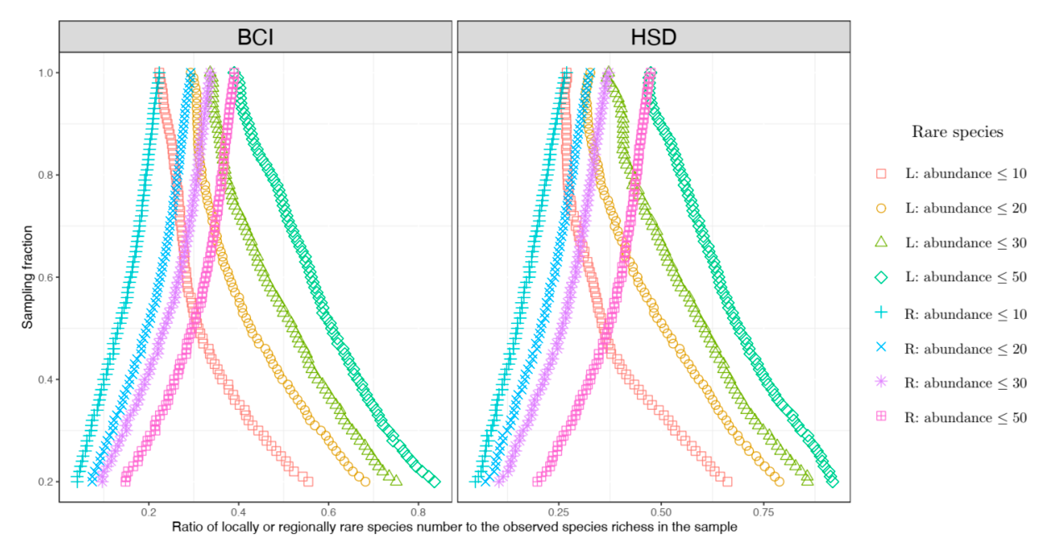
To unravel the general relationships between locally rare species, regionally rare species, and sampling fractions of local area sizes, based on the formulae of NMD or NTD (Equation (4) or (6)), the expected ratio of locally rare species to the observed species numbers can be approximately expressed as follows:

$$P_L=\frac{{\sum }_{i=1}^S{\sum }_{j=1}^{k}P\left(N_{i,a}=j\right)}{{\sum }_{i=1}^{S}P(N_{i,a}>0)}=\frac{{\sum }_{j=1}^k\frac{\Gamma \left(k+j\right)}{\Gamma \left(j+1\right)\Gamma \left(k\right)}{\left(\frac{u}{u+a}\right)}^k{\left(\frac{a}{u+a}\right)}^j}{\left(1-{\left(\frac{u}{u+a}\right)}^k\right)},$$

(9)

where $k$ represents the abundance threshold for rare species (which is 10, 20, 30 or 50 as mentioned above).

As a comparison, the expected ratio of regionally rare species to the observed species numbers can be approximately expressed as follows:

$$P_R=\frac{{\sum }_{i=1}^S{\sum }_{j=1}^{k}P\left(N_{i,a}=j,N_{i,A-a}=0\right)}{{\sum }_{i=1}^{S}P\left(N_{i,a}>0\right)}=\frac{{\sum }_{j=1}^k\frac{\Gamma \left(k+j\right)}{\Gamma \left(j+1\right)\Gamma \left(k\right)}{\left(\frac{u}{u+a}\right)}^k{\left(\frac{a}{u+a}\right)}^j{\left(\frac{u+a}{u+A}\right)}^{k+j}}{\left(1-{\left(\frac{u}{u+a}\right)}^k\right)},$$

(10)

By comparing Equations (9) and (10), one can see that because ${\left(\frac{u+a}{u+A}\right)}^{k+j}\le 1$ obviously holds for $a\le A$, $P_R\le P_L$ across different sampling fractions is always true. The equality becomes true only when $a=A$ (i.e., the sampling fraction $a/A=1$).

2.3. Empirical Tests

Two forest-plot datasets from tropical areas were employed as sampling populations to evaluate the assemblage-level relationships among the species abundance rarity, and variability and distributional non-independence across various spatial sampling scales. The Barro Colorado Island (BCI) plot is located in Panama, Central America, and has a size of 50 ha (1000 × 500 m) [28,29,30,31,32]. The BCI plot has been canvassed eight times, and the data used here were collected in 2005, which showed that it contained 208,383 trees (diameter at breast height ≥1 cm) and 300 species. The Heishiding (HSD; 50 ha; 2011 census) plot located within the Heishiding Provincial Reserve in Guangdong Province of China [33] contains 156 species identified from 37,858 individuals (diameter at breast height ≥10 cm).

To evaluate the multiscale relationships among species rarity, abundance variability, and non-independence at the assemblage level, we conducted a multiscale sampling scheme to randomly sample local communities from small to large until the entire forest plot was accounted for. To be specific, at each given spatial grain scale (or quadrat size), 100 local communities were randomly sampled. This was done by randomly placing 100 quadrats with the same grain size inside the forest plot. These quadrats may or may not have overlapped, depending on the size of sampling quadrat placed inside the forest plot. Note that, in this random sampling process, it was ensured that the entire region of each of the 100 quadrats was fully covered by the forest plot to avoid edge effects.

For each of these 100 randomly sampled local communities (i.e., the composition of species at each spatial sampling scale less than the size of the entire plot), we calculated or measured the following quantities: (1) degree of assemblage non-independence, which is reflected by the estimated shape parameter k for each local assemblage; (2) the size of the local assemblage, which is the number of individuals of all species found in the local assemblage; (3) percent of locally rare species, which is the percent of species with abundances of less than 10, 20, 30 or 50 found in the local assemblage relative to the total number of species found in the local assemblage; (4) percent of regionally rare species, which is the percent of species with abundances of less than 10, 20, 30 or 50 found at the entire forest plot level (e.g., BCI as a whole) relative to the total number of species found in the local assemblage; and (5) abundance variability, which is represented by the estimated CV_a for the species abundance distribution in the local assemblage. It is worth noting that the above definition of locally and regionally rare species was not ad hoc, as each was studied separately in the previous empirical literature [34,35,36,37,38].

The averages of these quantities for 100 randomly sampled assemblages were taken to represent the overall non-randomness degree and abundance variability at that scale. Our analyses were multiscale, since we analysed many spatial scales (or quadrat sizes) from small to large for each forest plot to show crossing-scale patterns, i.e., the range of sampling spatial scales for both plots was from 20,000 m² to 500,000 m².

3. Results

Our empirical applications (

Table 1. Estimated values of k and u and their 95% confidence intervals (CI) and CV and the corresponding maximal log-likelihood values (ln L(k,u)) for the two forest plots based on Equation (8). For the Barro Colorado Island (BCI) plot and the Heishiding (HSD) plot, the whole plot size was the same as A = 50 ha.

Plot	k		u		CVA	ln L(k,u)
	Estimate	95% CI	Estimate	95% CI
BCI	0.10031	(0.05, 0.15)	0.01281	(0.008, 0.017)	3.16	−694.8
HSD	0.16445	(0.07, 0.26)	0.04990	(0.028, 0.072)	2.47	−349.6

) showed that the interspecific distribution of tree species in the HSD forest plot was less positively correlated (k = 0.16445), while the tree distributions were more correlated in the BCI plot in Panama, which had a corresponding k value of 0.1003. By contrast, regarding the comparison of the two CVs, the BCI forest plot had a higher value than the HSD plot. Finally, the estimated u in the BCI plot was lower (implying a high density of species populations per unit of sampling area) than that in the HSD plot (Table 1). Across the different sampling scales, the fitted k and u values were positively correlated at the assemblage level (Figure S1).

Theoretically, when parameter u is fixed, a higher k would result in a lower probability of being rare (i.e., having a small population size ≤10, 20, or 30) for a single species (Figure 1). By contrast, when parameter k is fixed, a lower mean abundance of a species (higher u) will result in a higher probability of being rare (i.e., having a small population size ≤10, 20, or 30) for a single species (Figure S2). This is expected given that u is inversely related to the mean population density of a species; a higher u implies that the sampled assemblage is small and frequently filled with rare species.

Locally sampled communities with a high amount of locally rare species always had a higher assemblage non-independence level, regardless of the plots investigated (Figure 2). However, when the percent of locally rare species was not so high, in the HSD plot, there was a negative association between assemblage non-independence level and the percent of locally rare species (Figure 2). The opposite pattern (Figure 3) was observed when only the regionally rare species were considered.

In the multiscale setting, when the shape parameter was estimated to have small values, the percent of regionally rare species was low, and the assemblage-level non-independence was always high (Figure 3). However, when the shape parameter was estimated to have large values, there were more regionally rare species, and the assemblage non-independence degree usually decreased (Figure 3) except that a positive relationship existed between the non-independence level and the percent of regionally rare species for the HSD plot (Figure 3).

Empirical tests from the two forest plots verified the theoretical relationship (Equation (2)) between the CV and the non-independence parameter (Figure 4). When the CV tended to be large, the corresponding assemblage non-independence degree was high (therefore a low k). By contrast, when the CV was small, the non-independence status tended to be low (a high k accordingly) (Figure 4).

4. Discussion

4.1. Relationship Among Rarity, Distributional Non-Independence, and Abundance Variability

According to Equation (1), the probability of being rarer for a species should be lower with a weaker positively correlated distribution (i.e., larger shape parameter). This was verified in the theoretical curve pattern in Figure 1. The empirical applications for the two permanent forest plots verified this theoretical expectation (Figure 2). However, our empirical tests found another interesting pattern that had not been identified theoretically and empirically: the influence of locally versus regionally rare species on the degree of assemblage non-independence was completely opposite. On the basis of the two forest plots, the degree of assemblage non-independence consistently tended to be higher when there were more locally rare species (Figure 2), even though this trend might have been affected by a nonlinear local peak when the percent of local rare species was low (e.g., the case for the HSD plot in Figure 2). Correspondingly, an ecological assemblage with more regionally rare species tended to have a low degree of spatial non-independence (Figure 3).

The nearly mirror-like results (Figure 2 versus Figure 3) were not surprising but interesting, as they were essentially related to the spatial statistical sampling theory regarding rare species. When the sampling fraction or sampling scale increases, conducting a biodiversity survey is expected to encounter some new rare species, which are typically regionally rare. As such, the curve shape for the regionally rare species should mirror the standard species–area curves; specifically, the regionally rare species-area curve is usually an increase in the concave curvature but will become asymptotically stable when the sampling scale is large enough (as no new species can be added, even when the sampling area size continues increasing). By contrast, with respect to the locally rare species, it is very likely that some of these species will become more abundant because more individuals of these species are encountered in a larger sampling quadrat. To this end, it can be expected that the percent of locally rare species would decrease and present a convex shape. As such, both quantities presented nearly opposite curve shape patterns as shown in Figure 2 and Figure 3.

To empirically verify the above statement, we prepared Figure 5 depicting the changing patterns of the ratios between locally rare species and regionally rare species versus the total number of species found in the sampling quadrats with varying grain size (i.e., sampling fraction). In Figure 5, the curves of the ratios of locally rare species versus regionally rare species numbers to the observed species richness presented mirror-like and opposite shape curves, and both curves joined when the spatial grain size of sampling quadrats was the entire forest plot (i.e., the sampling fraction = 1). Moreover, when the sampling grain size increased from small to large, the ratio of locally rare species to the observed species numbers increased, while the ratio of regionally rare species to the observed species numbers decreased. These findings followed the theoretical prediction that ${\mathrm{P}}_{\mathrm{R}}\le {\mathrm{P}}_{\mathrm{L}}$ holds across different sampling fractions, as revealed theoretically (Equation (9) versus Equation (10)).

Of course, because regionally rare species always constitute part of the locally rare species pool, our study showed that the empirically positive relationship between rarity and distributional non-independence at the species level did not occur at the assemblage level. However, the relationship was completely opposite, with the non-independence degree tending to be lower when more rare species were observed at the whole assemblage level. This striking empirical observation can be theoretically and empirically understood. As shown in Equation (2) and Figure 4, because of the negative relationship between the CV and the non-independence parameter, when more rare species occur in the assemblage, the species abundances will become more narrowly dispersed and the CV will decrease; accordingly, the non-independence parameter should increase, which would result in a lower degree of assemblage level non-independence.

In the theoretical model (Equation (2)), two additional factors, parameter u and the area size of the sampled assemblage (which is A at the whole plot level or a at the local random-sampling area level), appear to influence the relationship between k and the CV. However, the ratio a/u (or A/u at the whole plot level) was proportionally related to the local assemblage size (Figure S3), while the ratio u/a (or u/A at the whole plot level) was positively related to the CV across various spatial scales (Figure S4). Thus, when k was smaller, u/a would be larger, which would result in a larger CV. Moreover, in the empirical tests, the estimated u at the plot level (and at the local sampled communities in each plot level) was typically low; thus, its influence on the inverse association between k and the CV across multiple spatial scales would be trivial. Previous empirical studies [4,5] have argued that rare species tend to have a higher level of distribution non-independence (or more specifically, aggregation). In our study, we showed that this statement was not always true at the assemblage level. The correlational directions are dependent on the definition of rare species: for more locally rare species, the non-independence degree of the assemblage is expected to be higher (Figure 2), whereas for more regionally rare species in the local assemblage, the non-independence degree of the assemblage is expected to decrease (Figure 3).

4.2. Caveats of the Non-Independence of the Individual Distribution of Species

Previous studies that have estimated the species-level aggregation patterns typically assumed that individuals of a species presented distributional independence over sampling quadrats [6,17,39]. This conventional handling method allows ecologists to estimate the shape parameter using a likelihood method by simply multiplying the probabilities of species occurrence over the quadrats. This strategy is applicable only when the spatial distribution of a species is fully random and thus follows the Poisson distribution (Equation (5)). However, as mentioned earlier, species distribution is likely to be non-random and spatially correlated across different adjacent but spatially non-overlapping quadrats. Thus, to avoid the spatial dependence issue of the individual distribution of species, quadrats should be sampled randomly or with sufficient spatial distances between quadrats. When each sampling quadrat is sufficiently far from the other quadrats, the conventional likelihood method in which the probabilities are multiplied over the quadrats (i.e., Equation (5)) is appropriate because the spatial dependence of these distant quadrats becomes trivial. However, if the sampling quadrats are adjacent to each other, the spatial dependence of the individual distribution of species may be strong. Therefore, the model derived from the NMD (Equation (4)), which can account for spatial correlations in the distribution of individuals of species across neighbouring quadrats, should be used.

4.3. Potential Impacts of Species Absence in Sampling Quadrats

Our likelihood function (Equation (8)) explicitly accounts for the potential influences of unseen species in the studied communities (i.e., the probability of absence in the focused assemblage ${\rho }_0$ is removed from the denominator of Equation (8)). However, previous studies that have employed likelihood methods to estimate the spatial non-independence status of species did not account for the potential confounding effects caused by unseen species, which might lead to biases in the estimation. As shown in Table S1, when the alternative likelihood model (Equation (S2)) was applied to fit the parameters, the neglect of unseen species over the two forest plots resulted in a lower degree of spatial non-independence because the estimated k value tended to be larger (compared to Table 1) when the likelihood function was not normalized using the probability of absent species ${\rho }_0$. Moreover, the estimated k values in the two forest plots tended to be significantly different when using the likelihood function, Equation (8) versus Equation (S2), as evidenced by the lack of overlap in their 95% confidence intervals (Table 1 versus Table S1).

Our study highlights the importance of accounting for the potential influences of unseen species in local communities when studying ecological assemblage patterns. For the special case demonstrated here, unseen species were found to positively contribute to the spatial non-independence of the species distribution (thus, the k value estimated using Equation (8) was lower in Table 1).

4.4. Interpolation and Extrapolation of the Rare Species–Rarity–Area Relationships

Based on the sampling theory of locally and regional rare species (Equations (9) and (10)) and the empirical verification (Figure 2, Figure 3 and Figure 5), one can predict that the ratio of locally rare species with respect to local species richness is always larger than the ratio between regionally rare species and local species richness when smaller or even larger sampling quadrats are used (i.e., quadrats with sizes smaller than 20,000 m² or larger 500,000 m²). This is because, as mentioned previously, the inequality $P_R\le P_L$ always holds across different sampling scales. To this end, the present study explored a wide range of spatial sampling grain sizes; the results can be interpolated to smaller spatial scales or extrapolated to large spatial scales easily. The key fact is supported by using the NMD-based sampling theory of the rare species over different area sizes (Equation (9) versus Equation (10)).

The nearly mirror-like curve patterns between the locally rare species-sampling fraction relationship and the regionally rare species-sampling fraction relationship may be similar to the mirror-like curve shapes between the conventional species–area relationship versus the endemic species–area relationship [40]. However, the novelty of the present study is to introduce a more realistic multivariate model, NMM, to characterize multi-species non-random distributional pattern that cannot be simply captured by a random Poisson model or independent single-species aggregate model (i.e., independent NBD model). The NMM outperformed independent NBD and Poisson models in the two forest plots investigated here [8]. As such, the mirror-like relationship between locally rare species, regionally rare species, and sampling area (or fraction) empirically demonstrated here can be valuable to predict the regional or even global rare species diversity patterns at macro-ecological spatial scales and rare species at very small local scales in field sampling. This prospect opens a promising window for future research, which should be targeted towards testing the accuracy of the NMM-based prediction of rare species patterns at extremely large or small sampling scales.

4.5. Applications to Incidence Data

In this study, only abundance data were used to evaluate multiscale relationships between species rarity, abundance variability, and distributional non-independence at the assemblage level. Because of the constraint of the fixed total of local abundance, abundance-based data are appropriately assumed to follow the multinomial model. However, other than abundance-based data, incidence-based data are also commonly used in ecological research. Incidence data are easier to collect and record via quadrat sampling in comparison with abundance-based data, particularly when surveying animal diversity data in the field. Therefore, the next steps are to develop and apply proper statistical models to explore incidence-based multiscale rarity and non-independence relationships at both the species and assemblage levels.

5. Conclusions

Species distribution is not random in space. The non-random distribution of species can be driven by a variety of mechanisms. In this study, the negative multinomial model (i.e., correlated multivariate distribution) was employed to characterize one form of non-random distribution patterns in a multi-species setting. By crossing-scale analyses, our results distinguished and revealed that different level of species rarity (including locally rare species, regionally rare species, and unseen species) can have different impacts on the correlated distribution of species in two empirical forest plots.

References

1. Ziv, Y. The effect of habitat heterogeneity on species diversity patterns: A community-level approach using an object-oriented landscape simulatio model (SHALOM). Ecol. Model. 1998, 111, 135–170. [Google Scholar] [CrossRef]
2. Baltzer, J.L.; Davies, S.J. Rainfall seasonality and pest pressure as determinants of tropical tree species’ distributions. Ecol. Evol. 2012, 2, 2682–2694. [Google Scholar] [CrossRef] [PubMed]
3. Seri, E.; Shnerb, N. Spatial patterns in the tropical forest reveal connections between negative feedback, aggregation and abundance. J. Theor. Biol. 2015, 380, 247–255. [Google Scholar] [CrossRef] [PubMed]
4. Fort, H.; Inchausti, P. Tropical forests are non-equilibrium ecosystems governed by interspecific competition based on universal 1/6 niche width. PLoS ONE 2013, 8, e82768. [Google Scholar] [CrossRef] [PubMed] [Green Version]
5. Condit, R.; Ashton, P.S.; Baker, P.; Bunyavejchewin, S.; Gunatilleke, S.; Gunatilleke, N.; Hubbell, S.P.; Foster, R.B.; Itoh, A.; LaFrankie, J.V.; et al. Spatial patterns in the distribution of tropical tree species. Science 2000, 288, 1414–1418. [Google Scholar] [CrossRef]
6. Zillio, T.; He, F.L. Modeling spatial aggregation of finite populations. Ecology 2010, 91, 3698–3706. [Google Scholar] [CrossRef]
7. Chen, Y.H. Biodiversity and Biogeographic Patterns in Asia-Pacific Region I: Statistical Methods and Case Studies; Bentham Science Publishers: Sharjah, UAE, 2015. [Google Scholar] [CrossRef]
8. Chen, Y.H.; Shen, T.T.; Condit, R.; Hubbell, S.P. Community-level species’ correlated distribution can be scale-independent and related to the evenness of abundance. Ecology 2018, 99, 2787–2800. [Google Scholar] [CrossRef]
9. Lennon, J.J.; Koleff, P.K.; Greenwood, J.J.D.; Gaston, K.J. Contribution of rarity and commonness to patterns of species richness. Ecol. Lett. 2004, 7, 81–87. [Google Scholar] [CrossRef]
10. Reddin, C.J.; Bothwell, J.H.; Lennon, J.J. Between-taxon matching of common and rare species richness patterns. Glob. Ecol. Biogeogr. 2015, 24, 1476–1486. [Google Scholar] [CrossRef]
11. Li, L.; Huang, Z.L.; Ye, W.H.; Cao, H.L.; Wei, S.G.; Wang, Z.G.; Lian, J.; Sun, I.; Ma, K.P.; He, F.L. Spatial distributions of tree species in a subtropical forest of China. Oikos 2009, 118, 495–502. [Google Scholar] [CrossRef]
12. Richards, Z.T.; Syms, C.; Wallace, C.C.; Muir, P.R.; Willis, B.L. Multiple occupancy-abundance patterns in staghorn coral communities. Divers. Distrib. 2013, 19, 884–895. [Google Scholar] [CrossRef]
13. Kunin, W.E.; Gaston, K.J. The Biology of Rarity: Causes and Consequences of Rare-Common Differences; Springer: Berlin/Heidelberg, Germany, 1997. [Google Scholar] [CrossRef]
14. Hamaide, B.; ReVelle, C.S.; Malcolm, S.A. Biological reserves, rare species and the trade-off between species abundance and species diversity. Ecol. Econ. 2006, 56, 570–583. [Google Scholar] [CrossRef]
15. Gaston, K. Rarity; Chapman and Hall: London, UK, 1994. [Google Scholar]
16. Flather, C.H.; Sieg, C.H. Species rarity: Definition, causes, and classification. In Conservation of Rare or Little-Known Species: Biological, Social, and Economic Considerations; Raphael, M., Molina, R., Eds.; Island Press: Washington, DC, USA, 2007; pp. 40–66. [Google Scholar]
17. He, F.L.; Gaston, K.J. Estimating species abundance form occurrence. Am. Nat. 2000, 156, 553–559. [Google Scholar] [CrossRef] [PubMed]
18. Holt, A.R.; Gaston, K.J.; He, F.L. Occupancy-abundance relationships and spatial distribution: A review. Basic Appl. Ecol. 2002, 3, 1–13. [Google Scholar] [CrossRef]
19. He, F.L. Area-based assessment of extinction risk. Ecology 2012, 93, 974–980. [Google Scholar] [CrossRef] [PubMed]
20. Chen, Y.H.; Shen, T.J. Rarefaction and extrapolation of species richness using an area-based Fisher’s logseries. Ecol. Evol. 2017, 7, 10066–10078. [Google Scholar] [CrossRef]
21. Shen, T.J.; Chen, Y.H.; Chen, Y.F. Estimating species pools for a single ecological assemblage. BMC Ecol. 2017, 17, 45. [Google Scholar] [CrossRef] [Green Version]
22. Cano-Ortiz, A.; Musarella, C.M.; PiÑar Fuentes, J.C.; Pinto Gomes, C.J.; Cano, E. Distribution patterns of endemic flora to define hotspots on Hispaniola. Syst. Biodiver. 2016, 14, 261–275. [Google Scholar] [CrossRef]
23. Luna-Vega, I.; Espinosa, D.; Rivas, G.; Contreras-Medina, R. Geographical patterns and determinants of species richness in Mexico across selected families of vascular plants: Implications for conservation. Syst. Biodiver. 2013, 11, 237–256. [Google Scholar] [CrossRef]
24. Pielou, E. Mathematical Ecology; Wiley: New York, NY, USA, 1977. [Google Scholar]
25. Chao, A.; Bunge, J. Estimating the number of species in a stochastic abundance model. Biometrics 2002, 58, 531–539. [Google Scholar] [CrossRef]
26. Shen, T.J.; He, F.L. An incidence-based richness estimator for quadrats sampled without replacement. Ecology 2008, 89, 2052–2060. [Google Scholar] [CrossRef] [PubMed] [Green Version]
27. Connolly, S.R.; Thibaut, L.M. A comparative analysis of alternative approaches to fitting species-abundance models. J. Plant. Ecol. 2012, 5, 32–45. [Google Scholar] [CrossRef]
28. Condit, R.; Pitman, N.; Leigh, E.G.; Chave, J.; Terborgh, J.; Foster, R.B.; Núñez, P.; Aguilar, S.; Valencia, R.; Villa, G.; et al. Beta-diversity in tropical forest trees. Science 2002, 295, 666–669. [Google Scholar] [CrossRef] [PubMed] [Green Version]
29. Condit, R.; Hubbell, S.; Foster, R. Changes in a tropical forest with a shifting climate: Results from a 50-ha permanent census plot in Panama. J. Trop. Ecol. 1996, 12, 231–256. [Google Scholar] [CrossRef] [Green Version]
30. Condit, R.; Lao, S.; Perez, R.; Dolins, S.; Foster, R.; Hubbell, S. Barro Colorado Forest Census Plot Data, 2012 Version. Cent. Trop. For. Sci. Databases 2012. [Google Scholar] [CrossRef]
31. Hubbell, S.P.; Foster, R.B.; O’Brien, S.T.; Harms, K.E.; Condit, R.; Wechsler, B.; Wright, S.J.; de Lao, S.L. Light gap disturbances, recruitment limitation, and tree diversity in a neotropical forest. Science 1999, 283, 554–557. [Google Scholar] [CrossRef] [Green Version]
32. Condit, R. Tropical Forest Census Plots; Springer: Berlin, Germany; R. G. Landes Company: Georgetown, TX, USA, 1998. [Google Scholar]
33. Yin, D.Y.; He, F.L. A simple method for estimating species abundance from occurrence maps. Methods Ecol. Evol. 2014, 5, 336–343. [Google Scholar] [CrossRef]
34. Mallet-Rodrigues, F.; Pacheco, J.F. The local conservation status of the regionally rarest bird species in the state of Rio De Janeiro, Southeastern Brazil. J. Threat. Taxa 2015, 7, 7510–7537. [Google Scholar] [CrossRef]
35. Ulrich, W. Regional species richness of families and the distribution of abundance and rarity in a local community of forest Hymenoptera. Acta Oecologica 2005, 28, 71–76. [Google Scholar] [CrossRef]
36. Record, S. Plant species associated with a regionally rare hemiparasitic plant, Pedicularis Lanceolatta (Orobanchaceae), throughout its geographic range. Rhodora 2011, 113, 125–159. [Google Scholar] [CrossRef]
37. Rünk, K.; Pihkva, K.; Liira, J.; Zobel, K. Selection of source material for introduction of the locally rare and threatened fern species Asplenium septentrionale. Plant. Ecol. Divers. 2016, 9, 167–173. [Google Scholar] [CrossRef]
38. Rünk, K.; Pihkva, K.; Zobel, K. Desirable site conditions for introduction sites for a locally rare and threatened fern species Asplenium septentrionale (L.) Hoffm. J. Nat. Conserv. 2014, 22, 272–278. [Google Scholar] [CrossRef]
39. Conlisk, E.; Conlisk, J.; Harte, J. The impossibility of estimating a negaive binomial clustering parameter from presence-absence data: A comment on He and Gaston. Am. Nat. 2007, 170, 651–654. [Google Scholar] [CrossRef] [PubMed]
40. He, F.; Hubbell, S.P. Species–area relationships always overestimate extinction rates from habitat loss. Nature 2011, 473, 368–371. [Google Scholar] [CrossRef] [PubMed]
Figure 1. Relationships between the shape parameter k and the summed probability of having a small population size (≤10, 20, 30) for a single species under the conditions of different fixed u values (calculated using Equation (1)). In all subplots, the theoretical area size A was fixed at 1.
Forests 11 00571 g001
Figure 2. Multiscale relationships between the shape parameter k estimated from the randomly sampled local communities and the percent of locally rare species (defined as a local population size or abundance ≤10, 20, 30, and 50) in these sampled communities for the Barro Colorado Island (BCI) plot and the Heishiding (HSD) plot.
Forests 11 00571 g002
Figure 3. Multiscale relationships between the shape parameter k estimated from the randomly sampled local communities and the percent of regionally rare species (defined as a regional population size or abundance ≤10, 20, 30, and 50 at the whole plot level) in these sampled communities for the two permanent forest plots.
Forests 11 00571 g003
Figure 4. Multiscale relationships between the shape parameter k and CV of species abundances estimated from the randomly sampled local communities in the two permanent forest plots.
Forests 11 00571 g004
Figure 5. Changing patterns of the ratios between locally rare species and regionally rare species numbers versus the total number of species found in the sampling quadrat with varying grain size (i.e., sampling fraction). “L: abundance” represents the abundance of locally rare species while “R: abundance” is the abundance of regionally rare species.
Forests 11 00571 g005