Abstract
Shrubs growing in former burnt areas play two diametrically opposed roles. On the one hand, they protect the soil against erosion, promote rainwater infiltration, carbon sequestration and support animal life. On the other hand, after the shrubs’ density reaches a particular size for the canopy to touch and the shrubs’ biomass accumulates more than 10 Mg ha−1, they create the necessary conditions for severe wild fires to occur and spread. The creation of a methodology suitable to identify former burnt areas and to track shrubs’ regrowth within these areas in a regular and a multi temporal basis would be beneficial. The combined use of geographical information systems (GIS) and remote sensing (RS) supported by dedicated land survey and field work for data collection has been identified as a suitable method to manage these tasks. The free access to Sentinel images constitutes a valuable tool for updating the GIS project and for the monitoring of regular shrubs’ accumulated biomass. Sentinel 2 VIS-NIR images are suitable to classify rural areas (overall accuracy = 79.6% and Cohen’s K = 0.754) and to create normalized difference vegetation index (NDVI) images to be used in association to allometric equations for the shrubs’ biomass estimation (R2 = 0.8984, p-value < 0.05 and RMSE = 4.46 Mg ha−1). Five to six years after a forest fire occurrence, almost all the former burnt area is covered by shrubs. Up to 10 years after a fire, the accumulated shrubs’ biomass surpasses 14 Mg ha−1. The results described in this paper demonstrate that Northwest Portugal presents larger shrubland areas and greater shrub biomass accumulation (average 18.3 Mg ha−1) than the Northeast (average 7.7 Mg ha−1) of the country.
1. Introduction
Portugal is an European country with a constituent land mass and 4 separate archipelagos. The former is located in the east of the Iberian Peninsula with an area of approximately 90,000 km2. From the mainland area (52%) there are: forest stands (39%), dense shrubland (12%), and sparse shrubland (1%) [1,2]. Between the mid-1980s and 2020, due to increasing human rural abandonment and edaphoclimatic conditions, a large number of forest fires occurred in mainland Portugal during the summer. The intensity of these fires increased dramatically each decade [3,4,5,6,7]. The same edaphoclimatic conditions that make the territory prone to wildfire occurrences, however, also create suitable ecological conditions for shrub regrowth after the fires. Previously published results [8,9,10,11,12] demonstrate that, five years after wildfire occurrence, the fire scars are no long visible because they have been covered by shrubs as well as with the growth of scattered trees from self seedling processes.
Shrublands assume several diametrically opposed roles. On the one hand, they constitute the vegetable fuel that will eventually burn, and a social-economic problem. Portuguese law [13], specifies that it is mandatory to cut shrubs 10 m alongside the road network and 50–100 m beside other man-made structures on a regular basis. This has led to the use of fire as a means to eliminate the remaining cut area. On the other hand, these shrubs are also a source of carbon [12,14,15], they promote water and nutrients circulation in forested areas [8,16,17], protect the soil from erosion processes [16,17,18,19], support animal life, and promote biodiversity [8,19]. In essence, the ecological benefits to these shrublands could be summarised in two words: ecosystem services [20,21,22]. This is a central measure within European Community [22] and used as a way to assess forested areas’ values. Thus such shrublands could take on an unanticipated new economic role potentially generating biofuel for power plants [23,24].
Analysis of shrubland location and its biomass accumulation is therefore important as it could influence the working processes for several stakeholders: forest management [25,26], wildfire hazard reduction, ecosystem surveying and biomass harvesting for energy production.
The calculation of forest biomass can be achieved using destructive processes, such as cutting and weighing vegetation in sampling plots. Subsequently, the results obtained can be analysed using appropriate geostatistics processes [23] that generate indicative biomass maps.
The results obtained through these destructive processes can later be used to adjust allometric equations enabling the estimation of biomass weight based on the volume collected. This is a non-destructive process. The results can also be used in conjunction with relevant satellite images. This can also support the calculation used in the allometric models for accumulated biomass estimation. This is achieved by comparing the relevant bands from the satellite images as well as analyzing the vegetation indices calculated by means of those same bands. This is a good example of a non-destructive method of estimating biomass.
It is important to note, however, that the first phase of a process to calculate and estimate accumulated biomass always begins with a destructive method.
The assessment of land cover dynamics in former burnt areas of forest as well as shrubs’ regrowth must be carried out over vast areas of territory, and on an annual basis. It also requires the use of appropriate computer technology. Firstly, remote sensing techniques (RS) can be used for image processing and classification to create updated land cover maps. Secondly, geographic information systems (GIS) can be employed to record, manipulate, and present data. In addition, GIS allows the combination of multiple data sources enabling spatial analysis and can enhance the sampling process too. It is recognized that annual fieldwork for data collection is very expensive and time consuming, thus the use of RS and GIS provides a cheaper and appropriate sampling mechanism. Previous research in this subject area has generated several RS based approaches that used multitemporal satellite image classification and comparison.
A literature review on the use of GIS, RS, and combined RS/GIS for forest biomass and shrubs’ biomass [25,26,27,28,29] enabled the consideration of different approaches to biomass estimation and mapping on given dates. This resulted in the use of particular regression models that were based on specific vegetation indices [30,31,32,33,34], and are presented in Table 1.

Table 1.
Biomass regression models based on vegetation indices.
It should be noted that almost all of these previously presented data were not based on a shrubs’ biomass time series sampling system thus do not account for any variation due to elapsed time over the former burnt areas. The use of allometric equations adjusted for a given geographic area requires local validation before it is used elsewhere, i.e., necessitating field work for data collection and the use of mathematical models for data analysis.
After 18 years of carrying out fieldwork to measure the volume and the weight of shrublands, the authors’ main aim now is to present a suitable methodology that enables the estimation of the accumulated shrubs’ biomass. This process takes into account the elapsed time after wildfires, based on satellite imagery processing and classification. The methodology is non-destructive and does not require fieldwork for data collection, thus allows accurate estimates when used in conjunction with RS techniques. It also enables stakeholders to perform dynamic analysis using satellite images in time series processing. To achieve this main aim, the authors adopted a methodology using Sentinel 2 images processing and classification as a way to identify former burnt areas, shrubland and to adjust an allometric equation that enables to estimate shrubs’ biomass through using NDVI images.
This methodology also incorporates the elapsed time after identifying any wildfire occurrence effect on the shrubs’ regrowth as an estimate. This then enables the creation of accurate maps related to the shrubs’ biomass accumulation. It also established that, if the growth rate in the Northwest area of Portugal is different from that of the Northeast area (comparison was using annual satellite images), then this may have an influence on the adjustment of allometric equations. In addition this methodology has used dynamic models to identify forest fire hazards and also used design logistics models for biomass harvesting for energy purposes. These can indicate the areas where the intervention of forest managers (necessary to comply with the law) has taken place. Another unexpected result of this methodology was to help design post fire ecosystem recovery actions.
2. Materials and Methods
2.1. Study Area Characteristics and Sampling Plots Location
The study area is located in North Portugal (Figure 1) and comprises a forested area of 813,846 ha (432,000 ha forest stands and 381,846 ha shrubland).
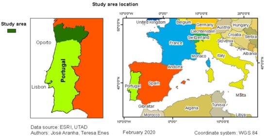
Figure 1.
Study area (North Portugal) and Portugal world geographical location.
This is a very fragmented landscape and the small forest areas are often side by side with shrubland and agricultural areas. It should be noted that, for cultural reasons, the rural population often uses fire as an instrument for pruning as well as a method for removing any residues. The result of this approach is that a higher number of rural fires every year occurs than is actually appropriate for this type of landscape.
The study area in Northern Portugal includes many morphological and edaphoclimatic conditions typical of this region. Altitude ranges from sea level (0 m) to 1546 m in the Gerês mountains (Figure 2). Mean annual accumulated precipitation ranges from 1000 to 2400 mm in the Northwest areas and from 600 to 1200 mm in the Northeast areas. Mean annual temperature ranges from 12.5 °C to 15.0 °C in the Northwest areas and from 7.5 °C to 12.5 °C in the Northeast areas.
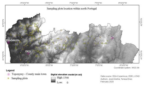
Figure 2.
Sampling plots location.
2.2. Data Sources
2.2.1. Using GIS in the Project
The project aims were to analyse former burnt areas, assess potential vegetation regrowth and to estimate the shrubs’ biomass taking into account the elapsed time since any wildfire took place. The initial process used the burnt areas data. It is possible to download a set of vector files representing the burnt areas’ perimeter by year of occurrence from the Portuguese Forest Services website [35] or the European Forest Fire Information System [36].This information has been used to establish one of the layers within the GIS project since 2000. Every year, the burnt areas’ vector file is updated with new burnt areas boundaries. Spatial analysis then enabled new calculations to be made such as identifying fire recurrence areas as well as assessing the time since the last occurrence of a fire in the same areas.
For the period between 2000 and 2016, 10 sampling plots per year after the last fire were selected. This resulted in 170 sampling points, dispersed throughout North Portugal. In 2017 and 2018, after the severe rural fires that occurred in those years, the GIS project was updated and new sampling plots were added, increasing the number of samples to 234.
These sample points (Figure 2) were then used to create a survey GIS project (e.g., ArcPad, Survey 123, QField) that was transferred to a DGPS receiver (Trimble Inc., Sunnyvale, CA, USA). All the sample points were also marked (based on the GIS layout) on the Topographic Plan of Portugal on a 1/25000 scale. These were then printed to support fieldwork in areas with no GNSS signal.
Thus the data generated from 2000 to 2018 were used to identify the sampling points on the ground enabling us to record any shrub regrowth since the last known fire occurrence.
Circular 500 m2 sampling plots (12.62 m in radius) were used along with the cross transect method. Two 25.24 m fiberglass tape measures were stretched perpendicularly across each sampling plot. Then, the shrubs intersecting each fiberglass tape were measured in 3 dimensions: length, width, and height. This enabled a calculation of the volume, assuming that the shrubs canopy was a sphere, and by using Equation (1).
where Vsh = shrubs canopy volume (m3); L = length (m), W = width (m), H = height (m) (Formula demonstration in Appendix A).
Vsh = 1/6 π L W H
After measuring the total shrubs’ volume along the 2 transects within the sampling plot, 10 shrub plants, 5 per transect (at the edges of the plot, halfway from the center and in the center) were cut in order to be weighed. They were then placed in plastic bags, brought to the lab, put to dry in the shade and weighed after reaching 30% moisture. The achieved results for the 500 m2 circular sampling plots were then extrapolated to an area of 1 hectare and the amount of shrub biomass per plot was estimated using Equation (2).
where Biomass in Mg ha−1, V = total shrubs volume along the 2 transects (m3), W = average shrubs weight (Mg m−3 at 30% moisture), Mxw = maximum width measured along both transects (Formula demonstration in Appendix A).
Biomass = V W 200/Mxw
2.2.2. The Processing and Classification of Sentinel 2 Images
Sentinel 2 images were freely downloaded either from the Copernicus Hub website [37] or from the Glovis website [38].
As the study area is not covered by a single image, eight Sentinel 2 images were used, two per year, for the years of 2016, 2017, 2018, and 2019. All of them were recorded in the summer season.
It was not possible to download Sentinel-2S2A images for the years 2017, 2018 and 2019. Only Sentinel-2L1C were available. When processing these images for the various dates, it was noticed, after computing the NDVI images, that the calculated values for the water surfaces (e.g., dams) were not consistent. This situation led to performing Sentinel-2 SEN2COR280 Processor (7.0.0) analysis by SNAP. For this reason, an images atmospheric calibration was performed, based on the spectral signature of the water collected by the research team with a spectra radiometer Ocean Optics VIS NIR (Spectrecology, Inc., St Petersburg, FL, USA) and on the atmospheric scattered model proposed by Chavez (1988) [39]. This procedure was carried out in order to have the same spectral signature for all water surfaces. Each image was also submitted for atmospheric correction because solar elevation and the state of the atmosphere introduce differences in the radiation detected by the sensor for the same area on different dates [40,41,42,43].
To ensure that differences in reflectance are due to changes in land cover, and not caused by radiometric distortions, it was also necessary to apply a radiometric correction. One of the most used models for atmospheric correction is a process called dark object subtraction (DOS) proposed by reference [39]. This process is based on an atmospheric scattering model and reduces the haze effect by calculating the expected minimum for a given band after atmospheric correction. This was carried out in relation to the following criteria: at-satellite radiances were converted to surface reflectance by correcting for both solar and atmospheric effects. Then, at-satellite radiance values were converted into surface reflectance using a DOS approach [39]. This assumes no atmospheric transmittance loss and no downward diffuse radiation. The surface reflectance of the dark object was assumed to be 1%, and thus the path radiance was assumed to be the dark-object radiance minus the radiance contributed by 1% surface reflectance [39,40,41,42,43].
Spectral reference signatures, such as water, bare soil and dense shrubland, were created after dedicated work using an Ocean Optics VIS NIR spectra radiometer.
After the images processing operations, a RGB false colour composition image and an NDVI image was created for all dates. The Sentinel 2 RGB482 composition was used, because it employs the near infrared band in the green channel which allows the highlighting of vegetation thus enabling an identification of the burnt areas, both recent and old.
Based on the analysis of these new images, and with the support of the GIS project and the orthophotomaps made available by Bing Maps, spectral signatures were created to support the images supervised classification. In a second stage, spectral signatures for the main rural and forest land cover classes were created, namely:
- -
- Agriculture
- -
- Bare soil
- -
- Deciduous
- -
- Burnt areas
- -
- Coniferous
- -
- Grass
- -
- Rocky areas with shrubs
- -
- Shrubs
- -
- Urban areas
- -
- Water
These spectral signatures were then used to perform supervised classification techniques using the 10 m Sentinel 2 bands: B2, B3, B4, and B8. The minimum distance, maximum likelihood, and random forest were tested.
After the supervised classification process completed, a new image was created indicating the burnt areas and shrubland. This is a necessary step whereby a raster mask is created then applied to the NDVI image in order to estimate the shrubs’ biomass that has regrown on former burnt areas.
This raster mask is required because the vector files represent all of the annual burnt areas created. When placed over the relevant satellite images showing the burnt areas boundary or perimeter, they do not consider the unburnt ‘islands’, nor the rocky areas [44,45,46]. Thus, to calculate biomass estimates by means of a vector mask may lead to overestimations. In order to be able to calculate the amount of shrub biomass that regenerated in the former burnt areas, it is necessary to create a raster mask that represents only the areas that were actually burnt.
Finally, the sampling points attribute table in the GIS was updated with the NDVI values using a known technique that enables extracting raster values to point-type vector files. Lastly, this attribute table was exported in dBase format and processed in Excel. This way, it was possible to analyse the relationship that could be established between the measured shrubs’ biomass, and that which was calculated using dedicated field work. In addition an NDVI value was also calculated using satellite images processing techniques.
Figure 3 outlines a summary of all the working stages used in this research.
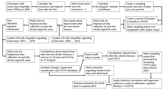
Figure 3.
Work flow chart.
3. Results
3.1. Landcover Characterization
The landcover characterization work carried out was based on false colour RGB482 composition visual analysis (Figure 4) and used NDVI images (Figure 5) for interpretation (all dates). The ensuing results for 2019 are shown in Figure 4 and Figure 5.
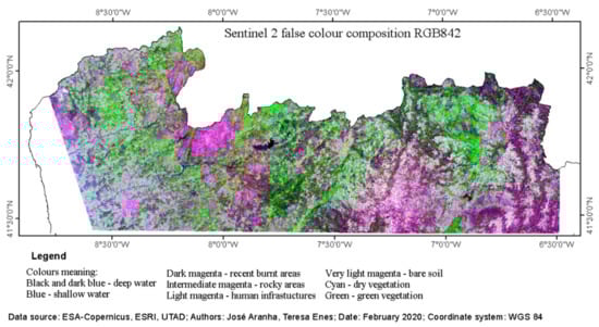
Figure 4.
Sentinel 2 images (summer 2019) for the study area using false colour composition RGB482.
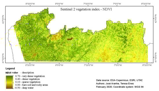
Figure 5.
Sentinel 2 images (summer 2019) for the study area using an NDVI calculation.
As healthy vegetation has its maximum spectral reflectance in near-infrared wavelength, the Sentinel 2 band 8 (near-infrared) was used and coloured in green. Thus, green tonalities depicted in the RGB482 images indicated vegetation density and consequently the darker the green colour indicated the denser the vegetation.
The vegetation index NDVI was calculated using the normalized difference between the near-infrared and the red images. As the vegetation red reflectance is always lower to the near-infrared reflectance, the positive NDVI achieved values could also indicate vegetation density. Thus, the higher the NDVI values the denser the vegetation. Each of the dots depicted in Figure 2 represent a sampling point within a former burnt area. Analysing the NDVI image, Figure 5, it appears that the old burnt areas are in various states of vegetation recovery. It seems, therefore, that the Northwest area of Portugal has more dense vegetation and less burnt areas scars than the Northeast area.
It appears, however, that neither the green colour intensity shown in the RGB482 images (Figure 4) nor the NDVI values (Figure 5) enable a classification of the vegetation type (e.g., burnt areas, forest land, shrubland). These two images alone only infer the potential density of the vegetation cover. Thus, it was necessary to carry out further analysis using Sentinel 2 images and an assisted classification process to classify the land cover in classes.
Using the results from the Sentinel 2 images supervised classification process as well as the Minimum Distance Classifier, enabled us to state that the main land cover features are suitable to be classified accurately as presented in Table 2. This classification accuracy is particularly high for forest features. For example, burnt areas and shrubland was easy to identify and classify with an accuracy over 80%.
Table 2.
Achieved results after confusion matrix for classification accuracy from Sentinel-2 images.
It was possible, therefore, to create a mask image for use with an associated NDVI image in order to isolate burnt areas and shrubland. This mask was later used to ‘cut’ the NDVI image enabling a shrub biomass calculation to be carried out along with the allometric equation application.
With an overall accuracy of 79.6% and a Cohen’s K coefficient of 0.754, it can be stated that the Sentinel 2 images were found to be suitable for use in forestry applications as well as in the dynamic analysis of former burnt areas too. The Sentinel 2 classified images created a raster mask that was used subsequently to isolate the burnt areas and the shrubs areas.
3.2. Allometric Model for Shrub Biomass Estimation
For the allometric equation adjustment, 110 pairs (NDVI, shrub biomass) were used: 46 extracted from 2016 image, 33 from 2017 image and 31 from 2018 image. In a first approach to data processing, descriptive statistics were calculated for each date and region, as presented in Table 3.
Table 3.
Descriptive statistic for the sub-samples.
Subsequently, student-t tests were performed in order to verify that the sample points for the NW area of Portugal are different to those of the sample points for the NE area. As no significant differences were found, all the sampling points for each year were then merged into a single sample file.
The NDVI and shrub biomass values were centered and reduced in order to verify if this composite sample had a normal distribution. Descriptive statistic and accumulated probability values were calculated. Initially, the descriptive statistic for NDVI and shrubs biomass was calculated, shown in Table 4. Then, accumulated probability values were calculated as depicted in Figure 6.
Table 4.
Descriptive statistic for the total sample.
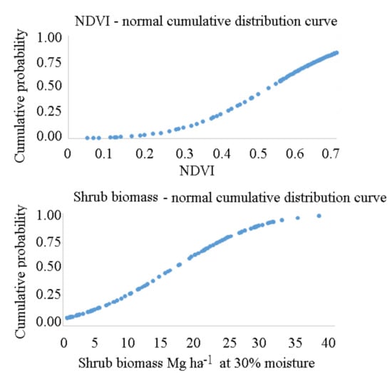
Figure 6.
Normal cumulative curves to NDVI (top) and to shrubs biomass (bottom).
The achieved results show that both distributions presented a normal distribution (Figure 6).
In the third stage of the process, a XY graphical representation was used in order to analyse the relationship that could be established between NDVI values and shrub biomass (Figure 7). The resulting graphic shows a narrow points cloud on the left for the minimum values and a scattered cloud on the right for the maximum values. This indicates that there were constraints in the regression analysis for the allometric equation calculation, possibly suggesting that there were too few options available.
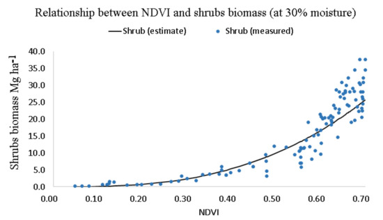
Figure 7.
Relationship between NDVI and shrub biomass.
During the regression analysis processing, it was noted that the NDVI tends to saturate at 0.7, suggesting that the shrubs’ growth process maybe asymptotic to approximately 50 Mg ha−1. This maybe due to the nature of the plants and the space they occupy over periods of time. As a consequence of the approach adopted, the ensuing model led to better results than anticipated. It is presented in Equation (3).
R2 = 0.8984 (p-value < 0.05) and RMSE = 4.46 Mg ha−1
Shrub biomass = 70.078 NDVI 2.8113
3.3. Shrub Biomass Estimation Using NDVI Image Processing
When the regression analysis completed, the adjusted allometric equation was used to generate the shrubs’ biomass estimation using the NDVI. It was also applied to the 2019 Sentinel 2 images before the final calculation. General NDVI images were submitted to mask extraction in order to create new images indicating the former burnt and shrub areas, as depicted in Figure 8.
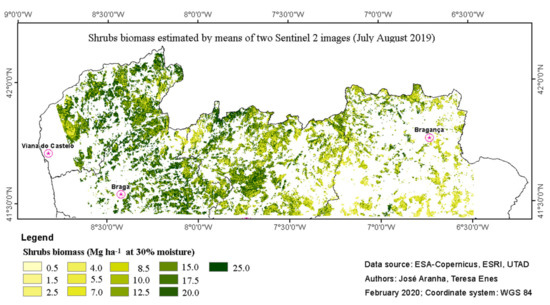
Figure 8.
Accumulated shrubs’ biomass in former burnt areas in the North of Portugal, estimated using an NDVI image summer 2019 and an allometric equation.
The results show that it is possible to account for an extent of some 172,022 ha and of 1,323,222 Mg of accumulated shrubs’ biomass in the Northeast area. Likewise some 209,824 ha and 3,835,047 Mg can be identified in the Northwest area. On average, the Northeast area has approximately 7.7 Mg ha−1 and the Northwest has 18.3 Mg ha−1 of accumulated shrubs’ biomass identified in the former burnt areas and shrubland.
4. Discussion
4.1. Sentinel 2 Images
The Sentinel 2 images, bands B2, B3, B4 and B8 (VIS–NIR), were deemed to be suitable for use in rural areas characterization and mapping, mainly in forested and shrubland areas, as demonstrated by the calculated overall accuracy (OA = 79.6) and the Cohen’s K coefficient (k = 0.754) described earlier.
It was possible to classify, with good accuracy, the forest features in deciduous, coniferous and shrubs areas too. It was not possible, however, to classify mixed forest stands of deciduous and coniferous woodlands as the classification methods only isolate deciduous clusters from coniferous clusters. It was also not possible to classify forest stands by species.
Due to their spectral signatures, burnt areas were identified and classified with an users’ accuracy of 89%. It was only possible to classify these former burnt areas, i.e., younger than a year and a half, after the fire because this timeframe indicates when a vegetative period has taken place and the shrubs were beginning to grow in these burnt areas. For example, if two full years have passed since the fire, the former burnt areas classification through satellite images starts to present results that confuse these areas with agricultural land and rocky areas with scattered vegetation.
The B4 and B8 bands enabled us to calculate NDVI images which proved to be adequate for the shrubs’ biomass characterization and quantification. This was demonstrated using the statistical values of correlation between NDVI and shrubs biomass (r = 0.853) and the determination coefficient for the allometric equation (R2 = 0.8984).
4.2. Shrubland Characterization
Vegetation, mainly shrubs, has a great potential to regrow on former burnt areas. The capability to colonize the space and to produce biomass is closely related to local morphology and edaphoclimatic conditions. As previously presented in Table 3, after calculating descriptive statistics for sub-samples and after adjusting allometric equations to each year, no statistically significant differences were found. In order to guarantee the accuracy of the estimates obtained by the general allometric equation now presented, however, it is necessary to verify if the growth rate of the shrubs is different in the two study areas. To achieve this, an allometric equation per area to the pairs was developed using: age and shrubs’ biomass. This is presented as Equations (4) and (5).
R2 = 0.7349 (p-value < 0.05) and RMSE = 4.9 Mg ha−1
R2 = 0.6921 (p-value < 0.05) and RMSE = 3.7 Mg ha−1
NW region: Shrub biomass = −0.0062 t3 + 0.2089 t2 − 0.2738 t + 2.279
NE region: Shrub biomass = −0.0072 t3 + 0.2211 t2 − 0.2738 t + 2.043
The resulting shrubs’ estimates, by means of these two equations, showed that there was no statistically significant differences found between regrowth rate in either of the study areas. This is shown in Figure 9.
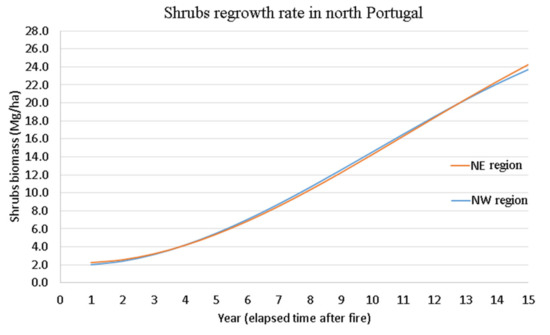
Figure 9.
Estimations for shrubs regrowth rates in the study area.
The Northwest study area was found to have better morphological and edaphoclimatic conditions for shrubs’ regrowth after fire than the Northeast area, possibly because the latter had retained burnt area scars for a longer time. After 30 years of forest fires, many of the mountainous areas had lost almost all vegetation and, as a consequence, top soil too. Figure 4 and Figure 5 show that these areas are now characterized by small forested spaces or shrub zones surrounded by rocky extents with scattered shrubs.
The achieved results were classified regarding the average value of accumulate shrubs’ biomass according to the elapsed time after the last fire event and the sampling date. This reclassification process enabled us to calculate the accumulated shrubs’ biomass amount per class and also to create a histogram for the number of available hectares per class. The results are shown in Figure 10.
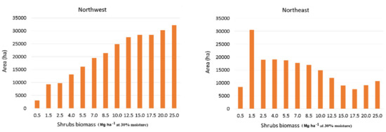
Figure 10.
Accumulated shrubs biomass in summer 2019.
Although the growth rates in the two areas are not significantly different, it appears that the Northwest area is more densely vegetated than the Northeast. This was expected since this former area is facing the Atlantic Ocean, has a milder climate and greater rainfall than the Northeast landlocked territory.
It can be noted that for both of the study areas, within two years, the vegetation was capable to regrow enough to disguise the black landscape caused by fire. After five years, almost all the former burnt area was covered by vegetation and the accumulated shrubs’ biomass grew up to 5 Mg ha−1 (30% moisture). Thus it can be demonstrated that in up to five years after a fire occurrence, the ecosystem will recover as evidenced by the fire hard index ranges from very low to medium. It appears that between five and 10 years after a fire, the accumulated shrubs’ biomass can reach 14 to 18 Mg ha−1. In terms of the ecosystem, the situation is favorable, but in terms of fire danger less so. Between 10 and 15 years after a fire, the shrubs’ accumulated biomass can reach 26 Mg ha−1. It must be noted, however, that this biomass already has a large wood structure that gives it properties suitable for its use as fuel for thermoelectric power plants. This means that this shrubs biomass has a potential economic value that could change very dense shrubs areas from a severe fire hazard issue into a green fuel source.
4.3. Allometric Equation for Shrub Biomass Estimation
The accumulated shrubs’ biomass estimation was made using an allometric equation based on the elapsed time after a fire, as previously presented in Section 4.2 and also shown in Equations (4) and (5) as well as Figure 9. In addition the NDVI values derived from satellite image processing, also played a significant role (described earlier in this paper).
When working in a large area that presents different morphological and edaphoclimatic characteristics and which requires the use of multiple satellite scenes, it is appropriate to verify in advance if there are differences in the shrubs’ growth rate and if there are differences in relation to the year under study. It was verified, as previously stated, that no statistically significant differences were found in relation to the shrubs’ growth rate of the bush in the two study areas.
To verify the second hypothesis, an allometric equation for each date was adjusted. This is presented in Table 5.
Table 5.
Allometric equations adjusted for the 3 years in analysis.
Each of the allometric equations used the 110 sampling points and consequently the results generated were very similar with no significant differences found between estimates. These are shown in Figure 11.
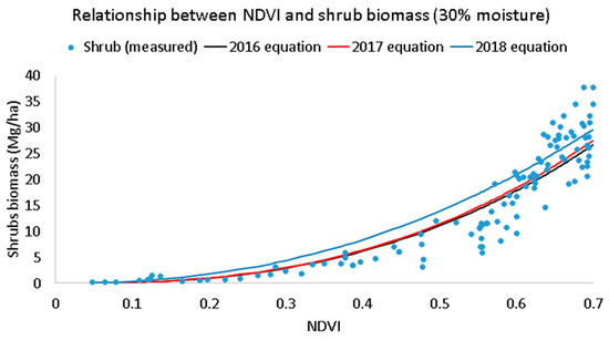
Figure 11.
Relationship between NDVI and shrubs biomass estimates.
As no statistically significant differences were found between the shrubs’ biomass estimations using the three previously presented equations, a general equation was developed using the 110 sampling points (Equation (3)).
The adjusted allometric equation described here proved to be suitable for assessing the shrubs’ biomass estimation using NDVI values. Employing this method also made it possible to monitor the shrubs’ biomass regrowth in the former burnt areas on a regular basis by means of Sentinel 2 image processing and classification.
As neither the shrubs’ growth rates are significantly different for either study area or the use of the allometric equations (adjusted for each of the years: 2016, 2017, and 2018) led to statistically significant estimates between them and to the general equation, it can be state that the methodology was suitable to be used in this area for any year. This has been demonstrated by using accurate estimates of the accumulated shrubs’ biomass (based on satellite imagery) and on a regular basis. It also enables the monitoring of the shrubs’ biomass variation as well as calculating the biomass gains and losses. Biomass gains can be converted into sequestered carbon and used to analyse the ecosystem’s state of health as well as its production capability [47,48]. It can also be used to update the fire hazard indices calculation and to identify the places most prone to be burnt by large fires and, therefore, requiring special attention. Biomass losses can be converted into carbon released into the atmosphere by forest fires [9] or used to calculate the intensity of forest fires. The difference between post-fire gains and losses can be used to calculate the fire severity [46,49] in any given spot.
This equation was adjusted for the North Portugal study areas and it is suggested that it could be used in other territories with similar morphological and edaphoclimatic conditions. It is important to remember, however, that such work requires a validation process for any area.
5. Conclusions
Free Sentinel 2 images were an asset to derive multi temporal and dynamic studies about land cover, for monitoring former burnt areas and to estimate the shrubs’ biomass accumulation.
The achieved results enable us to state that the methodology presented in this manuscript proved to be robust and that the NDVI derived from Sentinel 2 images can be used to calculate accurate and dynamic estimates of accumulated shrubs biomass.
The allometric equation presented here also allowed us to estimate the shrubs’ biomass using Sentinel 2 images without depending on the vector files provided by EFFIS or by ICNF (Portuguese Institute for Nature and Forest). Comparing the shrubs’ biomass estimates achieved through the two allometric equations, using NDVI and using elapsed time after fire, demonstrated that no statistically significant differences were found. Thus, it can be stated that the allometric equation presented in this manuscript incorporated the effect of elapsed time after the fire.
The combined use of GIS and RS techniques, complemented by regression analysis proved to be useful for monitoring the shrubs’ regrowth in the former burnt areas. It was also useful to analyse the land cover dynamics and also to quantify the accumulated shrubs’ biomass. GIS supported data records, management, and the sampling system development was helpful whilst RS supported multitemporal land cover analysis and biomass estimation using associated satellite image processing. Classification also offered major benefits too.
Regression analysis and allometric equation adjustments were found to be suitable processes to assign the biophysical data that was collected via field work as well as the use of the freely available satellite images. This led to the calculation and estimatation of the shrubs’ biomass.
Although the NDVI saturates only measured 0.7, it was still possible to obtain good estimates of the shrubs’ biomass before the complete canopy closure which is when the accumulated values reach their maximum. It was discovered that the NDVI values were not, however, specific for all types of vegetation. Consequently it was always necessary to create a raster mask in advance that identified the type of vegetation or area under analysis in order to define the estimates for those particular places of interest.
From a forest management perspective, it was found that, after five years, the accumulated shrubs’ biomass starts to be a fire hazard related issue as it creates a horizontal continuous coverture which encourages any fire to spread. If it was 10 years since the last fire occurrence, the amount of accumulated shrubs’ biomass was found to be over 14 Mg ha−1 which led to a severe wild fires spread. This is commonly referred to as a 10 year of fire recurrence cycle in Portugal.
The methodology presented in this paper was found to be suitable for use in forest land management and also served a number of unexpected different purposes. From an ecological persepective it has been demonstrated that, over a two-year period, the vegetation was capable of enough regrowth to minimize erosion actions and to support animal life. In a five-year period, it appears that almost all the former burnt areas are covered by vegetation. From this point of view it may be possible to use the shrubs’ biomass for energy purposes but it was found that only after a 10-year period that the amount of accumulated shrubs’ biomass became economically valuable to cut and transport elsewhere. This was determined by the monetary biomass value for any potential power plant location, the man hours cost involved to capture it as well as the necessary transportation costs.
Author Contributions
Conceptualization, J.A.; performed the experiment and analysis, J.A., T.E., H.V. and A.C.; performed the statistical analysis, J.A., T.E., A.C. and H.V.; resources, H.V., A.C. and J.A.; writing—original draft preparation, T.E., J.A.; writing—review and editing, J.A., H.V.; project administration, J.A. All authors have read and agreed to the published version of the manuscript.
Funding
This research is supported by National Funds by FCT—Portuguese Foundation for Science and Technology, under the project UIDB/04033/2020.
Acknowledgments
The authors would like to express their sincere thanks for the critical review of the manuscript carried out by Teresa Connolly.
Conflicts of Interest
The authors declare no conflict of interest.
Appendix A
Additional information:
- Sentinel-2S2A_20160828T113040_20160828T164718_A006183_T29TPG_N02_04_01
- Sentinel-2S2A_20150804T113226_20160319T010337_A000606_T29TPN_N02_04_01
- Sentinel-2L1C_T29TPG_A010759_20170714T112114
- Sentinel-2L1C_T29TNG_A010759_20170714T112114
- Sentinel-2L1C_T29TPG_A015621_20180619T112602
- Sentinel-2L1C_T29TNG_A006784_20180624T112452
- Sentinel-2L1C_T29TNG_A021341_20190724T112448
- Sentinel-2L1C_T29TPG_A021484_20190803T112140
Formulae demonstration:
where Vsh = shrubs canopy volume (m3), L = length (m), W = width (m), H = height (m), and the volume of a sphere = 4/3 π r3.
Vsh = 1/6 π L W H
In order to use the shrubs dimensions measured along the transect, the equation can be rewritten as:
where Biomass in Mg/ha V = Total shrubs volume along the 2 transects (m3) W = Average shrubs weight (Mg/m3 at 30% moisture) Mxw = Maximum width measured along both transects.
Volume of shrub canopy= 4/3 π Length/2 Width/2 Height/2
Volume of shrub canopy= 4/24 π Length Width Height
Volume of shrub canopy= 1/6 π Length Width Height
Biomass = V W 200/Mxw
In a 500 m2 sampling plot, the plot radius is 12.62 m. This way, each transect has 25.24 m. The 2 transect account for 50.48 m.
When measuring the shrubs along these transects, the sum of shrubs width plus shrubs length define the area occupied by shrubs within the 2 cross section transects. Using the maximum measured shrubs width and the length of both transects is possible to calculate the maximum area for the 2 transects.
Sampling area = Maximum width 50.48 m
For converting the measured shrubs biomass within the sampling area, it is necessary to convert this area to 1 hectare.
10,000/Maximum width 50.48 ≈ 200/Maximum width
References
- Caetano, M.; Igreja, C.; Marcelino, F.; Costa, H. Estatísticas e dinâmicas territoriais multiescala de Portugal Continental 1995–2007–2010 com base na Carta de Uso e Ocupação do Solo (COS). Direcção Geral do Território 2017, 149. [Google Scholar]
- Oliveira, S.L.J.; Pereira, J.M.C.; Carreiras, J.M.B. Fire frequency analysis in Portugal (1975–2005), using Landsat-based burnt area maps. Int. J. Wildl. Fire 2011, 21, 48–60. [Google Scholar] [CrossRef]
- Marques, S.; Borges, J.G.; Garcia-Gonzalo, J.; Moreira, F.; Carreiras, J.M.B.; Oliveira, M.M.; Cantarinha, A.; Botequim, B.; Pereira, J.M.C. Characterization of wildfires in Portugal. Eur. J. For. Res. 2011, 130, 775–784. [Google Scholar] [CrossRef]
- Parente, J.; Pereira, M.G.; Amraoui, M.; Tedim, F. Science of the Total Environment Negligent and intentional fires in Portugal: Spatial distribution characterization. Sci. Total Environ. 2018, 624, 424–437. [Google Scholar] [CrossRef] [PubMed]
- Pereira, M.G.; Aranha, J.; Amraoui, M. Land cover fire proneness in Europe. For. Syst. 2014, 23, 598–610. [Google Scholar] [CrossRef]
- Ferreira Leite, F.; Bento Gonçalves, A.; Vieira, A. The recurrence interval of forest fires in Cabeço da Vaca (Cabreira Mountain-northwest of Portugal). Environ. Res. 2011, 111, 215–221. [Google Scholar] [CrossRef] [PubMed]
- Ursino, N.; Romano, N. Wild forest fire regime following land abandonment in the Mediterranean region. Geophys. Res. Lett. 2014, 41, 8359–8368. [Google Scholar] [CrossRef]
- Cerdá, A.; Doerr, S.H. Influence of vegetation recovery on soil hydrology and erodibility following fire: An 11-year investigation. Int. J. Wildl. Fire 2005, 14, 423–437. [Google Scholar] [CrossRef]
- Pereira da Silva, T.; Cardoso Pereira, J.M.; Paúl, P.J.C.; Teresa Santos, M.N.; José Vasconcelos, M.P.; de Investigação, B.; Catedrático, P.; Auxiliar, I. Estimativa de Emissões Atmosféricas Originadas por Fogos Rurais em Portugal Estimate of Atmospheric Emissions Originated by Wildfires in Portugal. Silva Lusit. 2006, 14, 239–263. [Google Scholar]
- Viana, H. Modelling and Mapping Aboveground Biomass for energy Usage and Carbon Storage Assessment in Mediterranean Ecosystems. Ph.D. Thesis, Universidade de Trás os Montes e Alto Douro, Vila Real, Portugal, 2012. [Google Scholar]
- Aranha, J.; Calvão, A.R.; Lopes, D.; Viana, H. Quantificação Da Biomassa Consumida Nos Últimos 20 Anos De Fogos Florestais No Norte Portugal. Info 2011, 26, 44–49. [Google Scholar]
- Kazanis, D.; Xanthopoulos, G.; Arianoutsou, M. Understorey fuel load estimation along two post-fire chronosequences of Pinus halepensis Mill. forests in Central Greece. J. For. Res. 2012, 17, 105–109. [Google Scholar] [CrossRef]
- DL 76/2017-5.ª alteração ao DL 124-2006. Diário da República n.º 158/2017, Série I de 2017-08-17. DR. J. Portuguese Rep. 2017, 4734–4762. [Google Scholar]
- Viana, H.; Fernandes, P.; Rocha, R.; Lopes, D.; Aranha, J. Alometria, Dinâmicas da Biomassa e do Carbono Fixado em Algumas Espécies Arbustivas de Portugal. 6.º Congr. Florest. Nac. 2009, 244–252. [Google Scholar]
- Gratani, L.; Varone, L.; Ricotta, C.; Catoni, R. Mediterranean shrublands carbon sequestration: Environmental and economic benefits. Mitig. Adapt. Strateg. Glob. Chang. 2013, 18, 1167–1182. [Google Scholar] [CrossRef]
- Cairns, M.A.; Lajtha, K.; Beedlow, P.A. Dissolved carbon and nitrogen losses from forests of the Oregon Cascades over a successional gradient. Plant Soil 2009, 318, 185–196. [Google Scholar] [CrossRef]
- Zuazo, V.H.D.; Pleguezuelo, C.R.R. Soil-erosion and runoff prevention by plant covers: A review. Agron. Sustain. Dev. 2008, 28, 65–86. [Google Scholar] [CrossRef]
- Imeson, A. Desertification, Land Degradation and Sustainability; John Wiley & Sons: West Sussex, UK, 2012; ISBN 1119978483. [Google Scholar]
- Bochet, E.; Poesen, J.; Rubio, J.L. Runoff and soil loss under individual plants of a semi-arid Mediterranean shrubland: Influence of plant morphology and rainfall intensity. Earth Surf. Process. Landforms 2006, 31, 536–549. [Google Scholar] [CrossRef]
- Mangas, J.G.; Lozano, J.; Cabezas-Díaz, S.; Virgós, E. The priority value of scrubland habitats for carnivore conservation in Mediterranean ecosystems. Biodivers. Conserv. 2008, 17, 43–51. [Google Scholar] [CrossRef]
- Sandifer, P.A.; Sutton-Grier, A.E.; Ward, B.P. Exploring connections among nature, biodiversity, ecosystem services, and human health and well-being: Opportunities to enhance health and biodiversity conservation. Ecosyst. Serv. 2015, 12, 1–15. [Google Scholar] [CrossRef]
- Helming, K.; Diehl, K.; Geneletti, D.; Wiggering, H. Mainstreaming ecosystem services in European policy impact assessment. Environ. Impact Assess. Rev. 2013, 40, 82–87. [Google Scholar] [CrossRef]
- Viana, H.; Cohen, W.B.; Lopes, D.; Aranha, J. Assessment of forest biomass for use as energy. GIS-based analysis of geographical availability and locations of wood-fired power plants in Portugal. Appl. Energy 2010, 87, 2551–2560. [Google Scholar] [CrossRef]
- Quinta-Nova, L.; Fernandez, P.; Pedro, N. GIS-Based Suitability Model for Assessment of Forest Biomass Energy Potential in a Region of Portugal. IOP Conf. Ser. Earth Environ. Sci. 2017, 95, 042059. [Google Scholar] [CrossRef]
- Cohen, W.B.; Maiersperger, T.K.; Spies, T.A.; Oetter, D.R. Modelling forest cover attributes as continuous variables in a regional context with Thematic Mapper data. Int. J. Remote Sens. 2001, 22, 2279–2310. [Google Scholar] [CrossRef]
- Botequim, B.; Zubizarreta-Gerendiain, A.; Garcia-Gonzalo, J.; Silva, A.; Marques, S.; Fernandes, P.M.; Pereira, J.M.C.; Tomé, M. A model of shrub biomass accumulation as a tool to support management of portuguese forests. iForest 2014, 8, 114–125. [Google Scholar] [CrossRef]
- Nguyen, H.K.L.; Nguyen, B.N. Mapping biomass and carbon stock of forest by remote sensing and GIS technology at Bach Ma National Park, Thua Thien Hue province. J. Viet. Env. 2016, 8, 80–87. [Google Scholar]
- Deng, S.; Shi, Y.; Jin, Y.; Wang, L. A GIS-based approach for quantifying and mapping carbon sink and stock values of forest ecosystem: A case study. Energy Proc. 2011, 5, 1535–1545. [Google Scholar] [CrossRef]
- Wijaya, A.; Kusnadi, S.; Gloaguen, R.; Heilmeier, H. Improved strategy for estimating stem volume and forest biomass using moderate resolution remote sensing data and GIS. J. For. Res. 2010, 21, 1–12. [Google Scholar] [CrossRef]
- Roy, P.S.; Ravan, S.A. Biomass estimation using satellite remote sensing data—An investigation on possible approaches for natural forest. J. Biosci. 1996, 21, 535–561. [Google Scholar] [CrossRef]
- Chen, W.; Zhao, J.; Cao, C.; Tian, H. Shrub biomass estimation in semi-arid sandland ecosystem based on remote sensing technology. Glob. Ecol. Conserv. 2018, 16, e00479. [Google Scholar] [CrossRef]
- Norovsuren, B.; Tseveen, B.; Batomunkuev, V. Estimation for Forest Biomass and Coverage Using Satellite Data in Small Scale Area, Mongolia. IOP Conf. Ser. Eart Environ. Sci. 2019, 320, 012019. [Google Scholar] [CrossRef]
- Filella, I.; Peñuelas, J.; Llorens, L.; Estiarte, M. Reflectance assessment of seasonal and annual changes in biomass and CO2 uptake of a Mediterranean shrubland submitted to experimental warming and drought. Remote Sens. Environ. 2004, 90, 308–318. [Google Scholar] [CrossRef]
- Xiao, J.; Moody, A. A comparison of methods for estimating fractional green vegetation cover within a desert-to-upland transition zone in central New Mexico, USA. Remote Sens. Environ. 2005, 98, 237–250. [Google Scholar] [CrossRef]
- ICNF. Available online: http://www2.icnf.pt/portal/florestas/dfci/inc (accessed on 8 January 2020).
- EFFIS. Available online: https://effis.jrc.ec.europa.eu/applications/data-request-form (accessed on 8 January 2020).
- Copernicus. Available online: https://scihub.copernicus.eu/dhus/#/home (accessed on 10 January 2020).
- Glovis. Available online: https://glovis.usgs.gov/app (accessed on 10 January 2020).
- Chavez, P.S. An improved dark-object subtraction technique for atmospheric scattering correction of multispectral data An Improved Dark-Object Subtraction Technique for Atmospheric Scattering Correction of Multispectral Data. Remote Sens. Environ. 1988, 24, 459–479. [Google Scholar] [CrossRef]
- Teillet, P.M.; Staenz, K.; William, D.J. Effects of spectral, spatial, and radiometric characteristics on remote sensing vegetation indices of forested regions. Remote Sens. Environ. 1997, 61, 139–149. [Google Scholar] [CrossRef]
- Louis, J.; Debaecker, V.; Pflug, B.; Main-knorn, M.; Bieniarz, J. Sentinel-2 Sen2cor: L2a Processor for Users. In Proceedings of the Living Planet Symposium, Prague, Czech Republic, 9–13 May 2016; Volume 2016, pp. 9–13. [Google Scholar]
- Sola, I.; García-Martín, A.; Sandonís-Pozo, L.; Álvarez-Mozos, J.; Pérez-Cabello, F.; González-Audícana, M.; Llovería, R. Montorio Assessment of atmospheric correction methods for Sentinel-2 images in Mediterranean landscapes. Int. J. Appl. Earth Obs. Geoinf. 2018, 73, 63–76. [Google Scholar] [CrossRef]
- Sentinel Online. Available online: https://sentinel.esa.int/web/sentinel/user-guides/sentinel-2-msi/processing-levels/level-2 (accessed on 9 January 2020).
- Meddens, A.J.H.; Kolden, C.A.; Lutz, J.A.; Abatzoglou, J.T.; Hudak, A.T. Spatiotemporal patterns of unburned areas within fire perimeters in the northwestern United States from 1984 to 2014. Ecosphere 2018, 9, 1–16. [Google Scholar] [CrossRef]
- Tedim, F.; Royé, D.; Bouillon, C.; Fernando, J.M.C.; Leone, V. Understanding unburned patches patterns in extreme wildfire events: A new approach. In Proceedings of the Advances in forest fire research—VIII International Conference on Forest Fire Research, Coimbra, Portugal, 9–16 November 2018; Viegas, D.X., Ed.; pp. 700–715. [Google Scholar] [CrossRef]
- Picos, J.; Alonso, L.; Bastos, G.; Armesto, J. Event-based integrated assessment of environmental variables and wildfire severity through Sentinel-2 Data. Forests 2019, 10, 1021. [Google Scholar] [CrossRef]
- Iqbal, K.; Hussain, A.; Negi, A.K. An overview of Biomass Estimation methods. Res. J. Soc. Sci. Manag. 2014, 4, 42–57. [Google Scholar]
- Banti, M.A.; Kiachidis, K.; Gemitzi, A. Estimation of spatio-temporal vegetation trends in different land use environments across Greece. J. Land Use Sci. 2019, 14, 21–36. [Google Scholar] [CrossRef]
- Díaz-Delgado, R.; Lloret, F.; Pons, X. Influence of fire severity on plant regeneration by means of remote sensing imagery. Int. J. Remote Sens. 2003, 24, 1751–1763. [Google Scholar] [CrossRef]
© 2020 by the authors. Licensee MDPI, Basel, Switzerland. This article is an open access article distributed under the terms and conditions of the Creative Commons Attribution (CC BY) license (http://creativecommons.org/licenses/by/4.0/).