Article

Forest Landscape Heterogeneity Increases Shrub Diversity at the Expense of Tree Seedling Diversity in Temperate Mixedwood Forests

by
Rudiger Markgraf
1,
Frédérik Doyon
2,3,* and
Daniel Kneeshaw
1
1
Centre d’étude de la Forêt, Département des Sciences Biologiques, Université du Québec à Montréal, 141 Avenue du Président-Kennedy, Montréal, QC H2X 1Y4, Canada
2
Département des Sciences Naturelles, Université du Québec en Outaouais, 283 Boulevard Alexandre-Taché, Gatineau, QC J8X 3X7, Canada
3
Institut des Sciences de la Forêt Tempérée, 58 rue Principale, Ripon, QC J0V 1V0, Canada
*
Author to whom correspondence should be addressed.
Forests 2020, 11(2), 160; https://doi.org/10.3390/f11020160
Submission received: 10 December 2019 / Revised: 23 January 2020 / Accepted: 29 January 2020 / Published: 31 January 2020
(This article belongs to the Special Issue Role of Gap Factors in Forest Tree Regeneration and Plant Communities)

Abstract

:
Partial disturbances enhance spatial heterogeneity through the diversification of forest structure, which contributes to niche partitioning and consequently to species diversity. However, this heterogeneity–diversity relationship may differ between groups of species, and is potentially modified by biotic interactions at the community level. We propose that shrub diversity will be greater in heterogeneous landscapes, while tree diversity will be lower in those same landscapes, due to the biotic interactions of shrub competition. We conducted field sampling in the balsam fir/yellow birch bioclimatic domain in western Québec, a forested ecosystem disturbed by natural and anthropogenic partial disturbances. We selected 12 forested landscapes (1 km2), four in each of three classes of landscape heterogeneity (heterogeneous, moderately heterogeneous, homogenous). Shrub and tree species regeneration abundance was measured in three different size classes of canopy gaps and the forest understory. Gap proportions were assessed in each landscape using aerial LiDAR data. Tree and shrub alpha-diversity significantly responded to landscape heterogeneity, shrubs being more diverse while tree seedlings were less diverse in heterogeneous landscapes. Heterogeneous landscapes showed highest species accumulation rates for shrubs in medium-sized gaps. For tree seedlings, species accumulation rates were highest in heterogeneous landscapes in the forest understory. Our study thus supports the heterogeneity–diversity relationship with shrubs having higher alpha and beta diversity in heterogeneous landscapes whereas local-scale tree diversity was higher in homogenous landscapes.

1. Introduction

Species diversity is influenced differently by environmental heterogeneity acting across multiple scales [1]. A hierarchical approach to understanding the patterns of biodiversity includes consideration of the roles of factors that act as filters to species coexistence at different spatial and temporal scales [2,3]. At the site scale, both biotic and abiotic conditions determine habitat quality and temporal variation, which influences local species persistence. At the landscape scale, environmental heterogeneity in abiotic conditions provides the underlying fabric over which different ecosystem trajectories are manifested, generating a mosaic of community assemblages that shift due to landscape disturbance regimes and succession [4,5]. Indeed, the mortality of individuals and groups of trees due to various disturbances, be they natural, such as windfall, insect outbreaks or tree senescence, or anthropogenic (partial harvesting), creates canopy openings of various sizes that persist for different lengths of time. Tree mortality continuously reshapes forest structure at different scales, thus contributing to spatiotemporal heterogeneity in resources.
Heterogeneous landscapes have a greater number and/or variability of habitat types (landscape composition) and a more complex heterogeneous spatial pattern of habitat patches (landscape configuration) [6]. The surrounding habitat patches can influence the regional species pool, species dispersal, biotic competitive interactions, ecosystem function and select for species traits [6,7,8,9]. Mechanisms for positive influence of landscape heterogeneity on diversity include (1) a greater number of species associated with different habitats, (2) species that depend on a variety of patches at different stages of their life-history and (3) reduced dispersal between patches of the same type due to a greater diversity of cover types and therefore a lower proportion of each cover type in the landscape, thus reducing the successful dispersal of potentially competitive species and favouring coexistence [6]. Alternatively, heterogeneity producing smaller habitat patches may positively influence dispersal-limited species across all cover types, and therefore richness due to smaller dispersal distances between smaller patches and diffusion of propagule sources from surrounding species into disturbed areas [10]. Mass effects describe plant species immigration from neighbouring patches into less favourable habitats [11,12,13], while other potential mechanisms include heterogeneous landscapes that maintain a varied seed source due to neighbourhood effects [14,15].
In balsam fir/yellow birch (bF/yB) forests, competitive shrubs exhibit traits more adapted to an increase in disturbance frequency, such as persistence in low resource conditions, resistance to disturbances and fast vegetative growth for rapid colonization of newly created habitat patches [16]. Shrubs take advantage of heterogeneous forest light environments using high trait plasticity to quickly adapt to changing conditions [17]. Therefore, in a shifting landscape mosaic with greater spatiotemporal environmental heterogeneity, we can expect to observe greater shrub diversity both locally and across sites [3,18,19,20].
Local biodiversity may be influenced by immigration, emigration, competitive exclusion or extinction [11]. Therefore, heterogeneity–diversity relationships (HDR) can be masked by community-level biotic interactions. Competition is thus expected to reduce diversity as a small number of species dominate [21]. In bF/yB forests, the greater colonizing and persisting traits of shrubs suggests that this taxonomic group may be able to limit tree regeneration at the landscape scale through greater regional seed pools and due to an increase in the frequency and the recurrence of intermediate disturbances [22,23]. Indeed, Royo and Carson [24] noted a worldwide phenomenon of tree regeneration recruitment failing in forest understories due to an increase in competitive shrubs and herb understory layers (which they called “recalcitrant understory layers”). Trees would thus be relegated to more homogenous and predictable environments where their longevity dominance traits would permit them to dominate both regionally and locally [25].
The objective of this study was to verify whether HDR had consistent effects on two species groups, shrubs and tree seedlings, given the potential biotic interaction between these two groups. We expected that shrub diversity would be greater in heterogeneous landscapes, while tree diversity would be lower in those same landscapes, due to shrub competition. More specifically, we expected (1) that local (alpha-diversity) shrub diversity would be greatest in heterogeneous landscapes while tree regeneration alpha-diversity would be lower in heterogeneous landscapes. We also expected (2) that gaps, due to greater resource availability and local micro-heterogeneity, should be characterised by greater alpha-diversity for both shrubs and tree regeneration when compared to forest understories, with the greatest diversity occurring in the larger gaps [26,27,28,29]. Our third (3) hypothesis stipulated that heterogeneous landscapes should have greater species turnover rate (beta-diversity) for shrubs [12,30,31], but not for tree regeneration, mostly because of the biotic interaction with shrub species.

2. Materials and Methods
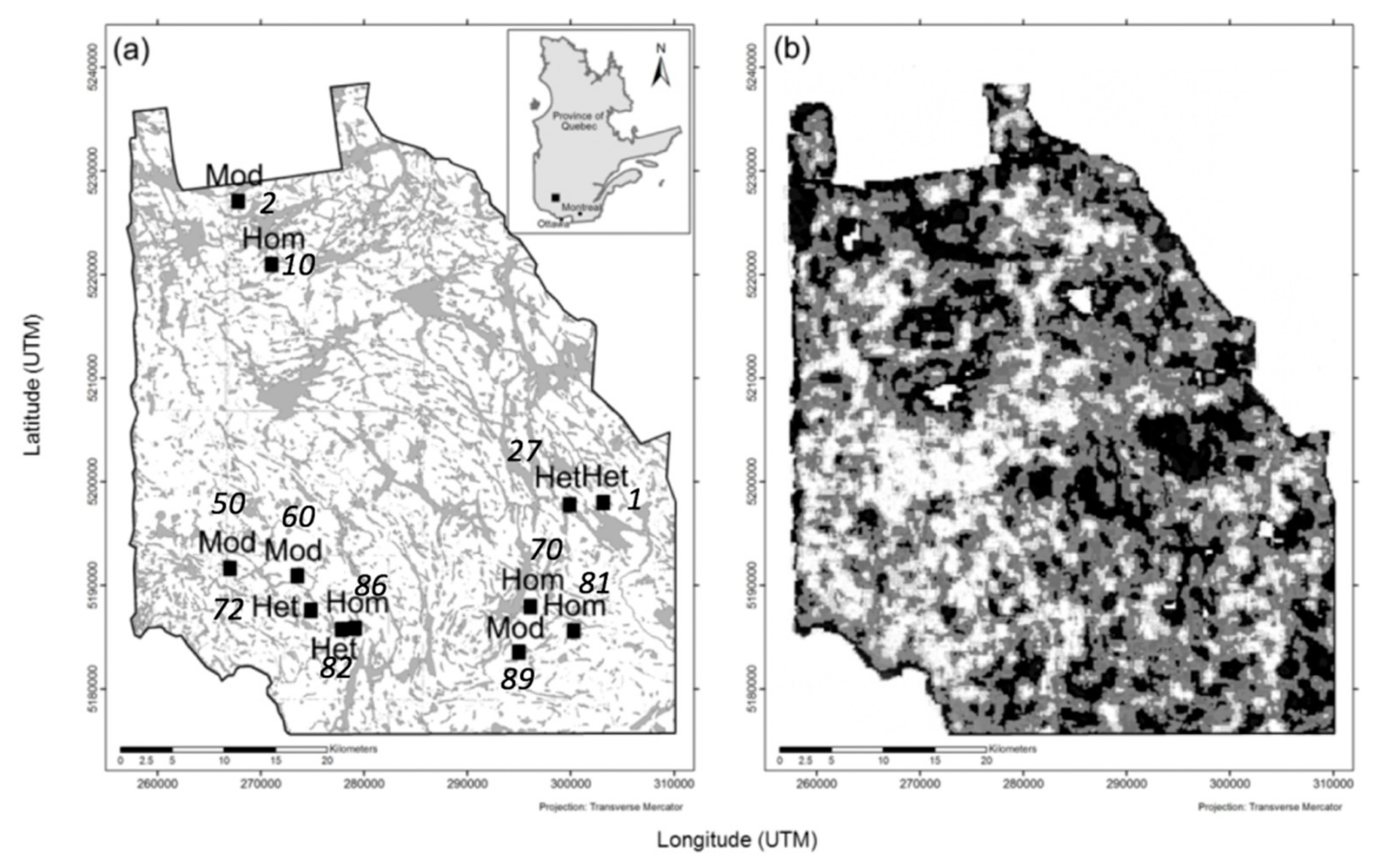
2.1. Study Area

Our study site was located in the La Verendrye wildlife reserve, which is part of the bF/yB bioclimatic domain [32]. The mixedwood forests in these areas are dominated by balsam fir (Abies balsamea (L.) Mill.), yellow birch (Betula alleghaniensis Britt.), white spruce (Picea glauca (Moench) Voss) and white birch (Betula papyrifera Marshall). Other species that occur in the study area include black spruce (Picea mariana (Mill.) Britton, Sterns & Poggenburg), white pine (Pinus strobus L.), eastern white cedar (Thuja occidentalis L.), trembling aspen (Populus tremuloides Michx.), red maple (Acer rubrum L. 1753) and sugar maple (Acer saccharum Marshall). The most abundant shrub species include mountain maple (Acer spicatum Lam. 1786), hazelnut (Corylus cornuta Marshall), hobblebush (Viburnum alnifolium Michx.) and wild raisin (Viburnum cassinoides L.).
In the La Verendrye wildlife reserve, the average elevation is 389 m, and the most common surface deposit is a thin layer of till overlying bedrock made of metamorphic rocks [32]. The mean annual precipitation in Maniwaki (40 km south of the sampled landscapes) is 908.8 mm (including 238.3 mm as snow) and the mean annual temperature is 3.7 °C. The southern mixedwood forests exhibit predominantly small-scale disturbances such as individual tree mortality, insect outbreaks and windthrow [33]. The natural fire cycle in western Québec is approximately 188 to 314 years, with historically longer fire cycles in the south and the east [34]. Large major spruce budworm outbreaks occurred in the region in 1910, 1945 and 1980 [35]. Fire suppression and a wetter climate in Québec since the 1920s has reduced the catastrophic disturbances that could reset the forest heterogeneity [34,36] while the use of clearcutting, which could play a similar role as fire, is quite limited in this area [37].
The dominant forest types of the bF/yB forests were managed using diameter-limited cuts from 1940 to 1980. Subsequently, selection cutting (single-tree and group) was proposed for managing them as uneven-aged stands [38,39]. In recent years, irregular shelterwood has been the prominent silvicultural system used for regenerating bF/yB forests [40]. Consequently, many stands of the bF/yB forests are now invaded by shrubs like mountain maple, hobblebush and hazelnut, and have become in some places a semi-permanent savannah-like ecosystem [41], now considered “degraded” forests [42].

2.2. Landscape Selection and Characterisation of Heterogeneity

We used ecoforest inventory maps from the province of Québec to assess landscape spatial heterogeneity. Ecoforest inventory maps contain polygons (> 4 ha) describing forest stands. We assigned a stand type to each stand by combining classes of forest overstory composition type (hardwood, mixedwood and softwood), stand cover density (25%–40%, 41%–60%, 61–80%, 81%–100%) and height (seven classes based on the height of dominant and codominant trees of the stand (1: >22m; 2: 17m–22m; 3: 12m–17m; 4: 7m–12m; 5: 4m–7m; 6: 2m–4m; 7: <2m). Adjacent polygons of the same stand type were merged. A stand type map was then created at a resolution of 1 ha and used to compute four subindices to represent different dimensions and scales of spatial heterogeneity. First, the mean size of the stand types was computed to account for landscape fragmentation; landscapes with smaller stand-type polygons were considered more heterogeneous [43]. The area-weighted cover density constituted the second subindex and allowed landscapes with more open stands to be distinguished, which provide more within-stand spatial heterogeneity than closed ones [44]. The third and fourth subindices represented stand type richness and stand type Shannon diversity index [45]. Each subindex was computed within a 100 ha circular sliding window, assigning the values to the focal cell, and was applied to the entire study region. Subindex values were standardized (0-1) and combined together, each subindex accounting for 25% of the landscape heterogeneity index (Table 1). The landscape heterogeneity index was then used to stratify the study area into three evenly represented classes of landscape heterogeneity: homogenous (0.18–0.37), moderate (0.38–0.61) and heterogeneous (0.62–0.77) (Figure 1b).
We then randomly selected a total of 12 landscapes (1 km2) for field sampling, 4 landscapes within each of the 3 landscape heterogeneity levels (homogenous, moderate and heterogeneous) (Figure 1a). Selected landscapes, although they had been subject to partial timber harvest in past decades, were dominated by mature forests; landscapes that had been too heavily or recently logged were avoided. Selected landscapes had to have a composition of at least 50% of yellow birch–balsam fir–white birch forest type. We selected landscapes with predominantly medium drainage regimes, from mainly (>75%) glacial till surficial deposits and < 10% standing water. All spatial analyses were completed using ArcGIS (ESRI 9.2, Redlands, CA, USA, 2006).

2.3. Field Sampling

Field sampling was conducted during the summer of 2010. Within each landscape, we randomly sampled 18 sites distributed along four 1 km transects in each landscape. Nine sites were under the forest canopy (radius = 11.28 m, area = 400 m²) and the other nine sites were in gaps of three different sizes (small (40–200 m²), medium (201–600 m²) and large (601 m² +)), each replicated three times. These four canopy closure environments are hereinafter referred to as the gap/forest environment factor for the statistical analysis. Canopy gap size was field measured assuming an elliptical shape (area = лab). Measurements of the axes were conducted assuming that the gap area ended at the vertical projection of the trees at the canopy edge. Trees had to be at least 75% the height of all the surrounding border gap trees to be considered part of the canopy border and not inside the gap.
Abundance and diversity measures were taken within four microquadrats of 5 m² (radius of 1.26 m) in the forest understory sites and four to eight microquadrats in the gaps, according to gap size (small = 4, medium = 6 and large = 8). Microquadrats were distributed along the northeast and northwest axes, taking into account the variability in light conditions due to the sunlight course in the gap. We recorded shrub total abundance (seedling: height ≥ 20 cm, diameter at 10 cm height < 1 cm, and sapling: diameter at 10 cm height ≥ 1.1 cm and ≤ 9 cm) and tree seedling (height ≥ 20 cm, diameter at 10 cm height < 1 cm) abundance by species in each microquadrat. Basal sprouts and stem layering when detected were counted as one individual.

2.4. Gap Proportion Assessment

Gap proportion in each forest landscape was assessed using LiDAR data according to the procedure described in Senécal et al. [46]. LiDAR was flown in 2015, using an Optech ALTM Gemini instrument operating at an average altitude of 650 m [47]. An average of 2.5 hits per m2 were recorded with a maximum half-scan angle of 18°, at a frequency of 55 Hz. Preprocessing of the LiDAR data included data cleaning, bird hit removal and classification of LiDAR points as ground surface hits. Canopy height models were generated at a resolution of 1 m (Figure 2). Bodies of water and recent harvest blocks (after 2010) were removed from the analyses. Identified gaps were classified in the same gap size classes that we used for the field sampling (40–200 m2, 201–600 m2 and 601 m2 +).

2.5. Statistical Analyses

2.5.1. Landscape Heterogeneity Characterization

Landscape heterogeneity subindices, as well as the global spatial landscape heterogeneity index made up of the combination of the four subindices, were tested against landscape heterogeneity level (homogeneous, moderate, heterogeneous) to examine how each subcomponent differed among the three classes we generated using the global spatial landscape heterogeneity index. Gap proportion in the different gap size classes was also tested against landscape heterogeneity level. These tests were conducted using one factor ANOVA (nlme and multcomp packages).

2.5.2. Alpha- and Beta-Diversity Characterization

We characterized alpha-diversity of shrubs and trees using the Shannon diversity index, calculated at the microquadrat level. Because diversity indices are sensitive to sampling area and given that our experimental design used unequal numbers of microquadrats per sampled gap size category (Supplementary Figure S1), we analyzed data at the 5-m2 microquadrat level. Alpha-diversity index data were analyzed using two factor ANOVA mixed models with landscape heterogeneity (heterogeneous, moderate and homogenous landscapes) and gap/forest environment (forest understory, small, medium and large gaps) as factors and the site identifier (sampled site (1–223)) as a random factor (using vegan, nlme and multcomp packages). Tukey tests were used to evaluate whether categories relevant to our hypotheses were different.
Beta-diversity was compared among heterogeneity levels by testing homogeneity of multivariate dispersions [48] using spatial median (vegan and betadisper packages). The analysis was performed for each gap/forest environment and for the two species groups (shrub and tree seedling) separately. Distance matrices were computed using Gower index (vegan and vegdist packages), which excluded double-zeros (meaning that two microquadrats both missing one species would not be considered more similar), on standardized (0–1) frequency (vegan and decostand packages). When homogeneity of multivariate dispersions was infirmed, Tukey’s “Honest Significant Difference” method was used to identify differences in beta-diversity between pair-wise comparisons of the three landscape heterogeneity levels.
We further characterized beta-diversity, using species accumulation curves of species for shrub and tree regeneration (vegan and specaccum packages). Species accumulation curves showing steeper slopes indicate greater beta-diversity [49]. As the relationship between abundance and local diversity led us to suspect a bias in species accumulation, rarefaction curves were thus generated to extract the species richness signal from the diversity-abundance effect (vegan and rarecurve packages). As rarefaction analysis is based on the number of individuals sampled rather than sampled area (m2), it is therefore not affected by uneven sample size [50]. Species-area and rarefaction curves were also computed by gap/forest environment. However, for testing the effect of landscape heterogeneity level, as the proportions of samples by gap/forest environment differ from those observed in the landscapes (Table 2), species accumulation and rarefaction curves of different landscape heterogeneity levels were drawn for each gap/forest environment separately. Significant difference was detected using a 95% confidence interval envelope and by making visual inferences [51,52]. All analyses were completed using R software (version 3.5.0 – “Joy in Playing”) (R Development Core Team: Vienna, Austria, 2019).

3. Results

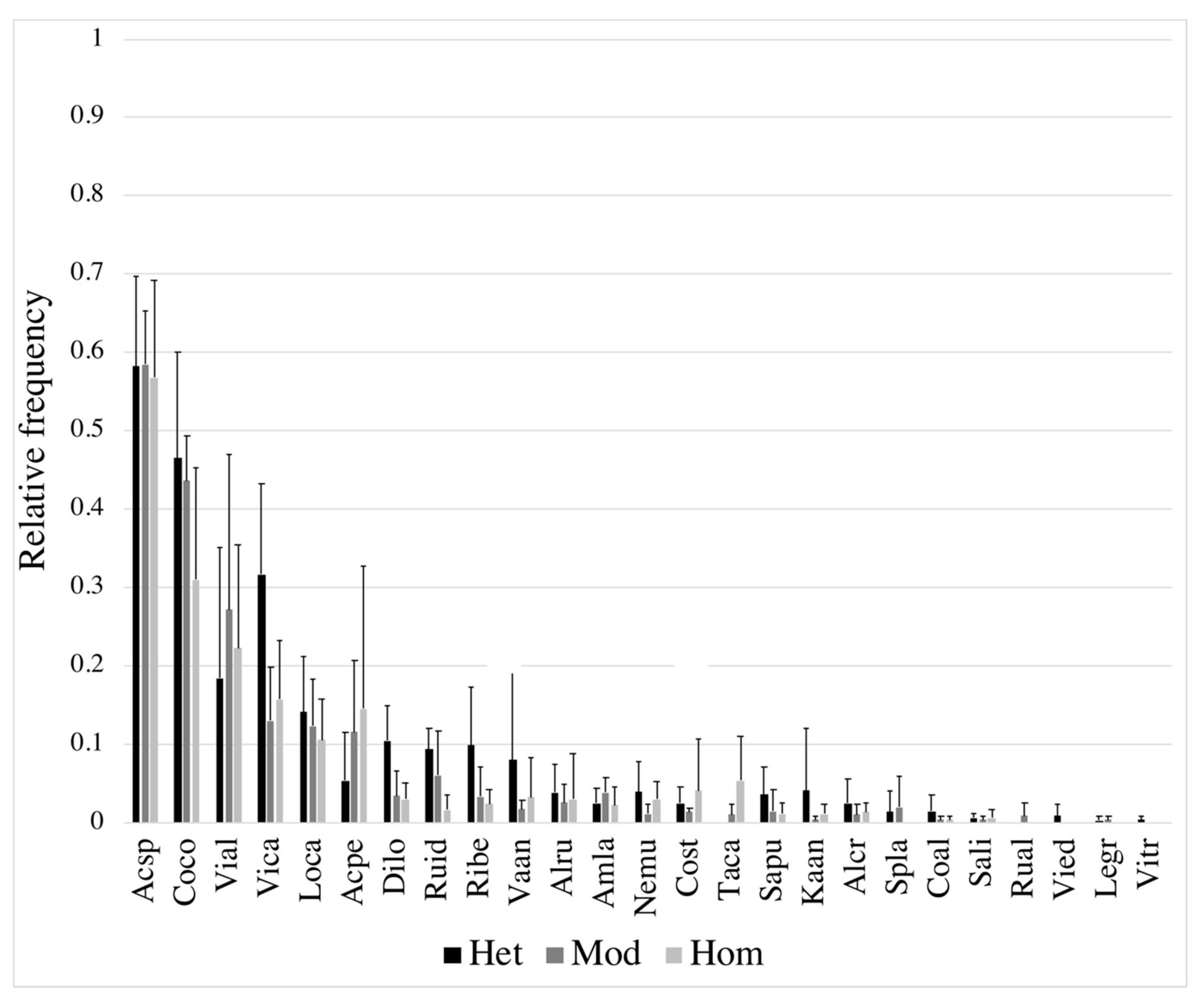
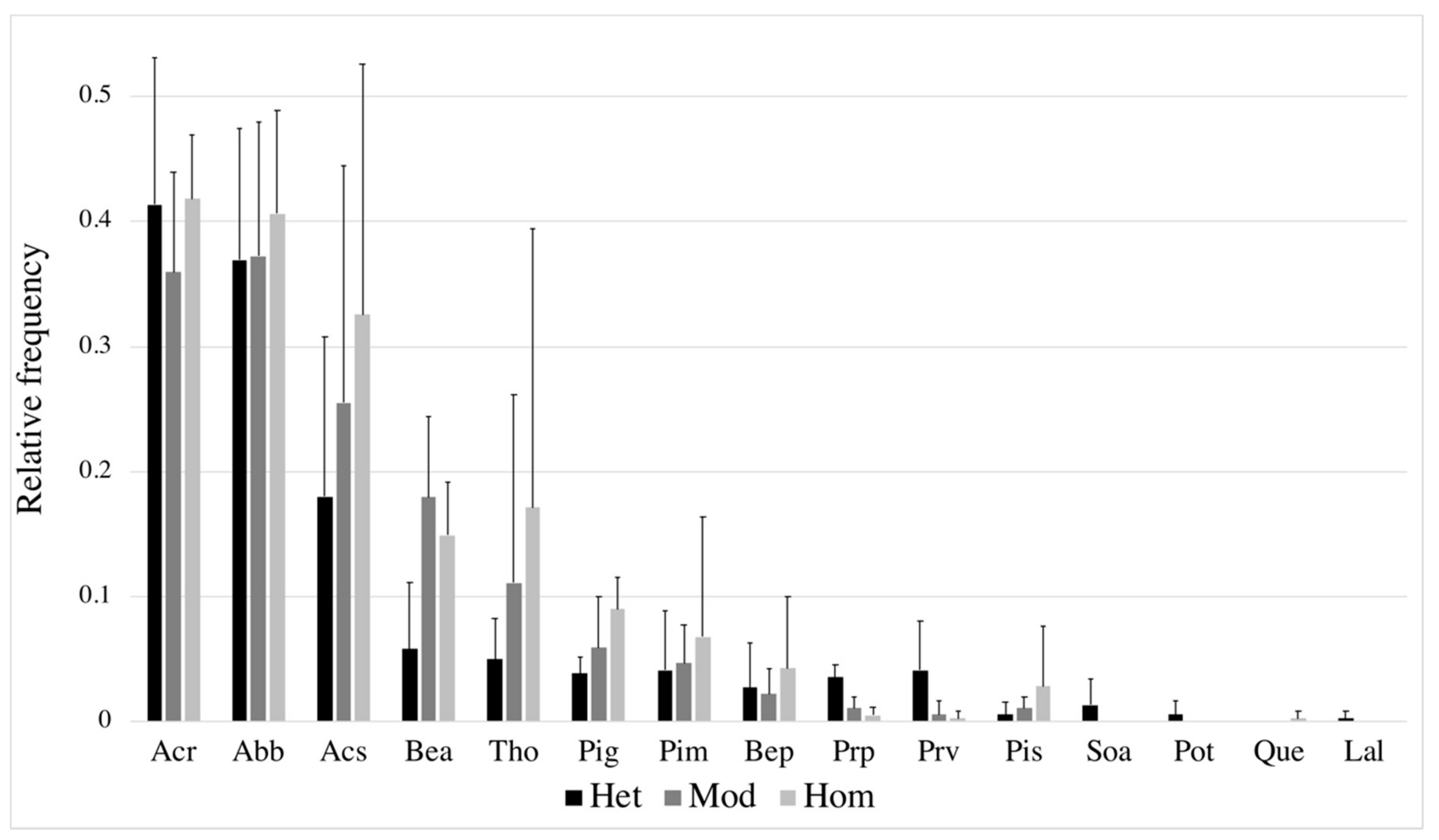
3.1. Effect of Landscape Heterogeneity

Most landscape heterogeneity subindices differed significantly among landscape heterogeneity levels (Table 1). The three levels of landscape heterogeneity were all significantly different from each other regarding their landscape spatial heterogeneity index values, with a difference of 0.2 between successive increasing classes of landscape heterogeneity level (Hom: 0.30, Mod: 0.50, Het: 0.69).
Small gaps (<200 m2) comprised around 80% of the openings in the landscapes we studied (Table 2). Gap proportion was significantly different among the landscape heterogeneity levels only for the largest gap size class (600–800 m2), which covered at least twice as much area in the heterogeneous landscapes as the two other landscape heterogeneity classes (Table 2). Nonetheless, the total proportion of gaps in the forests was not significantly different among landscape heterogeneity levels and sampled landscapes had on average 2.5% of their forested area in gaps.
The Shannon diversity index differed by gap/forest environment and landscape heterogeneity for shrubs and by landscape heterogeneity only for tree seedlings, with no significant interaction for both (Table 3). Shannon index shrub species were significantly more diverse in heterogeneous landscapes (2.38 species/microquadrat), when compared to either moderate (1.98 species/microquadrat), or homogenous landscapes (1.81 species/microquadrat) (Table 4). In contrast, the Shannon index for tree seedlings was significantly greater in homogenous landscapes (1.69 species/microquadrat) when compared to heterogeneous landscapes (1.28 species/microquadrat), but not against moderate heterogeneity landscapes (1.44 species/microquadrat).
We found a negative relationship between shrub abundance and tree seedling diversity using simple regression (T value = −3.71, P(f) = <0.01). Acer spicatum was the most frequent shrub species and was equally frequent (around 55%) in all landscape heterogeneity levels (Figure 3). Other shrub species were usually more frequent in the heterogeneous landscapes, with the exception of Viburnum alnifolium, Acer pensylvanicum L. 1753 and Taxus Canadensis Marshall, three shade-tolerant shrubs. Acer rubrum and Abies balsamea were the most frequent tree seedling species in all landscape types (Figure 4). The shade-tolerant tree seedling species Acer saccharum, and Thuja occidentalis, and the mid-tolerant softwood species Picea glauca and Pinus strobus were less frequent in heterogeneous landscapes, while early pioneer species like Prunus pensylvanica, Prunus virginiana, Sorbus americana and Populus tremuloides were more frequent in heterogeneous landscapes. Moderately heterogeneous landscapes were characterized by a higher frequency of the mid-shade-tolerant Betula alleghaniensis.
Beta-diversity, as measured by multivariate dispersion, was significantly different among landscape heterogeneity levels in the forest understory environment for the shrub species group (F value = 6.11, P(f) < 0.01), but not for any other gap/forest environment, and was higher in heterogeneous landscapes than in homogeneous landscapes (Table 5, Supplementary Figure S1). Species accumulation rate was greatest in heterogeneous landscapes in the forest understory, and small-, and medium-size gap environments (Figure 5a–c). However, because of the important width of the envelope of confidence intervals, a significantly higher species accumulation rate was only detectable within medium gaps in heterogeneous landscapes (Figure 5c). For medium sized-gaps, the difference in species–area curves was significant (alpha = 0.05%) between heterogeneous and homogenous landscapes (Figure 5c). Rarefaction curves supported these results and produced a similar pattern showing heterogeneous landscapes to have the highest species accumulation rates for shrubs in the forest understory, and small- and medium-sized gaps (Supplementary Figure S2a–c), but not for large gaps (Supplementary Figure S2d).
Tree seedling beta-diversity, as measured by multivariate dispersion, did not differ among landscape heterogeneity levels for any of the landscape heterogeneity gap/forest environment interactions (Table 5, Supplementary Figure S1). For tree regeneration, the species area accumulation curve appeared to be higher for heterogeneous landscapes when compared to moderate ones in forest understories (Figure 5e). Rarefaction curves for tree seedlings appeared to confirm that species accumulation was highest in heterogeneous landscapes within the forest understory (Supplementary Figure S2e).

3.2. Diversity in Response to Gap/Forest Environment

The Shannon diversity index for shrub species was greatest in gaps, whatever their size class, when compared to the forest understory (Table 4). However, tree seedling species diversity did not respond significantly to the gap–understory gradient (Table 3). In general, beta-diversity, as measured by multivariate dispersion, had higher values in gaps than in the forest understory, whatever the species group (Table 5). For shrub species, we observed a slightly lower but non-significant species accumulation, by area or by sample size, in forest understory than in small- and large-sized gaps (Figure 6a, Supplementary Figure S3a). For tree seedling species, a greater accumulation rate appeared in small gaps, but the difference with the three other gap/forest environments was not significant (Figure 6b, Supplementary Figure S3b).

4. Discussion

4.1. Heterogeneity–Diversity Relationship or Biotic Interaction?

As expected, a HDR was observed for shrubs. Shrub species alpha-diversity was greatest in heterogeneous landscapes when compared to the two other landscape heterogeneity levels, and species richness was greatest by 0.4 and 0.57 species/microquadrat (5m2) within these two landscape heterogeneity levels, respectively. Not only was alpha-diversity greater, but species turnover (beta-diversity) was generally higher in heterogeneous landscapes for the shrub species group, particularly in the forest understory environment. Environmental heterogeneity is thought to enhance biodiversity through greater niche space [3,20]. Indeed, landscape heterogeneity is thought to increase species diversity by augmenting the regional species pool of species available to colonize new resource-rich habitats [7,9]. For example, landscape heterogeneity associated with anthropogenic and/or natural disturbance has been shown to promote species richness in central Europe [53]. Landscape heterogeneity as measured by edge density and patch size was found to promote species richness in the boreal mixedwoods of eastern Canada [10]. Landscape heterogeneity has also been found to increase species richness in montane wooded pastures and semi-natural grasslands of Europe [8,9,11,54,55]. Similarly, agricultural weed species diversity has been shown to increase as the number of fields increased and field size decreased, and as habitat-type diversity, topographical heterogeneity and the perimeter–area ratio increases [14,15]. However, the mechanisms influencing diversity between natural grasslands and forests differ; grassland patterns are caused by the homogenization and intensification of agriculture, whereas in the southern mixedwood forests, recurrent anthropogenic and natural disturbances increase landscape heterogeneity [43,56].
In contrast to shrubs, we found lower tree regeneration alpha-diversity in heterogeneous landscapes when compared to homogeneous landscapes. We believe that this reduction in tree alpha-diversity is due to high shrub abundance in heterogeneous landscapes [57]. For beta-diversity, no specific pattern of multivariate dispersion was detectable for tree seedlings, but species accumulation curves (by sample area or by number of individuals) showed greater turnover rates in heterogeneous landscapes in the forest understory. As the forest understory is the most common environment (a total 97.5% of the area for all landscapes we studied), we argue that beta-diversity was greatest in heterogeneous landscapes overall, giving partial support to the HDR hypothesis for this species group. These results show negative alpha-diversity and positive beta-diversity response of tree seedlings toward landscape heterogeneity; a predominantly positive beta-diversity response of tree seedlings to landscape heterogeneity suggests positive niche effects overriding local competitive effects. Tree beta-diversity increases with light heterogeneity in Mexican tropical forests [30]. Landscape complexity (measured as the perimeter/area ratio of cropland) positively influences plant beta-diversity in farmland due to spatial heterogeneity of fencerows maintaining diversity in agro-ecosystems [12]. Abiotic variation can be expected to influence species diversity at broad scales, while habitat types could be more influential at finer landscape scales [54].
A negative HDR has been identified by other authors [58,59,60,61]. These authors have explained negative HDRs by the presence of plants exhibiting a competitive advantage in heterogeneous environments, causing some species to dominate and thus reducing species diversity. This mechanism is referred to as a separate heterogeneity niche axis, and we believe shrubs in our study were able to exploit this niche [59]. For example, when resource patches are smaller than a species’ minimal space requirement, species need to be able to exploit different resource patches at the same time in order to be unaffected by heterogeneity [58,59]. Alternatively, the area–heterogeneity tradeoff postulates that heterogeneity will promote favorable conditions for a large number of species with differing niche requirements; however, smaller patch sizes decrease population size and increase the likelihood of random extinction [62,63]. Given these mechanisms for negative HDR, it is also possible that a quadratic relationship best describes this association, providing peak diversity at intermediate levels of heterogeneity [63,64]. Forests dominated by species with narrow niche width (specialists) would respond negatively to heterogeneity, while species with wide niches (generalists) would show mostly positive response [63].

4.2. Diversity–Resource Relationship and Species Traits

We hypothesized that species richness for both shrub and tree seedling species groups should increase with gap area, because larger gaps have higher resource levels and more microsite heterogeneity than small gaps [28,29]. Shrubs were more diverse in our study in resource-rich gaps when compared to the forest understory; this was consistent with shrubs possessing traits more adapted to disturbances, including persistence followed by fast vegetative growth for rapid colonization of newly created habitat patches [16,17]. Our results were thus consistent with the expectation of greater shrub diversity in shifting landscape mosaic with high spatiotemporal environmental heterogeneity [3,18,19,20]. In contrast to shrubs, tree seedlings, although they were more abundant in the forest understory and in small gaps [57], were not more diverse in any of the gap/forest environments, consistent with longevity dominance traits that permit them to dominate both regionally and locally (97.5% of the area is closed-canopy-tree dominated) [22]. Our results were also consistent with those of References [24,57], who suggested that lower tree seedling density in heterogeneous landscapes is due to competition with shrubs. However, when understory species are suppressed by overstory trees, this in turn reduces negative effects on understory richness [65,66].

5. Conclusions

Our work provides evidence that landscape spatial heterogeneity influences woody species diversity in the balsam fir/yellow birch bioclimatic domain. At the local scale, we found that alpha-diversity was greater for shrubs but lower for tree regeneration in heterogeneous landscapes. Despite such an effect at the local scale, greater beta-diversity in heterogeneous landscapes was detected for both species groups.
We suspect that the recalcitrant layer invasion of the competitive shrub species group may be ongoing and progressing. If so, competitive vegetative fast-growing shrub populations could keep on building up, reducing not only tree seedling diversity locally but also species turnover rate in heterogeneous landscapes. Cumulated disturbances from forest management and natural disturbances are likely to continue increasing the pace of the shifting mosaic dynamic in these landscapes in the near future, as the spruce budworm is now reaching an epidemic phase [67]. These results are important because forest managers must not assume that heterogeneous environments will always benefit diversity; negative diversity–heterogeneity effects have been observed and, in our case, local competitive interactions can complicate matters. We believe that the studied area surpassed a threshold level of heterogeneity that is beneficial for diversity, and despite the dominance of tree cover could be progressing towards an extreme that allows for a recalcitrant understory layer to reduce tree diversity in heterogeneous landscapes.

Supplementary Materials

The following are available online at https://www.mdpi.com/1999-4907/11/2/160/s1, Table S1. Sum of microquadrats (a) and sites (b) considering the two main effects of landscape heterogeneity, gap/forest environment and their interaction. Figure S1. Box-plot of the multivariate distance to the spatial mean (centroid) for shrub (a to d) and tree seedling (e to h) species groups in landscapes of different heterogeneity levels (heterogeneous (Het), moderate (Mod), homogenous (Hom)) for different gap/forest environments (forest (F) understory, small (S) gaps, medium (M) gaps, large (L) gaps). Figure S2. Species rarefaction curves from landscapes with different spatial heterogeneity levels (heterogeneous (Het), moderate (Mod), homogenous (Hom)) in four distinct gap/forest environments (forest (F) understory, small (S) gaps, medium (M) gaps, large (L) gaps) for shrub (a to d) and tree seedling (e to h) species. Figure S3. Species rarefaction curves from four distinct gap/forest environments (forest (F) understory, small (S) gaps, medium (M) gaps, large (L) gaps) for shrub (a) and tree seedling (b) species.

Author Contributions

Conceptualization, R.M., F.D. and D.K.; Data curation, R.M. and F.D.; Formal analysis, R.M. and F.D.; Funding acquisition, R.M., F.D. and D.K.; Writing—original draft, R.M., F.D. and D.K.; Writing—review & editing, R.M., F.D. and D.K. All authors have read and agreed to the published version of the manuscript.

Funding

This project was funded by the Ministère des forêts, de la faune et des parcs (MFFP), Fonds de recherche du Québec nature et technologies (FRQNT), MiTACS and Nova Sylva inc.

Acknowledgments

We would like to thank Jean-François Senécal for his help in providing the data for calculating gap proportion by size class from the canopy height model derived from aerial LiDAR data and for producing Figure 2. We would also like to thank Marie-Ève Roy, Régis Pouliot, Pascal Rochon, Nadia Bergeron and Louis Gauthier for statistical help and fieldwork. A special thank you to Marc Mazerolle for help with statistics.

Conflicts of Interest

The authors declare no conflict of interest. The funders had no role in the design of the study; in the collection, analyses, or interpretation of data; in the writing of the manuscript, or in the decision to publish the results.

References

  1. Levin, S.A. The problem of pattern and scale in ecology: The Robert H. MacArthur award lecture. Ecology 1992, 73, 1943–1967. [Google Scholar] [CrossRef]
  2. Whittaker, R.J.; Willis, K.J.; Field, R. Scale and species richness: towards a general, hierarchical theory of species diversity. J. Biogeogr. 2001, 28, 453–470. [Google Scholar] [CrossRef] [Green Version]
  3. Sarr, D.A.; Hibbs, D.E.; Huston, M.A. A hierarchical perspective of plant diversity. Q. Rev. Biol. 2005, 80, 187–212. [Google Scholar] [CrossRef] [PubMed]
  4. Turner, M.G. Landscape ecology: the effect of pattern on process. Annu. Rev. Ecol. S. 1989, 20, 171–197. [Google Scholar] [CrossRef]
  5. Wiens, J.A. Ecological heterogeneity: an ontogeny of concepts and approaches. In The Ecological Consequences of Environmental Heterogeneity; Hutchings, M.J., John, E.A., Stewart, A.J.A., Eds.; Blackwell Science: Oxford, UK, 2000; pp. 9–31. [Google Scholar]
  6. Fahrig, L.; Baudry, J.; Brotons, L.; Burel, F.G.; Crist, T.O.; Fuller, R.J.; Sirami, C.; Siriwardena, G.M.; Martin, J.L. Functional landscape heterogeneity and animal biodiversity in agricultural landscapes. Ecol. Lett. 2010, 14, 101–112. [Google Scholar] [CrossRef]
  7. Tscharntke, T.; Tylianakis, J.M.; Rand, T.A.; Didham, R.K.; Fahrig, L.; Batary, P.; Bengtsson, J.; Clough, Y.; Crist, T.O.; Dormann, C.F.; et al. Landscape moderation of biodiversity patterns and processes-eight hypotheses. Biol. Rev. 2012, 87, 661–685. [Google Scholar] [CrossRef]
  8. Gámez-Virués, S.; Perović, D.J.; Gossner, M.M.; Börschig, C.; Blüthgen, N.; De Jong, H.; Simons, N.K.; Klein, A.M.; Krauss, J.; Maier, G.; et al. Landscape simplification filters species traits and drives biotic homogenization. Nat. Commun. 2015, 6, 8568. [Google Scholar]
  9. Sutcliffe, L.M.; Batáry, P.; Becker, T.; Orci, K.M.; Leuschner, C. Both local and landscape factors determine plant and Orthoptera diversity in the semi-natural grasslands of Transylvania, Romania. Biodivers. Conserv. 2015, 24, 229–245. [Google Scholar] [CrossRef]
  10. Kumar, S.; Stohlgren, T.J.; Chong, G.W. Spatial heterogeneity influences native and nonnative plant species richness. Ecology 2006, 87, 3186–3199. [Google Scholar] [CrossRef]
  11. Dufour, A.; Gadallah, F.; Wagner, H.H.; Guisan, A.; Buttler, A. Plant species richness and environmental heterogeneity in a mountain landscape: effects of variability and spatial configuration. Ecography 2006, 29, 573–584. [Google Scholar] [CrossRef]
  12. Poggio, S.L.; Chaneton, E.J.; Ghersa, C.M. Landscape complexity differentially affects alpha, beta, and gamma diversities of plants occurring in fencerows and crop fields. Biol. Conserv. 2010, 143, 2477–2486. [Google Scholar] [CrossRef]
  13. Zelený, D.; Li, C.F.; Chytrý, M. Pattern of local plant species richness along a gradient of landscape topographical heterogeneity: result of spatial mass effect or environmental shift? Ecography 2010, 33, 578–589. [Google Scholar] [CrossRef]
  14. Gabriel, D.; Thies, C.; Tscharntke, T. Local diversity of arable weeds increases with landscape complexity. Perspect. Plant Ecol. 2005, 7, 85–93. [Google Scholar] [CrossRef]
  15. Gaba, S.; Chauvel, B.; Dessaint, F.; Bretagnolle, V.; Petit, S. Weed species richness in winter wheat increases with landscape heterogeneity. Agr. Ecosyst. Environ. 2010, 138, 318–323. [Google Scholar] [CrossRef]
  16. Young, T.P.; Peffer, E. “Recalcitrant understory layers” revisited: arrested succession and the long life-spans of clonal mid-successional species. Can. J. For. Res. 2010, 40, 1184–1188. [Google Scholar] [CrossRef]
  17. Valladares, F.; Guzmán, B. Canopy structure and spatial heterogeneity of understory light in an abandoned Holm oak woodland. Ann. For. Sci. 2006, 63, 749–761. [Google Scholar] [CrossRef] [Green Version]
  18. Leibold, M.A.; McPeek, M.A. Coexistence of the niche and neutral perspectives in community ecology. Ecology 2006, 87, 1399–1410. [Google Scholar] [CrossRef]
  19. Adler, P.B.; HilleRisLambers, J.; Levine, J.M. A niche for neutrality. Ecol. Lett. 2007, 10, 95–104. [Google Scholar] [CrossRef] [Green Version]
  20. Stein, A.; Gerstner, K.; Kreft, H. Environmental heterogeneity as a universal driver of species richness across taxa, biomes and spatial scales. Ecol. Lett. 2014, 17, 866–880. [Google Scholar] [CrossRef]
  21. Grace, J.B. The factors controlling species density in herbaceous plant communities: an assessment. Perspect. Plant Ecol. 1999, 2, 1–28. [Google Scholar] [CrossRef]
  22. Woods, K.D. Intermediate disturbance in a late-successional hemlock-northern hardwood forest. J. Ecol. 2004, 92, 464–476. [Google Scholar] [CrossRef]
  23. Kneeshaw, D.D.; Prévost, M. Natural canopy gap disturbances and their role in maintaining mixed-species forests of central Québec, Canada. Can. J. For. Res. 2007, 37, 1534–1544. [Google Scholar] [CrossRef]
  24. Royo, A.A.; Carson, W.P. On the formation of dense understory layers in forests worldwide: consequences and implications for forest dynamics, biodiversity, and succession. Can. J. For. Res. 2006, 36, 1345–1362. [Google Scholar] [CrossRef]
  25. De Blois, S.; Domon, G.; Bouchard, A. Landscape issues in plant ecology. Ecography 2002, 25, 244–256. [Google Scholar] [CrossRef]
  26. Kern, C.C.; Montgomery, R.A.; Reich, P.B.; Strong, T.F. Harvest-created canopy gaps increase species and functional trait diversity of the forest ground-layer community. Forest Science 2014, 60, 335–344. [Google Scholar] [CrossRef]
  27. Busing, R.T.; Brokaw, N. Tree species diversity in temperate and tropical forest gaps: the role of lottery recruitment. Folia Geobot. 2002, 37, 33–43. [Google Scholar] [CrossRef]
  28. Muscolo, A.; Bagnato, S.; Sidari, M.; Mercurio, R. A review of the roles of forest canopy gaps. J. For. Res. 2014, 25, 725–736. [Google Scholar] [CrossRef]
  29. Raymond, P.; Royo, A.A.; Prévost, M.; Dumais, D. Assessing the single-tree and small group selection cutting system as intermediate disturbance to promote regeneration and diversity in temperate mixedwood stands. Forest Ecol. Manag. 2018, 430, 21–32. [Google Scholar] [CrossRef]
  30. Balvanera, P.; Lott, E.; Segura, G.; Siebe, C.; Islas, A. Patterns of beta-diversity in a Mexican tropical dry forest. J. Veg. Sci. 2002, 13, 145–158. [Google Scholar] [CrossRef]
  31. Alahuhta, J.; Kosten, S.; Akasaka, M.; Auderset, D.; Azzella, M.M.; Bolpagni, R.; Bove, C.P.; Chambers, P.A.; Chappuis, E.; Clayton, J.; et al. Global variation in the beta diversity of lake macrophytes is driven by environmental heterogeneity rather than latitude. J. Biogeogr. 2017, 44, 1758–1769. [Google Scholar] [CrossRef]
  32. Robitaille, A.; Saucier, J.-P. Paysages régionaux du Québec méridional; Les Publications du Québec: Québec, QC, Canada, 1998. [Google Scholar]
  33. Prévost, M.; Roy, V.; Raymond, P. Sylviculture et régénération des forêts mixtes du Québec (Canada): une approche qui respecte la dynamique naturelle des peuplements; Direction de la recherche forestière, Ministère des ressources naturelles: Québec, QC, Canada, 2003. [Google Scholar]
  34. Grenier, D.; Bergeron, Y.; Kneeshaw, D.; Gauthier, S. Fire frequency for the transitional mixedwood forest of Timiskaming, Québec, Canada. Can. J. For. Res. 2005, 35, 656–666. [Google Scholar] [CrossRef]
  35. Bouchard, M.; Kneeshaw, D.; Bergeron, Y. Forest dynamics after successive spruce budworm outbreaks in mixedwood forests. Ecology 2006, 87, 2319–2329. [Google Scholar] [CrossRef]
  36. Cumming, S.G. Effective fire suppression in boreal forests. Can. J. For. Res. 2005, 35, 772–786. [Google Scholar] [CrossRef]
  37. Boucher, Y. Registre des états de référence; Direction de la recherche forestiére, Gouvernement du Québec: Québec, QC, Canada, 2011. [Google Scholar]
  38. Robitaille, L.; Majcen, Z. Traitements sylvicoles visant à favoriser la régénération et la croissance du bouleau jaune. L’Aubelle 1991, 82, 10–12. [Google Scholar]
  39. Majcen, Z. Historique des coupes de jardinage dans les forêts inéquiennes au Québec. Rev. For. Fr. 1994, 4, 375–384. [Google Scholar] [CrossRef] [Green Version]
  40. Raymond, P.; Dumais, D.; Prévost, M. Écologie et sylviculture la forêt mixte: Qu’avons-nous appris au cours de la dernière décennie? Carrefour Forêt Innovations: Québec, QC, Canada, 2012. [Google Scholar]
  41. Gastaldello, P.; Ruel, J.C.; Lussier, J.M. Remise en production des bétulaies jaunes résineuses dégradées: étude du succès d’installation de la régénération. For. Chron. 2007, 83, 742–753. [Google Scholar] [CrossRef] [Green Version]
  42. Roy, V.; Prévost, M. Caractérisation des bétulaies jaunes résineuses dégradées de la sapinière à bouleau jaune; Programme de mise en valeur des ressources du milieu forestier, Volet 1: Québec, QC, Canada, 2001. [Google Scholar]
  43. Bresee, M.K.; Le Moine, J.; Mather, S.; Brosofske, K.D.; Chen, J.; Crow, T.R.; Rademacher, J. Disturbance and landscape dynamics in the Chequamegon National Forest Wisconsin, USA, from 1972 to 2001. Landsc. Ecol. 2004, 19, 291–309. [Google Scholar] [CrossRef]
  44. Peck, J.E.; Zenner, E.K.; Brang, P.; Zingg, A. Tree size distribution and abundance explain structural complexity differentially within stands of even-aged and uneven-aged structure types. Eur. J. Forest Res. 2014, 133, 335–346. [Google Scholar] [CrossRef]
  45. McElhinny, C.; Gibbons, P.; Brack, C.; Bauhus, J. Forest and woodland stand structural complexity: its definition and measurement. Forest Ecol. Manag. 2005, 218, 1–24. [Google Scholar] [CrossRef]
  46. Senécal, J.F.; Doyon, F.; Messier, C. Management implications of varying gap detection height thresholds and other canopy dynamics processes in temperate deciduous forests. Forest Ecol. Manag. 2018, 410, 84–94. [Google Scholar] [CrossRef]
  47. MFFP. Guide d’utilisation des produits dérivés du LiDAR; Direction des inventaires forestiers, Ministère des Forêts, de la Faune et des Parcs, Secteur des forêts: Québec, QC, Canada, 2016. [Google Scholar]
  48. Anderson, M.J. Distance-based tests for homogeneity of multivariate dispersions. Biometrics 2006, 62, 245–253. [Google Scholar] [CrossRef] [PubMed]
  49. Scheiner, S.M. A mélange of curves – further dialogue about species – area relationships. Glo. Ecol. Biogeogr. 2004, 13, 479–484. [Google Scholar] [CrossRef]
  50. Gotelli, N.J.; Colwell, R.K. Estimating species richness. Biological diversity: frontiers in measurement and assessment 2011, 12, 39–54. [Google Scholar]
  51. Cumming, G. Inference by eye: Pictures of confidence intervals and thinking about levels of confidence. Teaching Statistics 2007, 29, 89–93. [Google Scholar] [CrossRef]
  52. R Development Core Team. R: A language and environment for statistical computing; R Foundation for Statistical Computing: Vienna, Austria, 2014. [Google Scholar]
  53. Deutschewitz, K.; Lausch, A.; Kühn, I.; Klotz, S. Native and alien plant species richness in relation to spatial heterogeneity on a regional scale in Germany. Glob. Ecol. Biogeogr. 2003, 12, 299–311. [Google Scholar] [CrossRef] [Green Version]
  54. Hofer, G.; Wagner, H.H.; Herzog, F.; Edwards, P.J. Effects of topographic variability on the scaling of plant species richness in gradient dominated landscapes. Ecography 2008, 31, 131–139. [Google Scholar] [CrossRef] [Green Version]
  55. Loos, J.; Turtureanu, P.D.; von Wehrden, H.; Hanspach, J.; Dorresteijn, I.; Frink, J.P.; Fischer, J. Plant diversity in a changing agricultural landscape mosaic in Southern Transylvania (Romania). Agr. Ecosyst. Environ. 2015, 199, 350–357. [Google Scholar] [CrossRef]
  56. McGarigal, K.; Romme, W.H.; Crist, M.; Roworth, E. Cumulative effects of roads and logging on landscape structure in the San Juan Mountains, Colorado (USA). Landsc. Ecol. 2001, 16, 327–349. [Google Scholar] [CrossRef]
  57. Markgraf, R.; Doyon, F.; Roy, M.È.; Kneeshaw, D. Landscape heterogeneity influences tree and shrub species abundance while local gap environments influence growth in temperate mixedwood forests. Under review.
  58. Lundholm, J.T. Plant species diversity and environmental heterogeneity: spatial scale and competing hypotheses. J. Veg. Sci. 2009, 20, 377–391. [Google Scholar] [CrossRef]
  59. Tamme, R.; Hiiesalu, I.; Laanisto, L.; Szava-Kovats, R.; Pärtel, M. Environmental heterogeneity, species diversity and co-existence at different spatial scales. J. Veg. Sci. 2010, 21, 796–801. [Google Scholar] [CrossRef]
  60. Costanza, J.K.; Moody, A.; Peet, R.K. Multi-scale environmental heterogeneity as a predictor of plant species richness. Lands. Ecol. 2011, 26, 851–864. [Google Scholar] [CrossRef]
  61. Gazol, A.; Tamme, R.; Takkis, K.; Kasari, L.; Saar, L.; Helm, A.; Pärtel, M. Landscape- and small-scale determinants of grassland species diversity: direct and indirect influences. Ecography 2012, 35, 944–951. [Google Scholar] [CrossRef]
  62. Clavel, J.; Julliard, R.; Devictor, V. Worldwide decline of specialist species: toward a global functional homogenization? Front. Ecol. Environ. 2011, 9, 222–228. [Google Scholar] [CrossRef] [Green Version]
  63. Allouche, O.; Kalyuzhny, M.; Moreno-Rueda, G.; Pizarro, M.; Kadmon, R. Area–heterogeneity tradeoff and the diversity of ecological communities. Proc. Natl. Acad. Sci. 2012, 109, 17495–17500. [Google Scholar] [CrossRef] [PubMed] [Green Version]
  64. Redon, M.; Berges, L.; Cordonnier, T.; Luque, S. Effects of increasing landscape heterogeneity on local plant species richness: how much is enough? Landsc. Ecol. 2014, 29, 773–787. [Google Scholar] [CrossRef]
  65. Bartels, S.F.; Chen, H.Y. Is understory plant species diversity driven by resource quantity or resource heterogeneity? Ecology 2010, 91, 1931–1938. [Google Scholar] [CrossRef]
  66. Reich, P.B.; Frelich, L.E.; Voldseth, R.A.; Bakken, P.; Adair, E.C. Understorey diversity in southern boreal forests is regulated by productivity and its indirect impacts on resource availability and heterogeneity. J. Ecol. 2012, 100, 539–545. [Google Scholar] [CrossRef]
  67. Mingke, L.I.; Maclean, D.A.; Hennigar, C.R.; Ogilvie, J. Previous year outbreak conditions and spring climate predict spruce budworm population changes in the following year. Forest Ecol. Manag. 2019, 117737. [Google Scholar]
Figure 1. Geographical position of the 12 sample landscapes (a) (grey areas are waterbodies and waterways; italicised numbers represent landscape identifier) and map of the spatial landscape heterogeneity index (b) (heterogeneous: white; moderate: grey; homogenous: black).
Forests 11 00160 g001
Figure 2. Example (landscape no. 89, see Figure 1a for its exact position in the southeast of the study area) of a canopy height model derived from aerial LiDAR data used to detect forest gaps (hatched zones in the insert) (gap height threshold = 5 m).
Forests 11 00160 g002
Figure 3. Relative frequencies of the shrub species in the three different landscape heterogeneity levels (heterogeneous (Het, n = 4), moderate (Mod, n = 4) and homogenous (Hom, n = 4)). Error bars represent confidence intervals (alpha = 0.05%). Acsp: Acer spicatum; Coco: Corylus cornuta; Vial: Viburmum alnifolium; Vica: Viburnum cassinoides; Loca: Lonicera canadensis; Acpe: Acer pensylvanicum; Dilo: Diervilla lonicera; Ruid: Rubus ideaeus; Ribe: Ribes spp.; Vaan: Vaccinium angustifolium; Alru: Alnus rugosa; Amla: Amelanchier leavis; Nemu: Nemopanthus mucronata; Cost: Cornus stolonifera; Taca: Taxus canadensis; Sapu: Sambucus pubescens; Kaan: Kalmia angustifolia; Alcr: Alnus crispa; Spla: Spirea latifolia; Coal: Cornus alternifolia; Sali: Salix spp.; Rual: Rubus alleghaniensis; Vied: Viburnum edule; Legr: Ledum groenlandicum; Vitr: Viburnum trilobata.
Forests 11 00160 g003
Figure 4. Relative frequencies of the tree seedling species in the three different landscape heterogeneity levels (heterogeneous (Het, n = 4), moderate (Mod, n = 4), homogenous (Hom, n = 4)). Error bars represent confidence intervals (alpha = 0.05%). Acr: Acer rubrum; Abb: Abies balsamea; Acs: Acer saccharum; Bea: Betula alleghaniensis; Tho: Thuya occidentalis; Pig: Picea glauca; Pim: Picea mariana; Bep: Betula papyrifera; Prp: Prunus pensylvanica; Prv: Prunus virginiana; Pis: Pinus strobus; Soa: Sorbus americana; Pot: Populus tremuloides; Que Quercus rubra; Lal: Larix laricina.
Forests 11 00160 g004
Figure 5. Species accumulation curves from landscapes with different spatial heterogeneity levels (heterogeneous (Het), moderate (Mod), homogenous (Hom)) in four distinct gap/forest environments (forest (F) understory, small (S) gaps, medium (M) gaps, large (L) gaps) for shrub (a)–(d) and tree seedling (e)–(h) species. Envelopes show boot-strapped 95% confidence intervals.
Forests 11 00160 g005aForests 11 00160 g005b
Figure 6. Species accumulation curves from four gap/forest environments (forest (F) understory, small (S) gaps, medium (M) gaps, large (L) gaps) for shrub (a) and tree seedling (b) species. Envelopes show boot-strapped 95% confidence intervals.
Forests 11 00160 g006
Table 1. Landscape heterogeneity indices of the 12 sampled landscapes. Means with different letters (column-wise) are significantly different.
Landscape No.Heterogeneity LevelStand Type Shannon Diversity IndexStand Type RichnessArea-Weighted Cover DensityAverage Stand SizeSpatial Landscape Heterogeneity Index
1Heterogeneous0.610.780.770.470.66
27Heterogeneous0.670.810.990.610.77
72Heterogeneous0.690.570.610.760.66
82Heterogeneous0.991.000.260.370.66
Mean
(StDev)
0.74 a
(0.17)
0.74 a
(0.18)
0.66 a
(0.31)
0.55 a
(0.17)
0.69 a
(0.06)
2Moderate0.180.240.570.520.38
50Moderate0.450.370.830.800.61
60Moderate0.360.630.940.350.57
89Moderate0.380.370.180.740.42
Mean
(StDev)
0.34 b
(0.12)
0.40 b
(0.17)
0.63 a
(0.34)
0.60 a
(0.21)
0.50 b
(0.11)
10Homogenous0.250.160.700.230.34
70Homogenous0.510.440.500.050.37
81Homogenous0.180.270.230.050.18
86Homogenous0.290.200.350.350.30
Mean
(StDev)
0.31 b
(0.14)
0.27 c
(0.12)
0.45 b
(0.20)
0.17 b
(0.15)
0.30 c
(0.08)
Table 2. Proportion of landscape in gaps of different size classes. Means with different letters (column-wise) are significantly different.
Landscape No.Heterogeneity LevelLiDAR Coverage Area (ha)4–40 m2 (%)40–200 m2 (%)200–600 m2 (%)600–800 m2 (%)Total (%)
1Heterogeneous131.31.331.050.370.252.99
27Heterogeneous110.02.301.800.870.435.40
72Heterogeneous133.40.840.760.310.212.12
82Heterogeneous134.81.120.990.130.472.71
Mean
(StDev)
1.40
(0.63)
1.15
(0.45)
0.42
(0.32)
0.34 a
(0.13)
3.30
(1.44)
2Moderate83.00.700.400.080.101.28
50Moderate86.81.180.910.300.222.60
60Moderate115.40.800.450.270.181.71
89Moderate130.21.040.830.220.072.16
Mean
(StDev)
0.93
(0.22)
0.65
(0.26)
0.22
(0.10)
0.14 b
(0.07)
1.94
(0.57)
10Homogenous103.91.250.540.320.052.15
70Homogenous128.81.190.860.300.132.48
81Homogenous128.10.940.600.370.162.07
86Homogenous135.01.261.040.300.142.73
Mean
(StDev)
1.16
(0.15)
0.76
(0.23)
0.32
(0.03)
0.12 b
(0.05)
2.36
(0.31)
Table 3. Effects of landscape heterogeneity (LH) and gap/forest environment (GE) on alpha-diversity indices for tree seedling and shrub species.
Shannon
FPDF
Tree seedlings
GE1.870.143
LH3.700.032
GE × LH1.190.316
Shrubs
GE7.29<0.013
LH6.74<0.012
GE × LH1.300.266
Table 4. Specific hypotheses regarding diversity response toward gap/forest environment (GE) (forest (F) understory, small (S) gaps, medium (M) gaps, large (L) gaps) and landscape heterogeneity (LH) (heterogeneous (Het), moderate (Mod), homogenous (Hom)).
Shannon
ZP
Tree seedlings
GE NANA
LHHom > Het2.610.02
Shrubs
GEL > F3.020.01
M > F2.900.02
S > F3.96<0.01
LHHet > Hom3.55<0.01
Het > Mod2.490.03
Table 5. Comparison of multivariate dispersion as measured by the mean distance to spatial median for shrubs and tree seedling species groups in landscapes of different heterogeneity levels (heterogeneous (Het), moderate (Mod), homogenous (Hom)) for different gap/forest environments. Values with different letters differed significantly according to the Tukey’s honest significant difference method.
Landscape Heterogeneity Level
Species GroupGap/Forest EnvironmentHomModHetP(F)
ShrubForest0.115 a0.138 ab0.164 b<0.01
Large gap0.1790.1790.2060.16
Medium gap0.1580.1660.1920.18
Small gap0.1960.2110.2270.47
Tree seedlingForest0.0810.0960.1000.26
Large gap0.1630.1460.1790.40
Medium gap0.1840.1580.1360.12
Small gap0.1700.1110.1560.067

