Influence of Vegetation Restoration on Soil Hydraulic Properties in South China

Abstract

Over the past several decades, vegetation restoration has been carried out extensively in South China. Theoretically, the process of vegetation restoration is usually accompanied by changes in soil properties. However, the effects of vegetation restoration on soil hydraulic properties are poorly documented in humid subtropical China. In this study, we compared soil hydraulic properties across three undisturbed subtropical forests, i.e., Pinus massoniana forest (PF), mixed Pinus massoniana/broad-leaved forest (MF), and monsoon evergreen broad-leaved forest (BF), which represented a vegetation restoration sequence in South China. Our results showed that vegetation restoration decreased the bulk density while increasing the total porosity and the soil organic matter (SOM). The clay content and capillary porosity of soil in the middle- and late-recovery-stage forests were significantly higher than those in the early stage, which was consistent with the soil water-holding capacity. The saturated hydraulic conductivity (K_S) values of BF were always significantly higher than those of the other forests. In the whole soil profile, the water-holding capacity and K_S in the topsoil (above 30 cm depth) were significantly higher than those in the deep soil for all forests. Further analyses indicated that the SOM was the main factor that affected K_S, and the relationship of them could be fitted by a linear equation. Overall, our study revealed vegetation restoration ameliorates soil hydraulic properties in humid subtropical China. And the role of SOM in improving soil hydraulic properties should be emphasized in future forest ecosystem management.

1. Introduction

Water is the key component of terrestrial ecosystems, and forests serve as a natural reservoir [1,2]. Studies have confirmed that the soil layer, as the main aquifer of forest ecosystems, plays an important role in the regulation of water movement in mountainous areas [3,4]. Soil hydraulic properties such as saturated hydraulic conductivity and soil water retention characteristics affect runoff generation, the patterns of infiltration, and water retention, etc. [5,6]. Thus, understanding the variability of soil hydraulic characteristics are of great significance to catchment water management, such as water conservation and soil erosion control [1,7,8].

Soil physicochemical properties (e.g., soil texture, bulk density, organic matter content) are the basis for the formation of soil hydraulic characteristics [5,6]. The dominant factors affecting soil hydraulic characteristics could differ vastly among different regions. Neris et al. found that the soil organic matter and porosity determined soil infiltration capacity of green forests and pine forests in Spain [9]. Li et al. reported that soil hydraulic characteristics in the black soil region were mainly influenced by the bulk density and clay content [10]. Vegetation restoration usually improves soil quality and water circulation efficiency [1,11]. In contrast, the conversion of forestland to farmland results in a significant degradation of soil hydraulic characteristics, manifested as increased surface runoff and frequent flood disasters [3]. In recent decades, vegetation recovery engineering has been widespread around the world, including the restoration of the Loess Plateau in China [12], rainforests in Brazil [13], and riparian forests in the United States of America [14]. The relationship between soil hydraulic properties and vegetation has become the focus of ecological research, with topics of general interest including changes in the soil structure under different vegetation types [9,12,15], soil water infiltration characteristics [3,16], surface run-off and sediment yield processes of soil [1,8], soil water storage and its influential factors [4,17], and changes in evapotranspiration [18,19].

The area of degenerated mountains and slopes exceeded 1/3 of the total area of mountainous areas in Guangdong by 1985, which seriously affected the ecological security in South China. Reasonable restoration and management of vegetation are important ways to solve the problems of water resources and the water environment [18,20]. Since the implementation of “Greening Guangdong in Ten Years” project in 1985, the forest coverage of the whole province has increased 31.2%, but the eco-hydrological benefit of the total increase in forest resources was indistinct. With regional extreme climate change in the future, frequent droughts and floods occur in the humid area of South China [21]. Therefore, scientifically understanding the relationship between vegetation restoration and soil hydraulic characteristics is crucial to sustainable forestry management and the assessment of the response capacity of forest ecosystems in the context of regional climate polarization in Guangdong [22,23].

Pinus massoniana, as a pioneer, has been commonly used in afforestation practice and has become the most widely distributed conifer in subtropical humid areas [24,25]. According to succession theory, the monsoon evergreen broad-leaved forest could be a permanent feature of the forest landscape in South China [26,27]. A complete sequence of recovery from the Pinus massoniana forest to the monsoon evergreen broad-leaved forest occurred in Dinghushan [28]. Existing relevant studies have reported the carbon-sink function [29], carbon and water fluxes [30], and soil moisture dynamics [15] in the forest ecosystems of this region. Yan et al. also reported that the distribution pattern of viscosity particles (<0.001 mm) and soil aggregates (>0.25 mm) and their influence on soil moisture availability and soil anti-erosion capability in typical restored vegetation, and they found an overall positive development in soil hydrological functions along vegetation restoration [31]. However, knowledge of the effects of vegetation restoration on soil hydraulic properties and the action mechanism is not comprehensive or sufficiently clear.

The purposes of this study are to (a) assess the soil physicochemical properties and hydraulic characteristics between different types of restored vegetation and soil depths, (b) identify the relationship between them, (c) explore the main soil physicochemical properties that affect the hydraulic characteristics, and (d) point out some practical considerations that should be focused on with respect to future re-vegetation projects in this area.

2. Materials and Methods

2.1. Site Description

The study was carried out in the Dinghushan Biosphere Reserve in Guangdong Province in South China (23°09′21″–23°11′30″ N, 112°30′39″–112°33′41″ E). The specific geographical location is shown in Figure 1. The reserve is hilly terrain with altitudes of 100–700 m above sea level in most areas. This area has a typical subtropical monsoon climate, with annual average temperature and relative humidity of 22.3 °C and 77.7%, respectively. The mean annual precipitation is 1678 mm, and most of the rain is confined to April–September months, with distinct wet and dry seasons within a year [21].

Forest conservation of Dinghushan began in 1950 [21]. The forest has an area of 1156 ha and grows on a soil derived from sandstone and shale weathering. Soils are classified in the ultisol group and udult subgroup according to the soil classification system of United States Department of Agriculture (USDA) [32], highly acidic (pH 4–4.9) and rich in humus in the surface layer. The process of vegetation restoration in Dinghushan could be explained by Markov process [33]. Based on the vegetation composition characteristics of each recovery stage, Pinus massoniana forest (PF), mixed Pinus massoniana/broad-leaved forest (MF), and monsoon evergreen broadleaf forest (BF) could represent early, middle and advanced recovery stages, respectively. PF predominately occupies the periphery of the reserve, approximately 22 ha, with a single tree species, i.e., Pinus massoniana. MF, approximately 557 ha, is located between the central area and periphery of the reserve. BF is predominately located in the central area of the reserve, covering approximately 218 ha. The characteristics of the experimental sites are shown in

Table 1. Basic description of the study area.

Stand Type	Elevation (m)	Gradient (°)	Stand Age (years)	Canopy Coverage (%)	LAI	Main Vegetations
PF	130~200	25~30	70~80	70	4.3	Pinus massoniana Schefflera octophylla Calamus simplicifolius
MF	150~220	22~30	100~110	90	6.5	Aporosa dioica Schima superba Psychotria rubra Calamus simplicifolius
BF	160~230	25~30	>400	95	7.8	Gardenia jasminoides Acmena acuminatissima Mischocarpus sundaicus

Abbreviations: PF, Pinus massoniana forest; MF, mixed Pinus massoniana/broad-leaved forest; BF, monsoon evergreen broad-leaved forest.

.

2.2. Soil Sampling

Soil sampling was conducted between July and December 2019. Three random replicate plots with an area of 10 × 10 m were established in each forest. Three pits of 1.3 × 1 m were dug for soil collection in each plot. The soil layer was measured from 0 to 90 cm at intervals of 15 cm. Three undisturbed soil cores from each layer were collected with 100 cm³ cylindrical metal cores for the measurement of the saturated hydraulic conductivity (K_S, mm/min), bulk density (BD, g/cm³) and soil porosity (%). Five points were established in the four corners and center of each plot to collect disturbed soil samples with a 3.5 cm diameter soil auger. The samples from the five points of each layer within a plot were fully mixed as a composite sample for the measurement of soil organic matter (SOM, g/kg), soil specific gravity (SSG) and soil particle size distribution (clay, silt and sand, %). Another three undisturbed soil cores were collected from 0–10, 10–20, 20–40, 40–60, and 60–100 cm soil depths in each pit for the measurement of a soil water retention curve (SWRC).

2.3. Measurements

The weights of cylindrical metal cores (m₀) were first recorded before soil sampling. Soil cores with fresh soil samples were placed in a plastic container, and water was added to the plastic container until the water level reached approximately 0.5 cm. The soil cores were kept steeped for 12 h. After that, the soil cores were placed on dry sand for 2 h at room temperature, and the resulting weight was recorded (m₁). Then, the soil cores were moved back to the plastic container, and water was added until the water level just reached the top of the soil cores. After the soil cores were kept saturated for 24 h, the K_S was measured by the constant-head method based on Darcy’s law. Initially, an empty cylinder of the same size was tightly secured to act as a reservoir, and a Mariotte bottle was used to keep a constant head (⊿h) in the core reservoirs [34]. Next, the water was allowed to flow down from the upper surface of the soil sample, and the outflow water was caught using a plastic bottle and weighed in 30-min intervals. Last, the steady-state flow, Q, was defined as a change in flux smaller than 0.05 g over five consecutive readings [5]. The K_S at the experimental temperature was calculated using Equation (4). Finally, the soil cores were placed in an oven to dry at 105 °C until constant weight (m₂).

Composite samples of approximately 1 kg were air-dried and sieved through a 2 mm sieve for the following measurements. The SSG and SOM contents were determined by the specific gravity bottle method [35] and the K₂Cr₂O₇·H₂SO₄ wet oxidation method [36], respectively. The particle size distribution was measured by the laser diffraction technique using a Mastersizer 2000 (Malvern Instruments, Malvern, UK) [12]. According to the classification system of USDA, the soil particle size was classified as sand (2–0.05 mm), silt (0.05–0.002 mm), and clay (<0.002 mm). The relevant formulas are as follows:

$$BD=({{\displaystyle m}}_2-{{\displaystyle m}}_0)/V$$

(1)

$$TP=100\times (1-\frac{\mathrm{BD}}{\mathrm{SSG}})$$

(2)

$$\mathrm{CP}=({{\displaystyle m}}_1-{{\displaystyle m}}_2)\times \mathrm{BD}\times 100/({{\displaystyle m}}_2-{{\displaystyle m}}_0)$$

(3)

$${\mathrm{K}}_{\mathrm{s}}=10QL/{\displaystyle ⊿}\mathrm{h}At$$

(4)

$${\mathrm{K}}_{\mathrm{10}}={\mathrm{K}}_{\mathrm{s}}/(0.7+0.03T)$$

(5)

where BD is the soil bulk density (g/cm³); V is the volume of the cylindrical metal core (cm³); TP is the total soil porosity (%); CP is the capillary porosity (%); K_S is the saturated hydraulic conductivity (mm/min); 10 is a unit conversion factor that converts the K_S from centimeters per minute to millimeters per minute; Q is the stable percolation volume of water (cm³); L is the length of the sample (cm); A is the cross-sectional area of the sample (cm²); ⊿h is the difference in the water head (cm); t is the time interval (min); and T is the experimental temperature (°C). K₁₀ is the K_S measured at 10 °C. Hereafter, K_S denotes the saturated hydraulic conductivity at 10 °C.

The SWRC was measured in the laboratory using a centrifuge (CR21G, Hitachi, Tokyo, Japan) [37]. Before the measurement, samples were first saturated in water for 24 h. Then, the soil samples were centrifuged at 20 °C from low speed to high speed in order and weighted at water balance. In this study, we mainly measured the weights of the samples at pressure heads of 102, 204, 408, 612, 816, 1020, 2040, 4080, 6120, 8160, and 10,200 cm H₂O. After that, the samples were oven-dried at 105 °C for 24 h to obtain the soil dry mass and to calculate the soil volumetric water content (cm³/cm³). To this end, the van Genuchten (VG) model was used to fit the data and to derive the VG equation parameters for each sample [38]. According to the SWRC, the volumetric water content at pressure heads of 300 and 15,000 cm H₂O was calculated, representing the field water capacity (FWC, cm³/cm³) and the wilting water content (WWC, cm³/cm³), respectively. The available water content (AWC, cm³/cm³) was the difference between the FWC and the WWC. The relevant formulas are as follows:

$$\theta =\frac{{{\displaystyle \theta }}_s-{{\displaystyle \theta }}_r}{{{\displaystyle \left[1+{{\displaystyle \left|\alpha h\right|}}^n\right]}}^m}+{{\displaystyle \theta }}_r (m=1-\frac{1}{n}, 0 < m < 1)$$

(6)

where θ is the volumetric water content (cm³/cm³), θ_S is the saturated water content (cm³/cm³), θ_r is the residual water content (cm³/cm³), α is the scaling parameter related to the inverse of the air entry pressure (cm⁻¹), n is the curve-shape parameter related to the pore size distribution, and h is the metric potential (cm H₂O).

2.4. Statistical Analysis

The SWRC was fitted by RETention Curve software (Version6.0, University of California, Riverside, CA, USA). We calculated the basic statistical parameters, such as the mean and standard error of the soil properties. The coefficient of variation was calculated for the SWRC parameters. The primary statistical characteristic analysis was carried out using SPSS software (20.0). The normality of the soil properties was tested using the Kolmogorov–Smirnov test at the p = 0.05 significance level before statistical analysis. One-way analysis of variance (ANOVA) was applied to compare the differences in soil properties among various vegetation types and soil depths. When the ANOVA results were significant according to the F values, Duncan’s test at p < 0.05 was performed to compare the means of the soil variables. Pearson’s correlation analysis, multiple regression analysis and path analysis were conducted to investigate the relationships among soil properties.

3. Results

3.1. Differences in the Soil Physicochemical Properties of the Three Forests

3.1.1. Soil Organic Matter and Bulk Density

As shown in Figure 2a, the SOM content of each forest showed significant surface enrichment in the soil profile. The SOM content of the surface layer (15 cm) significantly increased along vegetation restoration with values ranging from 29.9 g/kg to 54.8 g/kg. The ratio of the subsurface (30 cm) value to the surface value was 49.1%, 40.9%, and 42.8% in BF, MF and PF, respectively. When averaged across the 0–90 cm depth, the SOM content was ranked as BF (25.3 g/kg) > MF (16.0 g/kg) > PF (12.1 g/kg). The soils collected from BF had significantly higher SOM contents than the others.

In general, the BD increased with increasing soil depth (Figure 2b). The BD of BF, MF and PF increased from 1.2 g/cm³, 1.3 g/cm³, and 1.4 g/cm³ at the 0–15 cm depth to 1.4 g/cm³, 1.5 g/cm³, and 1.6 g/cm³, respectively, at the 75–90 cm depth. The value of the surface soil was significantly lower than that of other soil layers. When averaged across the 0–90 cm depth, there was a significant difference in the BD between forests, i.e., BF (1.3 g/cm³) < MF (1.4 g/cm³) < PF (1.5 g/cm³).

3.1.2. Soil Particle Composition

As shown in Figure 3, there was no significant difference in all levels of particles among the soil layers in PF. When averaged across the 0–90 cm depth, the proportion of sand was significantly higher (50.3%), and the silt and clay contents were significantly lower (26.4% and 23.3%, respectively) in PF than in the other forests. The sand content of MF decreased from 48.4% to 27.7% as soil depth increased, which was significantly lower than that of PF. The average silt content of MF (28.0%) was similar to that of PF for the 0–90 cm depth. The change trend of the clay content of MF in the vertical section was opposite to that of the sand content, with a mean value of 35.6%, similar to BF (34.4%). When averaged across the 0–90 cm depth, the sand content of BF (30.6%) was significantly lower than that of other forests, and the total proportion of the silt and clay was 69.4%.

3.1.3. Soil Pore Distribution

As shown in Figure 4, the TP decreased with increasing soil depth, and the corresponding value of surface soil was significantly higher than that of the other soil layers. The TP of BF was always significantly higher than that of the other forests within the 0–90 cm layer, and there was no significant difference in the TP of MF and PF in the soil layers below 60 cm. When averaged across the 0–90 cm depth, the TP was 49.5%, 44.7%, and 41.7% in BF, MF, and PF, respectively.

The CP was the main component of soil porosity in the three forests. The average CP/TP values were 0.82, 0.88, and 0.80 in BF, MF, and PF, respectively. The CP of all soil layers in PF was significantly lower than that in the other forests, and the corresponding values of BF and MF were similar. In general, the CP of BF and MF tended to decrease as the soil depth increased, and the CP of the 15–30 cm soil layer in BF was the highest (42.6%). When averaged across the 0–90 cm depth, the CP values were ranked as BF (40.3%) > MF (39.3%) > PF (33.0%). The mean NCP of MF (5.4%) was the lowest among the forests at the 0–90 cm depth, while the mean NCP of PF (8.6%) was close to that of BF (9.2%).

3.2. Differences in Soil Water and Hydraulic Properties of the Three Forests

3.2.1. Soil Water-Holding Characteristics

SWRC (θ-h relationships) was determined at pressure heads from 102 to 10,200 cm H₂O. The measured data were well fitted by the VG model, which had high determination efficiencies of more than 99%. The data in Figure 5 show that BF and MF had significantly larger moisture retention capacities of soil at any given pressure head compared to PF, especially at the 0–40 cm depth. There was no significant difference in the water-holding capacity between forests at the 40–100 cm depth.

The parameters (α, n) of SWRC in the different forests varied with the soil layer (

Table 2. Parameters describing the soil water retention curve for the three forests across soil depth.

Soil Layer (cm)	BF			MF			PF
	α	n	R2	α	n	R2	α	n	R2
0–10	0.003	1.182	0.993	0.002	1.184	0.994	0.005	1.216	0.997
10–20	0.003	1.149	0.991	0.002	1.183	0.994	0.005	1.201	0.995
20–40	0.003	1.158	0.993	0.002	1.187	0.994	0.006	1.184	0.994
40–60	0.002	1.188	0.993	0.003	1.151	0.996	0.004	1.171	0.993
60–100	0.002	1.180	0.992	0.002	1.167	0.996	0.003	1.191	0.991
Average	0.003	1.171	0.992	0.002	1.174	0.995	0.005	1.193	0.994

α: Scaling parameters related to the inverse of the air entry pressure; n: Curve-shaped parameters related to the pore size distribution. Abbreviations: PF, Pinus massoniana forest; MF, mixed Pinus massoniana/broad-leaved forest; BF, monsoon evergreen broad-leaved forest.

). The mean α value of PF (0.005) was higher than that of BF (0.003) and MF (0.002). The coefficient of variation for α between forests increased in the order MF (0.203) < BF (0.211) < PF (0.248). There was little change in the range of n values between the different soil layers of each forest, and the coefficient of variation ranged between 0.013 and 0.014. The mean n value among forests showed a decreasing sequence of PF (1.193) > MF (1.174) > BF (1.171).

As shown in

Table 3. Effect of various forests on soil water retention characteristics across the 0–100 depth.

Stand Type	θS (cm3/cm3)	FWC (cm3/cm3)	WWC (cm3/cm3)	AWC (cm3/cm3)
BF	0.43 ± 0.02 a	0.40 ± 0.01 a	0.23 ± 0.01 a	0.17 ± 0.01 a
MF	0.42 ± 0.01 a	0.39 ± 0.01 a	0.23 ± 0.00 a	0.16 ± 0.01 a
PF	0.35 ± 0.01 b	0.31 ± 0.01 b	0.16 ± 0.01 b	0.15 ± 0.01 a

θ_s indicates the saturated water content. Abbreviations: FWC, field water content; WWC, wilting water content; AWC, available water content; PF, Pinus massoniana forest; MF, mixed Pinus massoniana/broad-leaved forest; BF, monsoon evergreen broad-leaved forest. Values are the means ± SE. Lowercase letters represent statistically significant differences among stand types (Duncan’s test, p < 0.05).

, when averaged across the 0–100 cm depth, the θ_S between forests ranked as BF (0.43 cm³/cm³) > MF (0.42 cm³/cm³) > PF (0.35 cm³/cm³). The FWCs of BF (0.40 cm³/cm³) and MF (0.39 cm³/cm³) were similar and significantly greater than that of PF (0.31 cm³/cm³). The WWC was 0.23, 0.23, and 0.16 in BF, MF, and PF, respectively. Vegetation restoration gradually improved the AWC from 0.15 to 0.17 cm³/cm³.

3.2.2. Saturated Hydraulic Conductivity

As shown in Figure 6, the K_S values in different forests decreased as the soil depth increased, with ranges of 0.37 to 1.57 mm/min, 0.04 to 0.86 mm/min, and 0.03 to 0.24 mm/min in BF, MF, and PF, respectively. Across all forests, the K_S values in the topsoil were significantly higher than those in the subsoil, and the K_S values tended to be stable in the soil layers below 30 cm or 45 cm. For the same soil layer among different forests, the K_S values of BF were always significantly higher than those of the other forests. There were significant differences in the K_S values in the topsoil between forests, i.e., BF (1.57 mm/min) > MF (0.86 mm/min) > PF (0.24 mm/min). However, there was no significant difference in the K_S values between MF and PF below the surface layer. When averaged across the 0–90 cm depth, the K_S value of BF (0.75 mm/min) was significantly higher than that of the other forests and was 6.94 times that of PF. The K_S values of MF and PF were 0.24 and 0.11 mm/min, respectively.

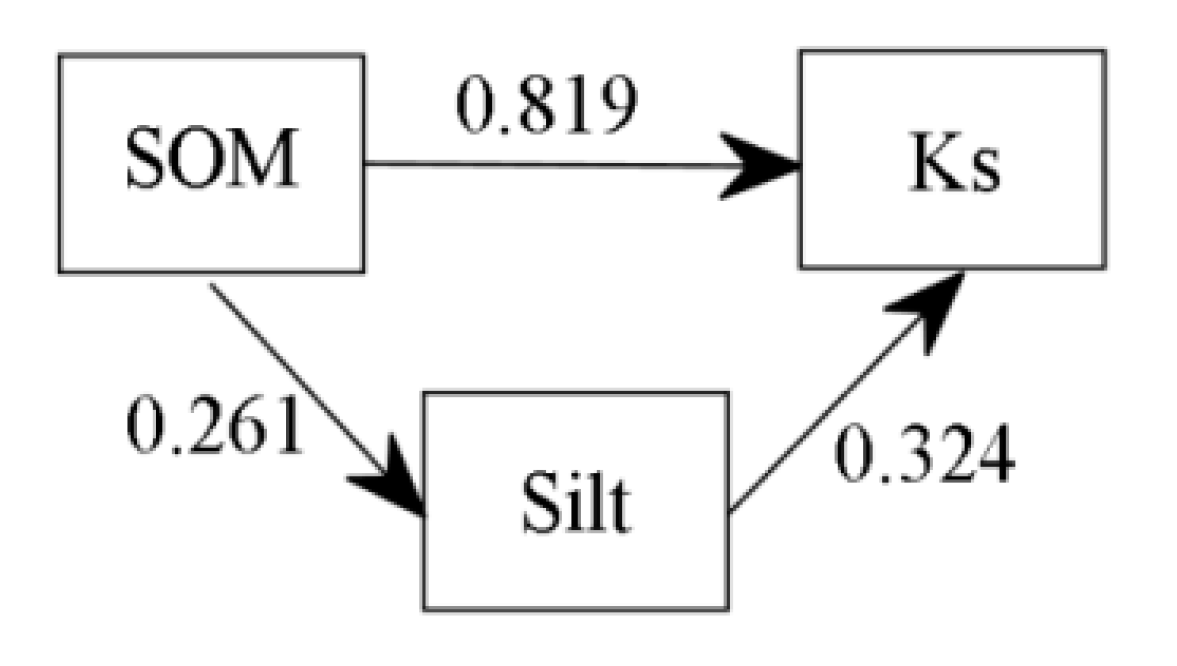
3.3. Relationship between Soil Properties and K_S

Table 4. Pearson’s correlation coefficients among soil properties.

Index	FWC	WWC	AWC	θS	α	n	TP	CP	NCP	BD	SOM	Sand	Silt	Clay
KS	0.20	0.20	0.10	0.13	−0.29	−0.11	0.88 **	0.64 **	0.50 *	−0.91 **	0.90 **	−0.13	0.54 *	−0.13
FWC	1	0.96 **	0.71 **	0.98 **	−0.79 **	−0.54 *	0.27	0.67 **	−0.54 *	−0.30	0.15	−0.71 **	0.48	0.63 *
WWC		1	0.48	0.91 **	−0.81 **	−0.74 **	0.27	0.71 **	−0.59 *	−0.30	0.11	−0.76 **	0.45	0.71 **
AWC			1	0.77 **	−0.43	0.16	0.18	0.32	−0.18	−0.19	0.20	−0.30	0.36	0.18
θS				1	−0.66 **	−0.50	0.18	0.56 *	−0.51	−0.21	0.12	−0.66 **	0.40	0.60 *
α					1	0.39	−0.41	−0.75 **	0.44	0.40	−0.14	0.68 **	−0.61 *	−0.53 *
n						1	−0.09	−0.47	0.54 *	0.12	0.05	0.57 *	−0.16	−0.62 *
TP							1	0.78 **	0.50 *	−0.99 **	0.80 **	−0.35	0.65 **	0.10
CP								1	−0.15	−0.80 **	0.47 *	−0.65 **	0.64 **	0.50 *
NCP									1	−0.47	0.61 **	0.35	0.14	−0.54 *
BD										1	−0.84 **	0.31	−0.59 **	−0.08
SOM											1	0.11	0.26	−0.30
Sand												1	−0.73 **	−0.93 **
Silt													1	0.41
Clay														1

α indicates scaling parameters related to the inverse of the air entry pressure, n indicates curve-shape parameters related to pore size distribution and θ_S indicates the saturated water content. Abbreviations: K_S, saturated hydraulic conductivity; FWC, field water content; WWC, wilting water content; AWC, available water content; TP, total porosity; CP, capillary porosity; NCP, noncapillary porosity; BD, bulk density; SOM, soil organic matter; ** p < 0.01; * p < 0.05.

shows the relationship between different soil properties. The soil water-holding characteristics of the above three forests were mainly affected by pore distribution and texture. The K_S was closely related to the soil porosity, silt content, BD and SOM. Furthermore, the absolute value of the correlation coefficients showed a decreasing sequence of BD (0.905) > SOM (0.904) >TP (0.878) > CP (0.638) > silt (0.538) > NCP (0.504). Due to the strong interaction between soil properties, multiple stepwise regression analysis was used to select the optimal factors that influenced the K_S. Eight factors, sand (X₁), silt (X₂), clay (X₃), BD (X₄), TP (X₅), CP (X₆), NCP (X₇), and SOM (X₈), were taken as the independent variable factors, and K_S was the dependent variable Y. When the independent variable factors silt (X₂) and SOM (X₈) were included, the model had the highest coefficient of determination (R²) of 0.92, which was statistically significant. The regression equation was expressed as:

$$Y=-1.029+0.031X_2+0.026X_8$$

(7)

where Y denotes K_S (mm/min).

This indicated that SOM and silt contents were the main drivers of K_S in this study area. To determine the direct and indirect effects of the above two soil properties on K_S, the path analysis method was further used for analysis. The residual path coefficient was 0.28, and the Durbin Watson statistic was 1.16, indicating that the result of path analysis was reliable. As shown in Figure 7, the direct path coefficient of SOM (0.82) for K_S was greater than that of the silt content (0.32), while the indirect path coefficient of SOM for K_S based on the silt content was 0.08.

4. Discussion

Soil development is closely related with topography, parent rock, vegetation, climate, and time [39]. The three undisturbed forests mentioned above are similar in topography and elevation, and the soil all develop on the same parent rock [28,40], so the difference in soil properties have mainly been affected by the biome [31]. Along with the process of natural vegetation restoration, the SOM content significantly increased, which has been confirmed by a large number of studies [6,15,41]. The SOM of forests mainly derives from litterfall input, and the accumulation of SOM is beneficial to the improvement of the soil physical structure [11,42,43]. The increase in SOM promotes microbial activity and the growth of the root system. The physical interpenetration of root growth is conducive to the development of soil pores, and the chemical conditions created by the exudation of organic acids by roots and microorganisms promote the decomposition of soil particles, which ultimately lead to a decrease in BD [44,45]. Along the soil profile, the BD of surface soil in different forests was significantly lower than that of other soil layers. A possible explanation for this was that the large amount of organic matter from decomposing litter first returned to the surface layer, and the improvement in the surface soil structure was the strongest. In the deep layer, the SOM decreased greatly, and the soil compaction caused by deep root growth increased the BD [10].

In this study, soil particles developed towards fine grains during the forest recovery process, consistent with the results of Błońska et al. [7] and Oktavia et al. [46]. It was worth noting that the clay content of soil in BF was similar to that in MF. The alternation of dry and wet seasons here was beneficial to the leaching of soil colloids, which drove the migration of clay particles from topsoils to deep soils. Soil particle composition was one of the main factors that determined the soil pore structure. Analysis data showed that the CP was significantly correlated with all soil particles in this area. Moreover, the CP decreased with deeper soil layers in different forests, which might also be related to the variation trend of SOM along the soil profile. The increase in SOM was conducive to soil agglomeration, which promoted soil pore formation [11]. Generally, the transformation of the soil structure would affect the soil water-holding capacity, and then the soil moisture condition changes. The soil water-holding capacity was highly correlated with the clay particles, and could be indicated by the parameter α in the VG model [47]. In this study, the correlation coefficient between CP, clay and the α value was 0.75 (p < 0.01) and 0.53 (p < 0.05), respectively. The improvement of the local soil water-holding capacity was mainly realized by the increasing quantity of clay particles and CP. It could be seen from the water-holding characteristics between forests that the water storage potential of the middle- and late-recovery-stage forests increased significantly, providing a stable water environment for vegetation growth. A good soil moisture environment might be one of the important factors promoting vegetation development in this area. Overall, vegetation restoration significantly improved the soil water storage capacity and stable soil water supply capacity, which was also reported by Owuor et al. [3] and Li et al. [42].

Vegetation restoration also gradually increased the K_S, which was consistent with the research results of Hassler et al. [48], Leite et al. [1] and Li et al. [42]. The SOM and silt particles were the main factors that affected K_S in this region, and the direct effect of SOM on K_S was the strongest. Zema et al. also reported that the SOM was one of the key parameters in driving the soil hydraulic characteristics of pure even-aged Spanish black pine stands [6]. In general, SOM affected the hydraulic properties by improving the quality of the soil colloids, and the condition and volume of soil pores played a controlling role in water permeability [47,49,50]. A study by Hao et al. showed that K_S was mainly affected by soil porosity and water-stable aggregates in subtropical forests [51]. In this study, the correlation coefficient between TP and K_S was 0.878 at a significant level. We assumed that the SOM content were conducive to the reduction of BD and thereby had an effect on K_S by increasing the soil porosity. Except for the surface layer, the K_S of MF in the other soil layers was higher than that of PF, but the difference was not significant, which might be related to the gradual decrease of SOM content below the surface layer of MF. A low organic matter content beneath the surface soil led to poor stability of the soil structure and high dispersion of soil particles, easily forming a dense and thick shell during water flow [41,52]. In addition, the proportion of CP in MF was the highest among forests, and the clay particles gradually moved down and blocked the pores in the process of water flow, which greatly weakened the permeability of the soil [10,53].

The improvement of the K_S reduced surface runoff and erosion, thus effectively replenishing soil moisture and groundwater resources [3,6]. It could be seen from Figure 8 that the accumulation rate of SOM was fast before the middle recovery stage and then slowed down. The K_S increased with the increase in SOM, and the relationship of them could be fitted by a linear function ($y=-0.149+0.029x$, R² = 0.815). We could predict that the regional eco-hydrological benefits will gradually improve with the maturation of the stands planted in Guangdong in 1980s, which is of positive significance for the response to the extreme precipitation pattern in the future [21].

Overall, vegetation restoration had significant effects on the amelioration of soil quality. The increase amount of litter return played an important role in leading to such a change. Thus, more efforts should be taken to protect the forest litter. Furthermore, the transformation of soil hydraulic performance by vegetation depended on the change in soil depth. For surface soil layer, the soil water-holding capacity and K_S improved obviously when the vegetation was restored to the middle stage. Therefore, the form of mixed forests should be further emphasized in future afforestation practice in order to improve the eco-hydrological benefits in South China.

5. Conclusions

Vegetation restoration has continuously improved the soil physicochemical properties and hydraulic characteristics in South China. The continuous accumulation of SOM has decreased the bulk density and improved the total porosity and soil hydraulic properties. The clay content and capillary porosity of soil in the middle- and late-recovery-stage forests were significantly higher than those in the early stage, which was consistent with the soil water-holding capacity. The K_S values of BF were always significantly higher than those of the other forests. In the whole soil profile, the water-holding capacity and K_S in the topsoil (above 30 cm depth) were significantly higher than those in the deep soil. Further analyses indicated that the SOM was the main driver of K_S, and the relationship of them could be fitted by a linear equation. Overall, vegetation restoration gradually ameliorated the soil hydraulic properties alongside soil structural improvement, especially the surface layer. The SOM played a key role in improving soil quality in South China. The results of the study could provide sufficient strategies for eco-environment rehabilitation and forest management.

References

1. Leite, P.A.M.; de Souza, E.S.; Dos Santos, E.S.; Gomes, R.J.; Cantalice, J.R.; Wilcox, B.P. The influence of forest regrowth on soil hydraulic properties and erosion in a semiarid region of Brazil. Ecohydrology 2018, 11, e1910. [Google Scholar] [CrossRef]
2. Saha, R.; Tomar, J.M.S.; Ghosh, P.K. Evaluation and selection of multipurpose tree for improving soil hydro-physical behaviour under hilly eco-system of North East India. Agrofor. Syst. 2007, 69, 239–247. [Google Scholar] [CrossRef]
3. Owuor, S.O.; Butterbach-Bahl, K.; Guzha, A.C.; Jacobs, S.; Merbold, L.; Rufino, M.C.; Pelster, D.E.; Díaz-Pinés, E.; Breuer, L. Conversion of natural forest results in a significant degradation of soil hydraulic properties in the highlands of Kenya. Soil Till Res. 2018, 176, 36–44. [Google Scholar] [CrossRef] [Green Version]
4. Venkatesh, B.; Lakshman, N.; Purandara, B.K.; Reddy, V.B. Analysis of observed soil moisture patterns under different land covers in Western Ghats, India. J. Hydrol. 2011, 397, 281–294. [Google Scholar] [CrossRef]
5. Gwenzi, W.; Hinz, C.; Holmes, K.W.; Phillips, I.R.; Mullins, I.J. Field-scale spatial variability of saturated hydraulic conductivity on a recently constructed artificial ecosystem. Geoderma 2011, 166, 43–56. [Google Scholar] [CrossRef]
6. Zema, D.A.; Plaza-Alvarez, P.A.; Xu, X.; Carra, B.G.; Lucas-Borja, M.E. Influence of forest stand age on soil water repellency and hydraulic conductivity in the Mediterranean environment. Sci. Total Environ. 2020, 753, 142006. [Google Scholar] [CrossRef]
7. Błońska, E.; Lasota, J.; Zwydak, M.; Klamerus-Iwan, A.; Gołąb, J. Restoration of forest soil and vegetation 15 years after landslides in a lower zone of mountains in temperate climates. Ecol. Eng. 2016, 97, 503–515. [Google Scholar] [CrossRef]
8. Chirino, E.; Bonet, A.; Bellot, J.; Sánchez, J.R. Effects of 30-year-old Aleppo pine plantations on runoff, soil erosion, and plant diversity in a semi-arid landscape in South Eastern Spain. Catena 2006, 65, 19–29. [Google Scholar] [CrossRef]
9. Neris, J.; Jimenez, C.; Fuentes, J.; Morillas, G.; Tejedor, M. Vegetation and land-use effects on soil properties and water infiltration of Andisols in Tenerife (Canary Islands, Spain). Catena 2012, 98, 55–62. [Google Scholar] [CrossRef]
10. Li, H.Q.; Liao, X.L.; Zhu, H.S.; Wei, X.R.; Shao, M.A. Soil physical and hydraulic properties under different land uses in the black soil region of Northeast China. Can. J. Soil Sci. 2019, 99, 406–419. [Google Scholar] [CrossRef]
11. Van Hall, R.L.; Cammeraat, L.H.; Keesstra, S.; Zorn, M. Impact of secondary vegetation succession on soil quality in a humid Mediterranean landscape. Catena 2017, 149, 836–843. [Google Scholar] [CrossRef]
12. Li, W.; Yan, M.; Zhang, F.Q.; Jia, Z.K. Effects of vegetation restoration on soil physical properties in the Wind-Water erosion region of the Northern Loess Plateau of China. CLEAN Soil Air Water 2012, 40, 7–15. [Google Scholar] [CrossRef]
13. Nunes, F.S.M.; Soaresfilho, B.; Rajao, R.; Merry, F. Enabling large-scale forest restoration in Minas Gerais state, Brazil. Environ. Res. Lett. 2017, 12, 44022. [Google Scholar] [CrossRef]
14. Stromberg, J.C. Restoration of riparian vegetation in the South-Western United States: Importance of flow regimes and fluvial dynamism. J. Arid Environ. 2001, 49, 17–34. [Google Scholar] [CrossRef] [Green Version]
15. Li, Y.L.; Yang, F.F.; Ou, Y.X.; Zhang, D.Q.; Liu, J.X.; Chu, G.W.; Zhang, Y.R.; Otieno, D.; Zhou, G.Y. Changes in forest soil properties in different successional stages in lower tropical China. PLoS ONE 2013, 8, e81359. [Google Scholar] [CrossRef]
16. Leung, A.K.; Garg, A.; Coo, J.L.; Ng, C.W.W.; Hau, B.C.H. Effects of the roots of Cynodon dactylon and Schefflera heptaphylla on water infiltration rate and soil hydraulic conductivity. Hydrol. Process. 2015, 29, 3342–3354. [Google Scholar] [CrossRef] [Green Version]
17. He, L.L.; Ivanov, V.Y.; Bohrer, G.; Thomsen, J.E.; Vogel, C.S.; Moghaddam, M. Temporal dynamics of soil moisture in a northern temperate mixed successional forest after a prescribed intermediate disturbance. Agric. For. Meteorol. 2013, 180, 22–33. [Google Scholar] [CrossRef]
18. Chen, X.Z.; Liu, X.D.; Zhou, G.Y.; Han, L.S.; Liu, W.; Liao, J.S. 50-Year evapotranspiration declining and potential causations in subtropical Guangdong province, Southern China. Catena 2015, 128, 185–194. [Google Scholar] [CrossRef]
19. Liu, X.D.; Sun, G.; Mitra, B.; Noormets, A.; Gavazzi, M.J.; Domec, J.; Hallema, D.W.; Li, J.Y.; Fang, Y.; King, J.S.; et al. Drought and thinning have limited impacts on evapotranspiration in a managed pine plantation on the Southeastern United States coastal plain. Agric. For. Meteorol. 2018, 262, 14–23. [Google Scholar] [CrossRef]
20. Vose, J.M.; Sun, G.; Ford, C.R.; Bredemeier, M.; Otsuki, K.; Wei, X.H.; Zhang, Z.Q.; Zhang, L. Forest ecohydrological research in the 21st century: What are the critical needs? Ecohydrology 2011, 4, 146–158. [Google Scholar] [CrossRef]
21. Zhou, G.Y.; Wei, X.H.; Wu, Y.P.; Liu, S.G.; Huang, Y.H.; Yan, J.H.; Zhang, D.Q.; Zhang, Q.M.; Liu, J.X.; Meng, Z.; et al. Quantifying the hydrological responses to climate change in an intact forested small watershed in Southern China. Glob. Chang. Biol. 2011, 17, 3736–3746. [Google Scholar] [CrossRef]
22. Cao, S.X.; Sun, G.; Zhang, Z.Q.; Chen, L.D.; Feng, Q.; Fu, B.J.; McNulty, S.; Shankman, D.; Tang, J.W.; Wang, Y.H.; et al. Greening china naturally. Ambio 2011, 40, 828–831. [Google Scholar] [CrossRef] [PubMed] [Green Version]
23. Sun, G.; Zhou, G.Y.; Zhang, Z.Q.; Wei, X.H.; McNulty, S.G.; Vose, J.M. Potential water yield reduction due to forestation across China. J. Hydrol. 2006, 328, 548–558. [Google Scholar] [CrossRef]
24. Piao, S.L.; Fang, J.Y.; Ciais, P.; Peylin, P.; Huang, Y.; Sitch, S.; Wang, T. The carbon balance of terrestrial ecosystems in China. Nature 2009, 458, 1009–1013. [Google Scholar] [CrossRef]
25. Wang, Y.D.; Wang, H.M.; Xu, M.J.; Ma, Z.Q.; Wang, Z.L. Soil organic carbon stocks and CO2 effluxes of native and exotic pine plantations in subtropical China. Catena 2015, 128, 167–173. [Google Scholar] [CrossRef]
26. Yan, J.H.; Zhou, G.Y.; Zhang, D.Q.; Chu, G.W. Changes of soil water, organic matter, and exchangeable cations along a forest successional gradient in Southern China. Pedosphere 2007, 17, 397–405. [Google Scholar] [CrossRef]
27. Zhou, G.Y.; Peng, C.H.; Li, Y.L.; Liu, S.Z.; Zhang, Q.M.; Tang, X.L.; Liu, J.X.; Yan, J.H.; Zhang, D.Q.; Chu, G.W. A climate change-induced threat to the ecological resilience of a subtropical monsoon evergreen broad-leaved forest in Southern China. Glob. Chang. Biol. 2013, 19, 1197–1210. [Google Scholar] [CrossRef]
28. Huang, Y.H.; Li, Y.L.; Xiao, Y.; Wenigmann, K.O.; Zhou, G.Y.; Zhang, D.Q.; Wenigmann, M.; Tang, X.L.; Liu, J.X. Controls of litter quality on the carbon sink in soils through partitioning the products of decomposing litter in a forest succession series in South China. For. Ecol. Manag. 2011, 261, 1170–1177. [Google Scholar] [CrossRef]
29. Zhou, G.Y.; Liu, S.G.; Li, Z.A.; Zhang, D.Q.; Tang, X.L.; Zhou, C.Y.; Yan, J.H.; Mo, J.M. Old-growth forests can accumulate carbon in soils. Science 2006, 314, 1417. [Google Scholar] [CrossRef] [Green Version]
30. Liu, X.D.; Chen, X.Z.; Li, R.H.; Long, F.L.; Zhang, L.; Zhang, Q.M.; Li, J.Y. Water-use efficiency of an old-growth forest in lower subtropical China. Sci. Rep. 2017, 7, 42761. [Google Scholar] [CrossRef]
31. Yan, J.H.; Zhou, G.Y.; Chen, Z.Y. Coupling study on soil structure and hydrological effects for three succession communities in Dinghushan. Res. Trends Resour. Ecol. Environ. Netw. 2000, 11, 6–11. (In Chinese) [Google Scholar]
32. Buol, S.W.A.; Southard, R.J.B.; Graham, R.C.C.; McDaniel, P.A.D. Soil Genesis and Classification, 5th ed.; Iowa State Press: Iowa City, IA, USA, 2003; pp. 339–347. [Google Scholar]
33. Peng, S.L.; Wang, B.S. Forest succession at Dinghushan, Guangdong, China. Bot. J. South China 1993, 1, 34–42. [Google Scholar]
34. Tian, J.; Zhang, B.Q.; He, C.S.; Yang, L.X. Variability in soil hydraulic conductivity and soil hydrological response under different land covers in the mountainous area of the Heihe river watershed, Northwest China. Land Degrad. Dev. 2016, 28, 1437–1449. [Google Scholar] [CrossRef]
35. ASTM D891-18, Standard Test Methods for Specific Gravity, Apparent, of Liquid Industrial Chemicals; ASTM International: West Conshohocken, PA, USA, 2018; Available online: www.astm.org (accessed on 20 September 2019).
36. Gaudette, H.E.; Flight, W.R.; Toner, L.; Folger, D.W. An inexpensive titration method for the determination of organic carbon in recent sediments. J. Sediment. Petrol. 1974, 44, 249–253. [Google Scholar] [CrossRef]
37. Shwetha, P.; Varija, K. Soil water retention curve from saturated hydraulic conductivity for sandy loam and loamy sand textured soils. Aquat. Procedia 2015, 4, 1142–1149. [Google Scholar] [CrossRef]
38. Van Genuchten, M.T. A closed-form equation for predicting the hydraulic conductivity of unsaturated soils. Soil Sci. Soc. Am. J. 1980, 44, 892–898. [Google Scholar] [CrossRef] [Green Version]
39. Huggett, R.J. Soil chronosequences, soil development, and soil evolution: A critical review. Catena 1998, 32, 155–172. [Google Scholar] [CrossRef]
40. Shen, C.D.; Yi, W.X.; Sun, Y.M.; Xing, C.P.; Yang, Y.; Chao, Y.; Li, Z.A.; Peng, S.L.; An, Z.S.; Liu, T.S. Distribution of C−14 and C−13 in forest soils of the Dinghushan Biosphere Reserve. In Proceedings of the 17th International Radiocarbon Conference, Jerusalem, Israel, 18–23 June 2000. [Google Scholar]
41. Gu, C.J.; Mu, X.M.; Gao, P.; Zhao, G.J.; Sun, W.Y.; Tatarko, J.; Tan, X.J. Influence of vegetation restoration on soil physical properties in the Loess Plateau, China. J. Soil Sediments 2019, 19, 716–728. [Google Scholar] [CrossRef]
42. Li, Y.Y.; Shao, M.A. Change of soil physical properties under long-term natural vegetation restoration in the Loess Plateau of China. J. Arid Environ. 2006, 64, 77–96. [Google Scholar] [CrossRef]
43. Piaszczyk, W.; Lasota, J.; Błońska, E. Effect of organic matter released from deadwood at different decomposition stages on physical properties of forest soil. Forests 2020, 11, 24. [Google Scholar] [CrossRef] [Green Version]
44. Marschner, P.; Crowley, D.; Rengel, Z. Rhizosphere interactions between microorganisms and plants govern iron and phosphorus acquisition along the root axis–model and research methods. Soil Biol. Biochem. 2011, 43, 883–894. [Google Scholar] [CrossRef]
45. Pastore, G.; Kaiser, K.; Kernchen, S.; Spohn, M. Microbial release of apatite- and goethite-bound phosphate in acidic forest soils. Geoderma 2020, 370, 114360. [Google Scholar] [CrossRef]
46. Oktavia, D.; Setiadi, Y.; Hilwan, I. The comparison of soil properties in heath forest and post-tin mined land: Basic for ecosystem restoration. Procedia Environ. Sci. 2015, 28, 124–131. [Google Scholar] [CrossRef] [Green Version]
47. Bittelli, M.A.; Campbell, G.S.B.; Tomei, F.C. Soil Physics with Python: Transport in the Soil-Plant-Atmosphere System; Oxford University Press: Oxford, UK, 2015; pp. 26–32. [Google Scholar]
48. Hassler, S.K.; Zimmermann, B.; van Breugel, M.; Hall, J.S.; Elsenbeer, H. Recovery of saturated hydraulic conductivity under secondary succession on former pasture in the humid tropics. For. Ecol. Manag. 2011, 261, 1634–1642. [Google Scholar] [CrossRef]
49. Aimrun, W.; Amin, M.S.M.; Eltaib, S.M. Effective porosity of paddy soils as an estimation of its saturated hydraulic conductivity. Geoderma 2004, 121, 197–203. [Google Scholar] [CrossRef]
50. Jarvis, N.J. A review of non-equilibrium water flow and solute transport in soil macropores: Principles, controlling factors and consequences for water quality. Eur. J. Soil Sci. 2007, 58, 523–546. [Google Scholar] [CrossRef]
51. Hao, M.Z.; Zhang, J.C.; Meng, M.J.; Chen, H.Y.H.; Guo, X.P.; Liu, S.L.; Ye, L.X. Impacts of changes in vegetation on saturated hydraulic conductivity of soil in subtropical forests. Sci. Rep. 2019, 9, 8372–8379. [Google Scholar] [CrossRef] [Green Version]
52. Lado, M.; Paz, A.; Benhur, M. Organic matter and aggregate size interactions in infiltration, seal formation, and soil loss. Soil Sci. Soc. Am. J. 2004, 68, 935–942. [Google Scholar] [CrossRef]
53. Lado, M.; Paz, A.; Benhur, M. Organic matter and aggregate-size interactions in saturated hydraulic conductivity. Soil Sci. Soc. Am. J. 2004, 68, 234–242. [Google Scholar] [CrossRef]
Figure 1. Location of the experimental sites in Dinghushan Biosphere Reserve (c), Zhaoqing (b), Guangdong, China (a). Abbreviations: OLT, other land-use types; PF, Pinus massoniana forest; MF, mixed Pinus massoniana/broad-leaved forest; BF, monsoon evergreen broad-leaved forest.
Forests 11 01111 g001
Figure 2. Soil organic matter (a) and bulk density (b) of the 0–90 cm soil layer of different forests. Values are the means ± SE. Lowercase letters above the columns represent statistically significant differences among stand types for the same soil layer (Duncan’s test, p < 0.05). Abbreviations: SOM, soil organic matter; BD, bulk density; PF, Pinus massoniana forest; MF, mixed Pinus massoniana/broad-leaved forest; BF, monsoon evergreen broad-leaved forest.
Forests 11 01111 g002
Figure 3. Soil mechanical composition including sand (a), silt (b), and clay (c) contents of the 0–90 cm soil layer of the different forests. Values are the means ± SE. Lowercase letters above the columns represent statistically significant differences among stand types for the same soil layer (Duncan’s test, p < 0.05). Abbreviations: PF, Pinus massoniana forest; MF, mixed Pinus massoniana/broad-leaved forest; BF, monsoon evergreen broad-leaved forest.
Forests 11 01111 g003
Figure 4. Soil porosity distribution of the 0–90 cm soil layer of BF (a), MF (b) and PF (c). Abbreviations: TP, total porosity; CP, capillary porosity; NCP, noncapillary porosity; PF, Pinus massoniana forest; MF, mixed Pinus massoniana/broad-leaved forest; BF, monsoon evergreen broad-leaved forest.
Forests 11 01111 g004
Figure 5. Soil water retention curves at depths of 0–10 cm (a), 10–20 cm (b), 20–40 cm (c), 40–60 cm (d), and 60–100 cm (e) in the three forests. Abbreviations: PF, Pinus massoniana forest; MF, mixed Pinus massoniana/broad-leaved forest; BF, monsoon evergreen broad-leaved forest.
Forests 11 01111 g005
Figure 6. Distribution of KS along the soil profile (a) and the differences in average KS in the different forests (b) in Dinghushan. Values are the means ± SE. Lowercase letters above the columns represent statistically significant differences among stand types (Duncan’s test, p < 0.05). Abbreviations: KS, saturated hydraulic conductivity; PF, Pinus massoniana forest; MF, mixed Pinus massoniana/broad-leaved forest; BF, monsoon evergreen broad-leaved forest.
Forests 11 01111 g006
Figure 7. Path diagram for the relationship between KS and the main effective soil properties. The magnitude of the numerical values in the figure indicates the level of effects between the factors. Abbreviations: KS, saturated hydraulic conductivity; SOM, soil organic matter.
Forests 11 01111 g007
Figure 8. The variation trend of average SOM content across the 0–90 depth with vegetation restoration time (a) and the relationship between the SOM and KS (b). Abbreviations: SOM, soil organic matter; KS, saturated hydraulic conductivity.
Forests 11 01111 g008