Estimation of DBH at Forest Stand Level Based on Multi-Parameters and Generalized Regression Neural Network

Abstract

The diameter at breast height (DBH) is an important factor used to estimate important forestry indices like forest growing stock, basal area, biomass, and carbon stock. The traditional DBH ground surveys are time-consuming, labor-intensive, and expensive. To reduce the traditional ground surveys, this study focused on the prediction of unknown DBH in forest stands using existing measured data. As a comparison, the tree age was first used as the only independent variable in establishing 13 kinds of empirical models to fit the relationship between the age and DBH of the forest subcompartments and predict DBH growth. Second, the initial independent variables were extended to 19 parameters, including 8 ecological and biological factors and 11 remote sensing factors. By introducing the Spearman correlation analysis, the independent variable parameters were dimension-reduced to satisfy very significant conditions (p ≤ 0.01) and a relatively large correlation coefficient (r ≥ 0.1). Finally, the remaining independent variables were involved in the modeling and prediction of DBH using a multivariate linear regression (MLR) model and generalized regression neural network (GRNN) model. The (root-mean-squared errors) RMSEs of MLR and GRNN were 1.9976 cm and 1.9655 cm, respectively, and the R² were 0.6459 and 0.6574 respectively, which were much better than the values for the 13 traditional empirical age–DBH models. The use of comprehensive factors is beneficial to improving the prediction accuracy of both the MLR and GRNN models. Regardless of whether remote sensing image factors were included, the experimental results produced by GRNN were better than MLR. By synthetically introducing ecological, biological, and remote sensing factors, GRNN produced the best results with 1.4688 cm in mean absolute error (MAE), 13.78% in MAPE, 1.9655 cm for the RMSE, 0.6574 for the R², and 0.0810 for the Theil’s inequality coefficient (TIC), respectively. For modeling and prediction based on more complex tree species and a wider range of samples, GRNN is a desirable model with strong generalizability.

1. Introduction

In forest monitoring, the diameter at breast height (DBH) is the diameter of a cross-section of a tree trunk 1.3 m above the ground. The DBH is an important factor used to estimate important forestry indices like forest growing stock, basal area, biomass, and carbon stock. The traditional DBH ground surveys effectively provide objective and reliable monitoring and managing information for forest resources [1,2,3,4], but they are time-consuming, labor-intensive, expensive, and hard to implement, particularly in mountainous and forest areas [4].

The establishment of DBH prediction models has mainly been based on stand growth models. Three kinds of models are frequently used: Empirical models, process models, and hybrid models [5]. Empirical models require some biological factors such as tree height, age, and crown width as independent variable sets, and introduce some regression estimation methods, such as curve, Gompertz, Schumacher, or Richards models, in estimating DBH [6,7,8,9,10]. Although their construction is intuitive and simple, the variability of the empirical relationship between the dependent and independent variables means the empirical models are less adaptable. By introducing physiological and ecological factors, such as climate, precipitation, and soil, the process models improve the ability to simulate stand growth [11]. The inclusion of many physiological and ecological factors produces highly complex and inflexible process models, which leads to difficulties in meeting the actual requirements. In combining empirical models and process models, hybrid models—which include the linear mixed effect model and the nonlinear mixed effect model—have better estimation accuracy and adaptability. However, the combination further increases the complexity and flexibility of the models.

Artificial neural networks (ANNs) can be effectively used to solve nonlinear problems [12], such as the prediction of forest growth. To find more effective methods for forest growth estimation, many experts and scholars have introduced ANN models into the field of forestry for the dynamic monitoring of forest resources and the simulation of forest growth process [13,14,15]. Compared with traditional stand growth models, the backpropagation neural network (BP-NN) model provides the best prediction effect to fit and analyze the growth of tree DBH [16,17,18].

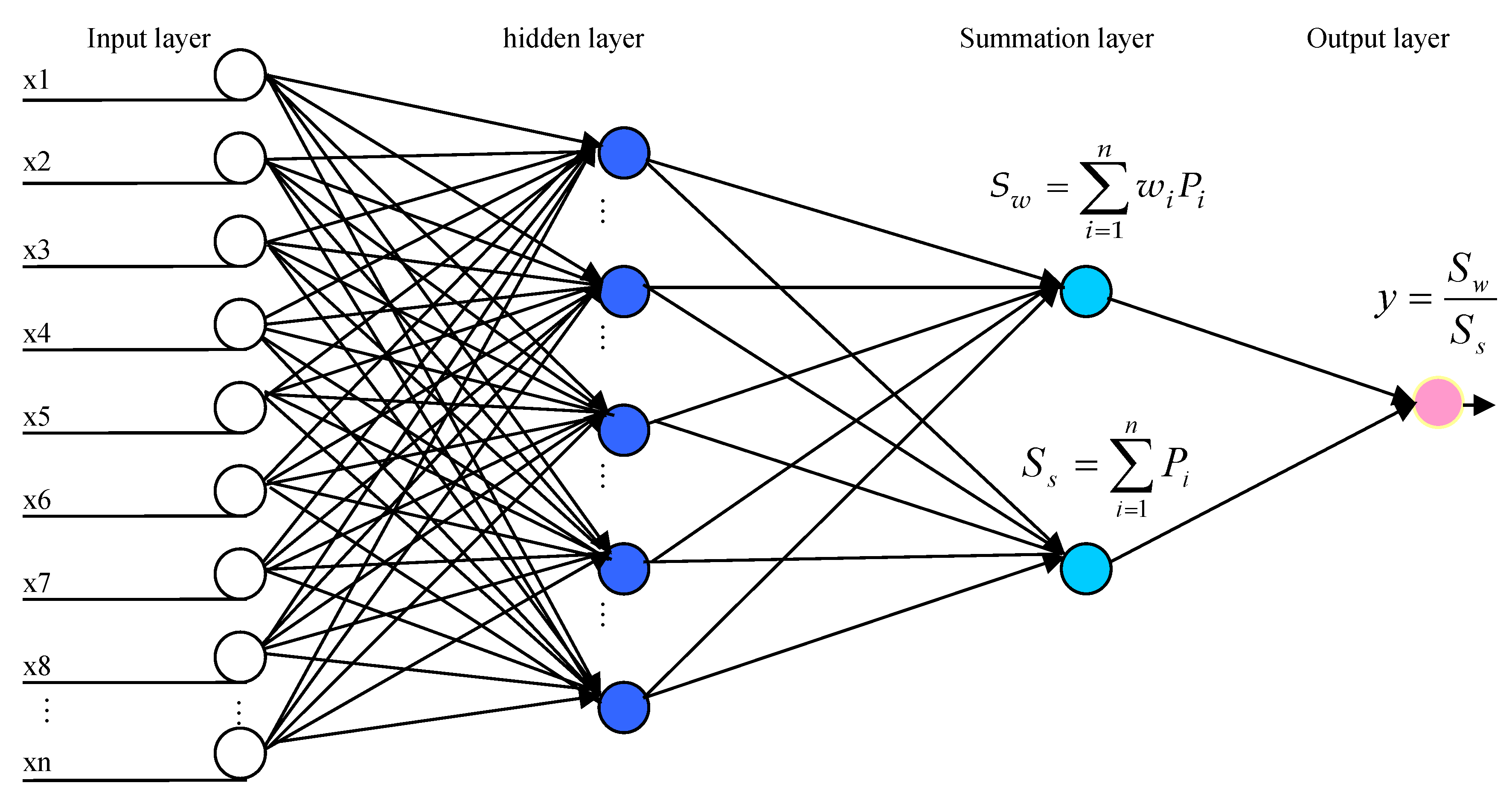
Compared with the BP-NN model, the generalized regression neural network (GRNN) model has the advantages of a simpler structure, fewer parameters, a faster prediction speed, and less computational complexity [19]. Correspondingly, some scholars have used the GRNN model to estimate forest parameters [20,21].

Scholars have found that DBH is strongly affected by environmental factors, such as topography, soil, and climate [22,23,24,25,26,27]. Pach et al. showed that at fertile mountain sites and highland forest sites, fir trees reached the highest growing stock [23]. Li et al. showed that the DBH growth of natural Korean pine forest is affected by topographic factors, particularly the elevation and slope direction [24]. Ou et al. found that DBH growth is correlated with the slope direction, soil hydrolytic nitrogen, dominant tree height, average tree height, and tree density [25]. Yu et al. and Wang et al. found that temperature and precipitation affect the DBH growth of larch, spruce, fir, and Tianshan spruce [26,27].

The increasing resolution of remote sensing images has provided additional benefits for forest monitoring. Zarco-Tejada et al. showed that the tree height can be obtained by three-dimensional (3D) reconstruction from unmanned aerial vehicle (UAV) images [28]. Ibanez et al. reported that various forest parameters, with the exception of DBH, can be directly obtained using light detection and ranging (LIDAR) images according to the point cloud characteristics at different forest levels [29]. Using field data and vegetation index (VI) data derived from Systeme Probatoire d’Observation de la Terre 5 (SPOT-5) satellite images, Muhd-Ekhzarizal et al. used some simple and multilinear regression methods to estimate the aboveground biomass in mangrove forests [30]. Chrysafis et al. found a strong correlation between the growing stock volume and three indices derived from Sentinel-2 images, i.e., the difference vegetation index (DVI), enhanced vegetation index (EVI), and perpendicular vegetation index (PVI) [31]. Using ALOS-PALSAR L-band full-polarization data, Chowdhury et al. estimated the forest growing stock volume (GSV) and showed that the GSV at forest stand level in Siberia could be quantified with reasonable accuracy, and that temporal variations of GSV could be better tracked [2]. Vegetation indices (VIs) reflect the dynamic changes of forests to some extent and are helpful in predicting forest parameters. For example, Mou et al. indicated that the normalized difference vegetation index (NDVI) is most sensitive to changes in the canopy leaf area index and Laurin et al. added NDVI values to aboveground biomass estimations to obtain better results [32,33]. Han et al. showed that the vegetation indices from different remote sensing data sources have different separability from ground objects [34]. Reyadh et al. found that a similar variability in the average derived NDVI from different remote sensing data sources, but the average derived NDVI values were different [35]. Buheaosier showed that the range of NDVIs is related to the spatial resolution of remote sensing data sources [36]. However, limited by a lack of human power, high costs, weak endurance capability, and a small communication range, UAV remote sensing and radar remote sensing are still difficult to apply to large-scale forest monitoring [37,38]. Furthermore, airborne imagery is easily affected by wind power and terrain, and is vulnerable to air traffic control [39]. In China, especially in the south regions, the weather is usually changeable, and the terrain is usually complex, hence airborne imageries are still difficult to be applied in large-scale forest monitoring. Therefore, satellite remote sensing images remain the main supplementary data resource for dynamic monitoring of large-scale forest resources in China.

During the estimation or prediction of DBH at the forest stand level, the data from the permanent plots (the basic units of national forest inventory) are frequently chosen to validate the various models [40,41]. However, in China, the number of subcompartments is much larger than the number of permanent plots. To reduce the cost of investigating, the estimation of DBH based on subcompartments is more valuable than the methods based on permanent forest plots.

This study focused on the prediction of DBH at the subcompartment’s level in Longquan city. The specific purposes of this paper are to: (1) Ascertain the suitable ecological factors, biological factors and remote sensing factors which have great impact on DBH with a relatively low cost for data-acquisition; (2) explore a more accurate and more generalizable model to predict DBH. The specific steps of this study are as follows: First, using tree age as the only independent variable, 13 kinds of empirical models were established to fit the relationship between the tree age and the DBH of forest subcompartments and predict DBH growth. Second, the independent variables were extended to 19 parameters, including 8 ecological and biological factors (elevation, slope, aspect, soil depth, humus thickness, age of tree, canopy density, and number of stems per hectare), and 11 remote sensing factors (bands 2–7 (B2–B7) from the operational land imager (OLI) sensor of the Landsat-8 satellite, NDVI, ratio vegetation index (RVI), DVI, EVI, and red index (RI)). The correlation analysis method was introduced to reduce the dimensions of the independent variables separately for either the set of ecological and biological factors or the set of remote sensing factors. Lastly, the remaining independent variables were adopted for modeling and prediction of DBH of the forest subcompartments using a multivariate linear regression (MLR) model and GRNN model.

2. Materials and Methods

2.1. Study Area

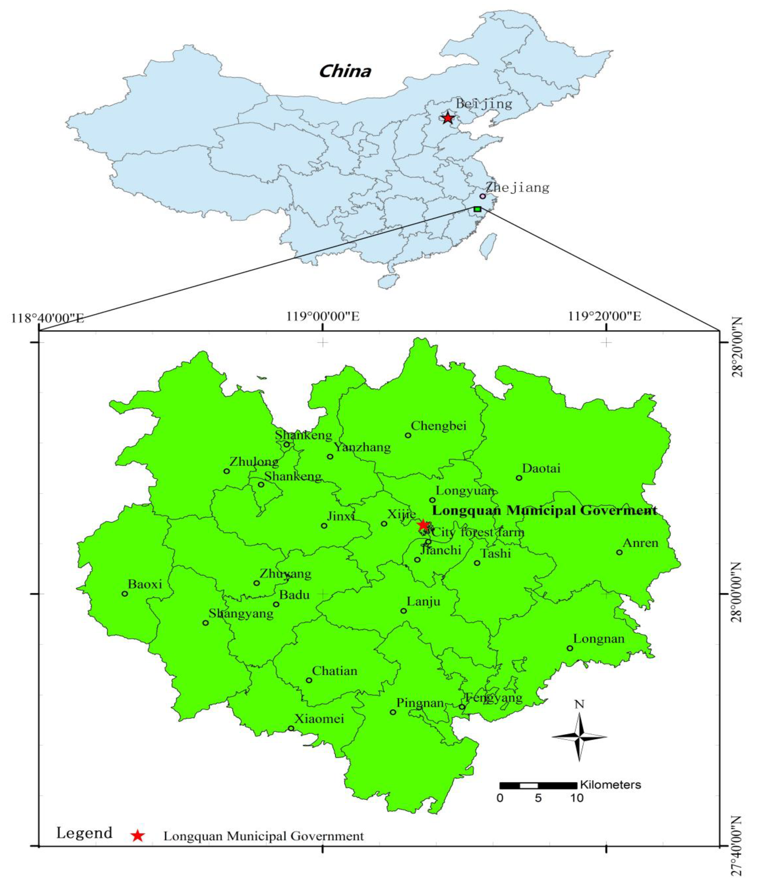
Longquan (Figure 1), as a southwest city in Zhejiang province in China, with a total area of 3059 km², extends from 118°42′ to 119°25′ E, and 27°42′ to 28°20′ N. Due to its location in a central subtropical monsoon climate zone, the city is warm and humid with abundant rainfall. Longquan is the largest forested city in Zhejiang province, with 265,667 ha of forest resources, 14.56 million cubic meters of forest growing stock, and a forest coverage of 84.2% [42].

2.2. Research Data

The research data included the inventory data for forest management planning and design, the digital elevation model (DEM), and remote sensing images from Landsat-8 Thematic Mapper (TM). The 2017 inventory data were supplied by the Forestry Bureau of Longquan. The TM and DEM data were both derived from the Geospatial Data Cloud [43].

Six factors were derived from the inventory data for forest management planning and design, including DBH, soil depth, humus thickness, canopy density, number of stems per hectare, and age of tree. Three factors, elevation, slope, and aspect, were obtained from DEM and 11 factors were derived from the remote sensing images, including B2–B7, NDVI, RVI, DVI, EVI, and RI.

The inventory data, containing 58,910 records of forest subcompartments, were obtained from the Forestry Bureau of Longquan in 2017. According to the rules for the technical operation of the inventory for forest management planning and design in Zhejiang province (2014) [44], the original inventory data acquisition procedure is as follows: Within the scope of the subcompartments, some standard plots or angle gauge plots are laid out using random, mechanical, or other sampling methods, and the corresponding forest factors are measured in the plots by professionals, and the subcompartment factors are then calculated. Therefore, whether modeling or predicting, all the data—including DBH, soil depth, humus thickness, canopy density, number of stems per hectare, and age of tree—are presented as an average value at the forest subcompartment level. The unsuitable data were removed via preliminary processing, including records for zero-volume subcompartments which were located in non-forest plots, or those with subcompartment DBHs less than 5 cm, which do not meet the standard for measurement [44]. Therefore, the final inventory data included 35,763 records of forest subcompartments. These were randomly separated into two groups, with one containing 25,000 records for modeling, and the remaining 10,763 records used as testing data for prediction (

Table 1. Diameter at breast height (DBH) and the tree age of the inventory data used for modeling and prediction.

	Modeling Data		Prediction Data
	DBH (cm)	Age (years)	DBH (cm)	Age (years)
Maximum	80	200	35	200
Minimum	5	2	5	3
Average	11.69	26.43	11.75	26.62
SD	3.48	12.07	3.35	12.07

).

The DEM data were originally obtained from the first version data of the global DEM (GDEM) generated by the advanced spaceborne thermal emission and reflection radiometer, including four images in 2009, with 30 m resolution, IMG data type, World Geodetic System 1984 (WGS84), and the universal transverse mercator (UTM) projection. The data were obtained from the International Scientific and Technical Data Mirror Site, Computer Network Information Center, Chinese Academy of Sciences [43].

The remote sensing images, which correspond fully with the timeline of the inventory data, were generated by Landsat-8 TM from Landsat satellites in 2017. There are two sensors in each Landsat satellite that collect data from discrete portions of the electromagnetic spectrum, known as bands, according to their wavelength. The Landsat-8 satellite’s images, with the UTM/WGS 84 coordinate system, include 11 bands representing portions of the electromagnetic spectrum, consisting of visible bands and invisible bands to the human eye. Here, the visible bands include 5 bands, i.e., band 1, called the coastal band, with wavelengths of 0.433–0.453 μm; band 2, called the blue band, with wavelengths of 0.450–0.515 μm; band 3, called the green band, with wavelengths of 0.525–0.600 μm; band 4, called the red band, with wavelengths of 0.630–0.680 μm; and band 8, called the pan band, with wavelengths of 0.500–0.680 μm. The invisible bands include 6 bands, i.e., band 5, called the near infrared (NIR) band, with wavelengths from 0.845 to 0.885 μm; band 6, called the SWIR-1 band, with wavelengths of 1.560–1.660 μm; band 7, called the SWIR-2 band, with wavelengths of 2.100–2.300 μm; band 9, called the cirrus band, with wavelengths of 1.360–1.390 μm; band 10, called the TIRS-1 band, with wavelengths of 10.6–11.2 μm; and band 11, called the TIRS-2 band, with wavelengths of 11.5–12.5 μm. The spatial resolution of the bands is mostly 30 m except for band 8, which contains panchromatic data with a resolution of 15 m, and bands 10 and 11 provide data collected at a 100 m resolution.

3. Methods

3.1. Data Preprocessing and Integration

The geometric correction, radiometric calibration, and atmospheric correction of Landsat-8 TM images were handled by ENVI 5.3 (Exelis Visual Information Solutions, Boulder, CO, USA). Afterwards, VI was calculated from the processed images by the band math tool in ENVI 5.3. In ArcGIS 10.2 (Environmental Systems Research Institute, Redlands, CA, USA), the DEM data and remote sensing data were extracted based on each subcompartment. For modeling and prediction, all the preprocessed data, including the inventory data for forest management planning and design, DEM data, and remote sensing images from TM, were integrated into the same relational database.

3.2. Empirical Model

The traditional models used to predict DBH of the forest subcompartment are usually based on the relationship between DBH and the independent variables of tree age, height, and crown width. However, the costs of data-acquisition of the height and crown width of the trees are quite high in practical measurement. In contrast, the tree-age of the subcompartment refers to the average tree-age of the dominant species which is usually stable in a relative short period. In this way, as long as the initial values of the tree age are obtained successfully, only 1 needs to be added for each year after the measurement. Thus, the cost of data-acquisition is relatively low. Therefore, the 13 empirical models based on the age–DBH model that use tree age as the only independent variable [45,46,47,48] were selected to predict DBH in this paper (

Table 2. The 13 empirical models based on the age—diameter at breast height (DBH) model for the prediction of DBH.

Model Name	Equation
Linear model	$y=a+bx$
Logarithmic curve model	$y=a+b\ln (x)$
Reciprocal curve model	$y=a+b/x$
Conic model	$y=a+bx+c{x}^2$
Cubic curve model	$y=a+bx+c{x}^2+d{x}^3$
Compound curve model	$y=a{b}^x$
Power function curve model	$y=a{x}^b$
S-shaped curve model	$y=\exp (a+b/x)$
Growth curve model	$y=\exp (a+bx)$
Exponential curve model	$y=a\exp (a+bx)$
Logistic curve model	$y={\left(\frac{1}{u}+a{b}^x\right)}^{-1}$
Gompertz model	$y=a\exp (-b\exp (-cx))$
Schumacher model	$y=a\exp (-b/x)$

Note: y denotes the DBH of the forest subcompartments, x is the age of tree; a, b, c, and d are the parameters to be estimated.

).

3.3. Correlation Analysis

The nonparametric test is an important part of statistical analysis methods that is used to infer the population distribution using the sample data in situations where the total variance is unknown or uncertain. As the total variance in advance was unable to be estimated, the nonparametric test was preferable for inferring the population distribution. The Spearman rank correlation analysis is a specific method used to implement the nonparametric test to estimate the correlation between two variables. Here, the observed values of two variables needed to be paired with the graded data originally or converted from the observed data of the continuous variables without considering the overall distribution pattern and sample size of the two variables. The formula for calculating the correlation coefficient of the Spearman rank is shown in Equation (1), and the calculation is based on the rank of the value, rather than the value itself. The calculation was conducted in SPSS 20 (International Business Machines Corporation, Armonk, NY, USA) using the double tail test.

$$r=\frac{{\displaystyle \sum _{i=1}^n(R_i-\overline{R})(S_i-\overline{S})}}{{\left[{\displaystyle \sum _{i=1}^n{(R_i-\overline{R})}^2{\displaystyle \sum _{i=1}^n{(S_i-\overline{S})}^2}}\right]}^{\frac{1}{2}}}$$

(1)

where R_i is the rank of the ith observed value for variable x; S_i is the rank of the ith observed value for variable y; $\overline{R}$ and $\overline{S}$ are the average ranks of variables x and y, respectively; and n denotes the total number of observed values.

3.4. Multiple Linear Regression Model

The multiple linear regression (MLR) is a statistical method. The MLR can be used to predict the values of a response variable using several explanatory variables [49] and fitting the relationship between the independent variables and dependent variable. It has been represented in Equation (2), and was implemented in SPSS 20.

$$y={\beta }_0+{\beta }_1{\mathrm{x}}_1+{\beta }_2{\mathrm{x}}_2+\cdots +{\beta }_{\mathrm{n}}\mathrm{xi}+\epsilon$$

(2)

where y denotes the dependent variable, xi denotes the ith independent variable, ${\beta }_0$ represents a constant, ${\beta }_{\mathrm{i}}$ denotes the slope coefficient for the ith explanatory variable, and $\epsilon$represents the residual.

The process for solving the parameters for Equation (2) was as follows. First, leaving aside the remote sensing parameters, the four factors (elevation, age of tree, canopy density, and the number of trees per hectare) that were involved in the MLR analysis were obtained from the inventory data for forest management planning and design or DEM data. The various MLR selection methods include the forward, backward, stepwise, entering, and deletion methods. This study chose the stepwise method, also called the stepwise regression model, to filter the independent variables to feed to the MLR model, which is represented in Equation (3). This was implemented in SPSS 20.

$$\mathrm{Y}=6.700668+0.130314{\mathrm{X}}_1-0.037245{\mathrm{X}}_2-0.000996{\mathrm{X}}_3+9.170188{\mathrm{X}}_4$$

(3)

where X₁ is the tree age, X₂ is the number of trees per hectare, X₃ denotes elevation, and X₄ is canopy density.

Subsequently, the seven remote sensing image factors (bands 2–7 and DVI) together with the previous four factors (elevation, age of tree, canopy density, and number of trees per hectare), for a total of 11 factors, were introduced into the MLR model to analyze the linear relationship among DBH and the parameters. This study also chose the stepwise regression method to fit the MLR model in SPSS 20, and the fitting equation was established as:

$$\begin{array}{c}\mathrm{Y}=7.189245+0.139459{\mathrm{X}}_1-0.036492{\mathrm{X}}_2-0.001706{\mathrm{X}}_3+8.663880{\mathrm{X}}_4+0.002292{\mathrm{X}}_5-\\ 0.005670{\mathrm{X}}_6+0.005301{\mathrm{X}}_7-0.004161{\mathrm{X}}_8-0.012977{\mathrm{X}}_9+0.020564{\mathrm{X}}_{10}\end{array}$$

(4)

where the variables from X₁ to X₄ denote tree age, number of trees per hectare, elevation, and canopy density, respectively; X₅ denotes DVI; X₆ to X₈ denote bands 2 through 4, respectively; and X₉ and X₁₀ are bands 6 and 7, respectively. Note that band 5 was removed after the execution of the stepwise regression model.

3.5. Generalized Regression Neural Network

The generalized regression neural network (GRNN) was first proposed by Specht in 1991 [50]. On the basis of the estimation of a probability distribution function, the GRNN can solve nonlinear approximative problems. The GRNN gradually converges to the optimal regression surface as the number of training samples increases. The advantages of the GRNN include its simplicity and high accuracy in modeling and prediction. The GRNN architecture includes four layers (Figure 2): Input, hidden, summation, and output [51].

In the input layer, the amount of neurons is determined by the number of the input variables, and each neuron represents an input variable. The input layer does not process the signal but nonlinearly transmits the signal to the hidden layer.

In the hidden layer, the neurons accept the information from the input layer and express the relationship (P_i) between the input layer and hidden layer with a pattern of radial basic function as the activation function. The radial basic function is usually represented by the Gaussian function:

$$P_i=\exp (-\frac{{(X-X_i)}^T(X-X_i)}{2{\sigma }^2})$$

(5)

where I = 1, 2, …, n, with n representing the number of training cases; P_i denotes the multivariate Gaussian function; σ denotes the smoothing parameter, which is also called the spread parameter; X represents the input variable; and X_i denotes a training sample for the ith neuron of the hidden layer.

There are two summations in the summation layer, S_w and S_s, which are defined by Equations (6) and (7), respectively. S_w is the weighted summation of the summation layer and S_s is the arithmetic summation of the summation layer, where w_i represents the weight of the ith neuron of the hidden layer to connect to the summation layer.

$$S_w={\displaystyle \sum _{i=1}^n{w}_i{P}_i}$$

(6)

$$S_s={\displaystyle \sum _{i=1}^n{P}_i}$$

(7)

In the output layer, the output variable y is calculated using Equation (8). The dimension of the output matrix of the final training of the neural network depends on the number of neurons.

$$y=\frac{S_w}{S_s}$$

(8)

The GRNN model was implemented in MATLAB 2017b (The MathWorks, Natick, MA, USA). Its network structure was determined by:

$$net=newgrnn(x,y,spread)$$

(9)

where x denotes the input matrix for the independent variables, y denotes the output matrix for the dependent variables, and spread is the smoothing factor. The value of this factor was tested by cross-validation.

3.6. Model Performance Metrics

The following indices can be used to assess the performance of each model, where Y_i represents the measured values, y_i represents the predicted values for sample i, $\overline{Y}$ denotes the predicted mean, $\overline{y}$ denotes the observed mean, and n denotes the total number of samples.

The first statistical metric is the mean absolute error (MAE), expressed by

$$MAE=\frac{1}{n}\left|{\displaystyle \sum _{i=1}^n(Y_i-y_i})\right|$$

(10)

The mean absolute percentage error (MAPE) is represented by

$$MAPE=\frac{1}{n}{\displaystyle \sum _{i=1}^n\frac{\left|Y_i-y_i\right|}{\left|Y_i\right|}}\times 100\%$$

(11)

The root-mean-squared error (RMSE), one of the most commonly used indicators for evaluating performance, is expressed by

$$RMSE=\sqrt{\frac{1}{n}{\displaystyle \sum _{i=1}^n{(Y_i-y_i)}^2}}$$

(12)

The coefficient of determination (R²) is a statistical index used to describe the degree to which a change in the results can be explained by a change in the independent variables. R² ranges from 0 to 1; the closer R² is to 1, the better the model effect. The values of R² are calculated by:

$$R^2=\frac{{\left[{\displaystyle \sum _{i=1}^n(Y_i-\overline{Y})(y_i-\overline{y})}\right]}^2}{{\displaystyle \sum _{i=1}^n{(Y_i-\overline{Y})}^2\text{•}{\displaystyle \sum _{i=1}^n{(y_i-\overline{y})}^2}}}$$

(13)

The Theil’s inequality coefficient (TIC) is a measure of the difference between the measured and predicted values. When the value is between 0 and 1, and the closer the value is to 0, the better the prediction effect. The TIC represented by:

$$TIC=\frac{\sqrt{\frac{1}{n}{\displaystyle \sum _{i=1}^n{(Y_i-y_i)}^2}}}{\sqrt{\frac{1}{n}{\displaystyle \sum _{i=1}^n{Y}_i{}^2}}+\sqrt{\frac{1}{n}{\displaystyle \sum _{i=1}^n{y}_i{}^2}}}$$

(14)

4. Results

4.1. Modeling and Prediction Based on Empirical Models

The data from 25,000 samples were fed to the 13 empirical models. The results are illustrated in

Table 3. The modeling results based on the 13 empirical models.

Model	Parameter				R2	F	p
	a	b	c	d
Linear model	6.603	0.193			0.445	20,026.240	0.000
Logarithmic curve model	−3.253	4.753			0.503	25,313.036	0.000
Reciprocal curve model	15.093	−68.275			0.438	19,451.945	0.000
Conic model	5.464	0.274	−0.001		0.468	11,005.025	0.000
Cubic curve model	3.881	0.426	−0.005	0.000018	0.492	8065.732	0.000
Compound curve model	6.990	1.018			0.455	20,871.885	0.000
Power function curve model	2.5620	0.466			0.592	36,231.270	0.000
S-shaped curve model	2.764	−7.055			0.566	32,661.386	0.000
Growth curve model	1.945	0.018			0.455	20,871.885	0.000
Exponential curve model	6.990	0.018			0.455	20,871.885	0.000
Logistic curve model	0.133	0.980			0.459	21,168.400	0.000
Gompertz model	14.673	1.744	0.087		0.496	8188.008	0.000
Schumacher model	17.238	8.501			0.491	8056.734	0.000

Note: a, b, c and d are the parameters to be estimated; F and p are statistical indicators.

.

The modeling results of the 13 empirical models showed that the R² values were between 0.438 and 0.592. The F-test was performed for the first 13 models, showing that the p-values (0.000) were less than 0.01. This indicates a very high level of significance for the models.

Subsequently, the tree age data from the remaining 10,763 samples were fed to the above 13 empirical models to predict DBHs of the forest subcompartments. The results are illustrated in

Table 4. The prediction results based on the 13 empirical models.

Model	MAE (cm)	MAPE (%)	RMSE (cm)	R2	TIC
Linear model	1.9833	18.57	2.5184	0.4374	0.1042
Logarithmic curve model	1.7957	16.29	2.3553	0.5075	0.0973
Reciprocal curve model	1.8786	17.75	2.5045	0.4430	0.1037
Conic model	1.9148	17.63	2.4542	0.4656	0.1015
Cubic curve model	1.8210	16.55	2.3663	0.5027	0.0978
Compound curve model	2.1634	19.30	3.5567	0.2492	0.1464
Power function curve model	1.8611	16.47	2.4123	0.4914	0.1005
S-shaped curve model	1.8091	16.23	2.4130	0.4948	0.1011
Growth curve model	2.1634	19.30	3.5564	0.2492	0.1464
Exponential curve model	2.1634	19.30	3.5565	0.2492	0.1464
Logistic curve model	2.0993	18.99	2.7629	0.3699	0.1150
Gompertz model	1.7622	15.63	2.3598	0.5092	0.0983
Schumacher model	1.7917	16.43	2.3757	0.5004	0.0982

Note: RMSE, root-mean-squared error; MAE, mean absolute error; MAPE, mean absolute percentage error; R², coefficient of determination; TIC, Theil’s inequality coefficient.

and Figure 3. The MAPEs ranged from 15.63 to 19.30%, which means that the accuracies of the prediction were above 80%. Compared to the modeling results, the fluctuation in R² obviously increased with a range of 0.2492–0.5092 in the prediction results. Even if the four models (linear, compound curve, growth curve, and exponential curve) produced the same R² of 0.455 in modeling, the prediction ability of the linear model, with an R² of 0.4374, was obviously better than the curve models (compound, growth curve, and exponential curve) with an R² of 0.2492. The Gompertz model provided the strongest generalizability with the best R² of 0.5092, even if the modeling R² was only 0.496.

4.2. Correlation Analysis

The significance level was used to compute the confidence level with a value between 0 and 1, usually denoted by symbol p. Due to the rule that the lower the significance level, the higher the confidence level, and the lower the probability of making mistakes, choosing an appropriate significance level is necessary to guarantee the proper credibility level. A two-tailed test was used to compute the significance level (p) here, and the correlation analysis was involved in the calculation of the correlation coefficient (r).

Since forest growth is affected by many environmental factors, such as topography and soil [52,53], the DBH of trees of the same age may vary considerably in different environments. From the inventory data for forest management planning and design and DEM, this study initially chose eight influencing factors—elevation, slope, slope aspect, thickness of soil layer, humus thickness, age of tree, canopy density, and number of trees per hectare—to analyze the correlation coefficients [54,55,56]. The results (

Table 5. The Spearman correlation coefficient between DBH and nine factors from the forest inventory or the digital elevation model (DEM) data.

	DBH	Elevation	Slope	Slope Aspect	Thickness of Soil Layer	Humus Thickness	Age of Tree	Canopy Density	No. Trees Per Hectare
DBH	1
Elevation	0.128 **	1
Slope	−0.008	0.390 **	1
Slope aspect	0.028 **	0.017 **	0.043 **	1
Thickness of soil layer	−0.002	−0.256 **	−0.290 **	–0.009	1
Humus thickness	−0.024 **	−0.192 **	−0.169 **	−0.004	0.168 **	1
Age of tree	0.667 **	0.325 **	0.240 **	0.028 **	−0.204 **	−0.124 **	1
Canopy density	0.445 **	0.045 **	0.078 **	0.022 **	−0.107 **	−0.062 **	0.439 **	1
No. trees per hectare	−0.368 **	−0.135 **	−0.012 *	−0.009	0.005	−0.026 **	–0.204 **	0.302 **	1

Note: * and ** indicate the two-tailed test was significant at p ≤ 0.05 and p ≤ 0.01, respectively.

) show that the six factors (elevation, slope aspect, humus thickness, age of tree, canopy density, and number of trees per hectare) reached a very significant level (p ≤ 0.01), with a relatively large correlation coefficient (r ≥ 0.1) for four factors, namely, the elevation, age of the tree, canopy density, and the number of trees per hectare, which were included in further modeling and prediction by MLR and GRNN.

From the remote sensing images and based on previous research, 11 influencing factors were chosen, including bands 2–7, NDVI, RVI, DVI, EVI, and RI, as the primitive factors.

After the correlation analysis, the results (

Table 6. The Spearman correlation coefficient between DBH and 11 remote sensing factors.

	DBH	B2	B3	B4	B5	B6	B7	NDVI	RVI	DVI	EVI	RI
DBH	1
B2	−0.183 **	1
B3	−0.192 **	0.905 **	1
B4	−0.156 **	0.871 **	0.942 **	1
B5	−0.179 **	0.505 **	0.770 **	0.600 **	1
B6	−0.163 **	0.612 **	0.849 **	0.813 **	0.880 **	1
B7	−0.131 **	0.670 **	0.860 **	0.907 **	0.727 **	0.954 **	1
NDVI	0.058 **	−0.719 **	−0.568 **	−0.743 **	0.036 **	−0.299 **	−0.521 **	1
RVI	0.093 **	−0.619 **	−0.463 **	−0.542 **	−0.012	−0.237 **	−0.371 **	0.766 **	1
DVI	−0.169 **	0.396 **	0.674 **	0.476 **	0.989 **	0.819 **	0.633 **	0.175 **	0.086 **	1
EVI	−0.056 **	0.102 **	−0.157 **	−0.320 **	−0.167 **	−0.390 **	−0.480 **	0.157 **	−0.050 **	−0.125 **	1
RI	−0.006	0.263 **	0.272 **	0.509 **	−0.025 **	0.344 **	0.523 **	−0.644 **	−0.289 **	−0.120 **	−0.554 **	1

Note: ** indicate the two-tailed test was significant at p ≤ 0.01. B2–B7, bands 2–7 (B2–B7) from the operational land imager (OLI) sensor of the Landsat-8 satellite; NDVI, normalized difference vegetation index; RVI, ratio vegetation index; DVI, difference vegetation index; EVI, enhanced vegetation index; RI, red index.

) showed that except for RI, the remaining 10 factors reached a very significant level (p ≤ 0.01), and the correlation coefficient was relatively large (r ≥ 0.1) in the seven factors of bands 2–7 and DVI, which were included in further modeling and prediction by MLR and GRNN.

4.3. Multiple Linear Regression

The testing data of 10,763 records were used for the prediction of DBH using Equations (3) and (4). Compared to the results produced by the traditional empirical models (Table 4, Figure 3), better outcomes were obtained. The results are displayed in

Table 7. Prediction results of the MLR and GRNN models.

Model	Independent Variables	MAE (cm)	MAPE (%)	RMSE (cm)	R2	TIC
MLR	Elevation, age of tree, canopy density, and number of trees per hectare	1.6006	14.96	2.0707	0.6193	0.0854
	Elevation, age of tree, canopy density, number of trees per hectare, bands 2–7, and DVI	1.5300	14.38	1.9976	0.6459	0.0823
GRNN	Elevation, age of tree, canopy density, and number of trees per hectare	1.4926	13.99	1.9980	0.6484	0.0826
	Elevation, age of tree, canopy density, number of trees per hectare, bands 2–7, and DVI	1.4688	13.78	1.9655	0.6574	0.0810

and Figure 4.

4.4. Modeling and Prediction Based on GRNN

As with the MLR method, the remote sensing parameters were first left aside, and the four factors of the elevation, age of tree, canopy density, and the number of trees per hectare were used in the GRNN. Subsequently, a total of 11 factors—the seven remote sensing image factors, including bands 2–7 and DVI together with elevation, age of tree, canopy density, and number of trees per hectare—were used as the input for the GRNN model to estimate DBH.

The experiments showed that the optimal spread of the smoothing factor is 0.1 (Figure 5 and Table 5).

5. Discussion

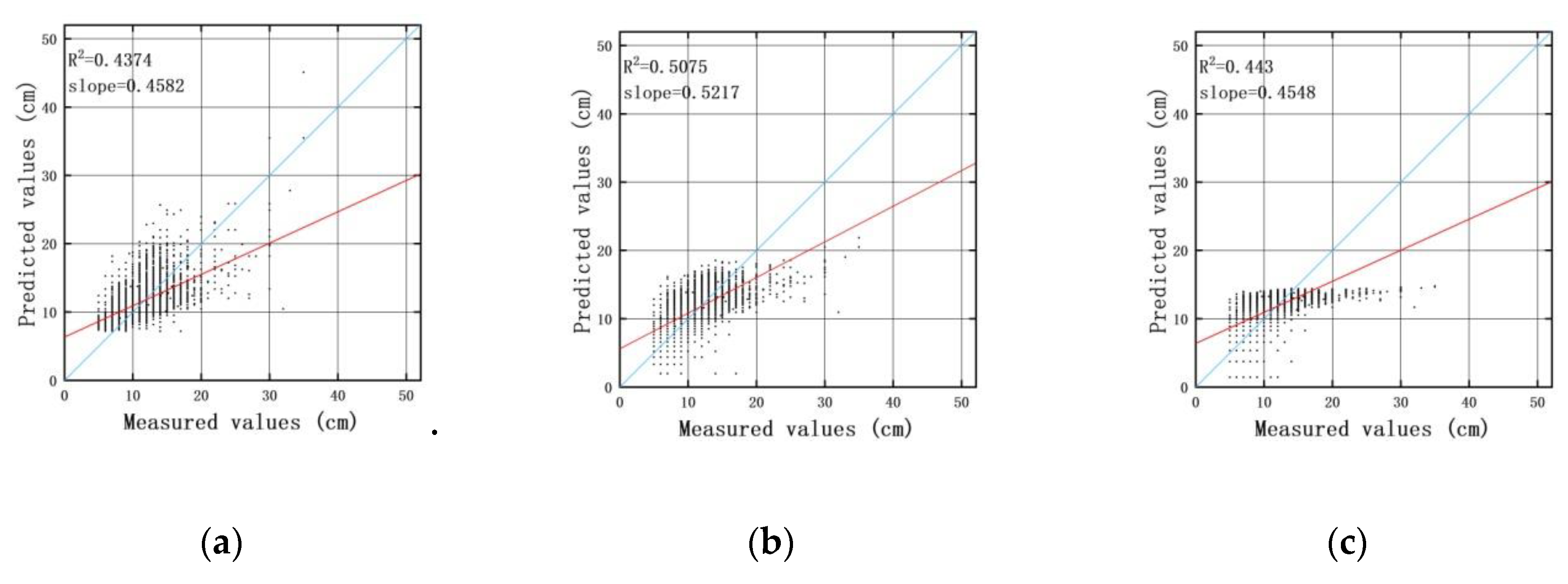
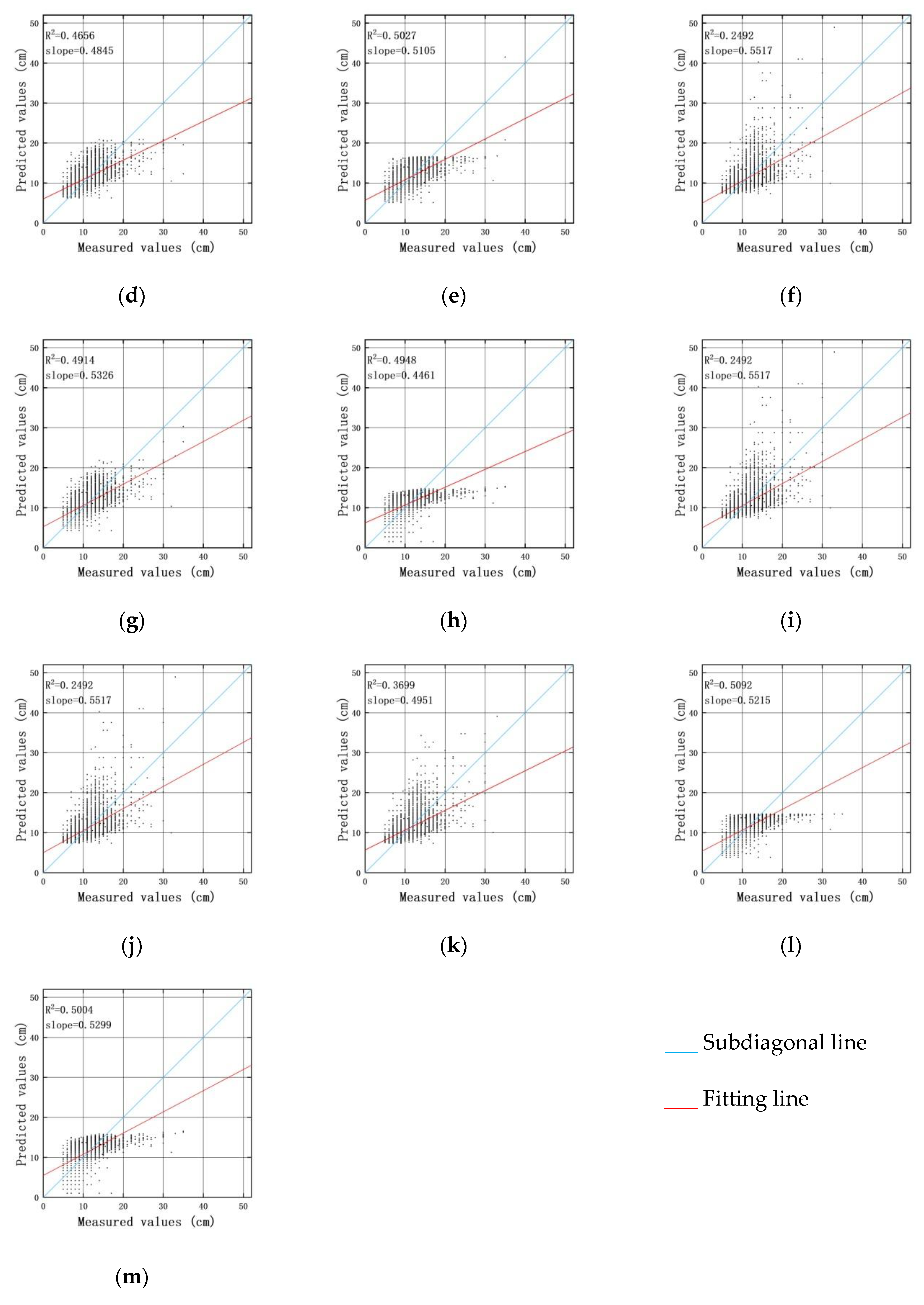
Based on the research data that were divided into 25,000 training samples and 10,763 testing samples (Table 1), the 13 empirical age–DBH models (Table 2), in which the only independent variable was the tree age, were used to fit the relationship between the tree age and DBH of the forest subcompartments (Table 3) and to predict the DBH (Table 4). The modeling results of the 13 empirical models had R² values between 0.438 and 0.592. The MAPEs ranged from 15.63 to 19.3%, which means that the accuracies of the predictions were above 80%. The amplitude of R² prediction results obviously increased with a range of 0.2492–0.5092 compared to the modeling results. However, the Gompertz model provided the strongest generalizability with the best performance metrics of 1.7622 cm in MAE, 15.63% in MAPE, and 0.5092 in R², which were even better than the modeling result. These findings are similar to those reported by Xu et al. and Lin et al. [57,58]. With the various size classes of DBH, Xu et al., taking 90 felled maple trees (Liquidambar formosana Hance) as the study object, and Lin et al., taking 90 felled Schima superba trees (Schima superba Gardn. et Champ.) as the study object, found that Gompertz was the optimal model, whether for DBH, tree height, or volume [57,58].

After the correlation analysis, the four factors from the inventory data for forest management planning and design and DEM were retained for further modeling and prediction by MLR and GRNN, namely, the elevation, age of the tree, canopy density, and the number of trees per hectare, as these satisfied p ≤ 0.01 and r ≥ 0.1. The order of absolute values of the correlation coefficients from high to low was the age of the tree, canopy density, the number of trees per hectare, and elevation. The R for the relationship between the number of trees per hectare and the DBH was negative, which indicated that competition among the trees affected the growth in DBH. This finding is similar to those reported by Luo et al. [53], with a negative correlation between the number of trees per hectare and DBH, and similar to Escalante et al. [54], in which forest stand simulations under fixed conditions indicated that the probabilities of diameter growth increase with site productivity increase, and decrease with an increase in the stand density index.

From the remote sensing images, the seven factors of bands 2–7 and DVI were also retained. The order of the absolute values of the correlation coefficients from high to low was B3, B2, B5, DVI, B6, B4, and B7.

The prediction results obtained by MLR and GRNN (Table 7) when using more environmental factors, such as topography and soil, were much better than those produced by the 13 empirical age–DBH models. This indicates that the environmental factors are beneficial for the estimation of DBH.

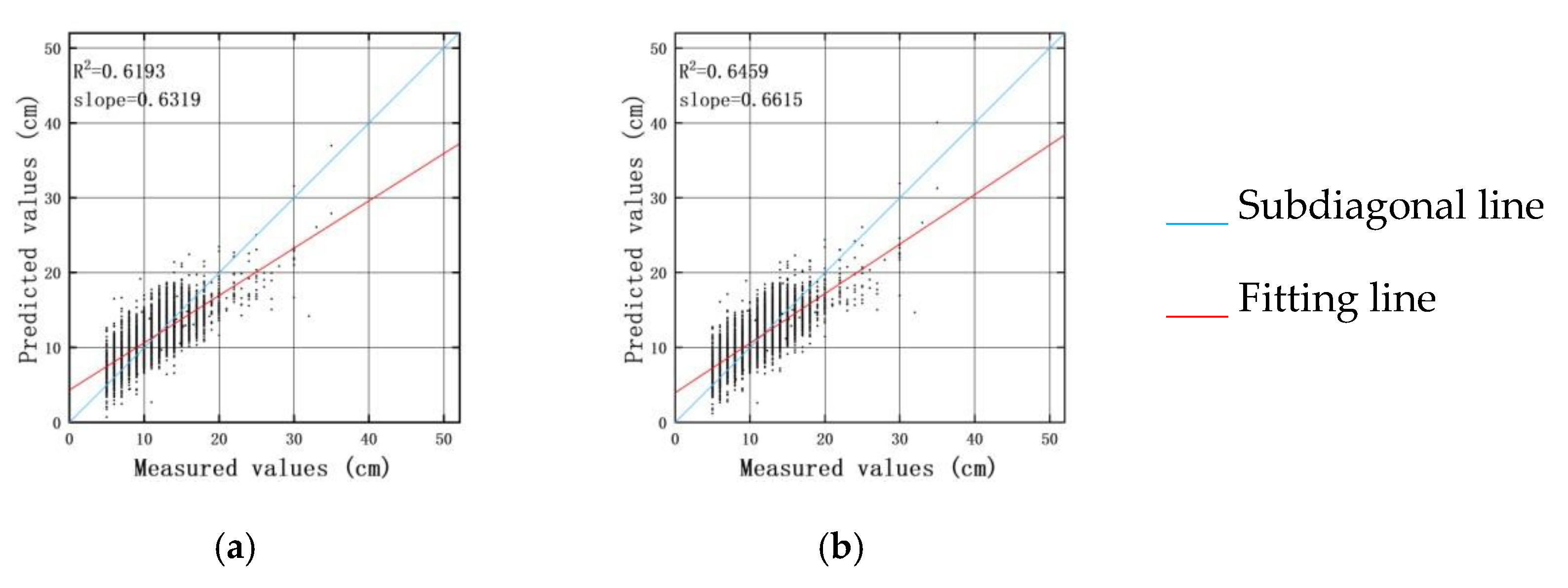
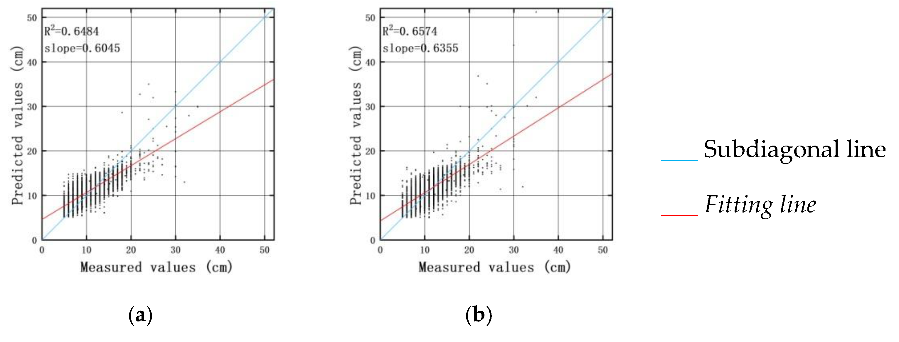
By adding the remote sensing image factors, the experimental results from MLR were further improved from 1.6006 cm in MAE, 14.96% in MAPE, 2.0707 cm in RMSE, 0.6193 in R², and 0.0854 in TIC to 1.5300 cm in MAE, 14.38% in MAPE, 1.9976 cm in RMSE, 0.6459 in R², and 0.0823 in TIC. Correspondingly, the experimental results from GRNN were improved from 1.4926 cm in MAE, 13.99% in MAPE, 1.9980 cm in RMSE, 0.6484 in R², and 0.0826 in TIC to 1.4688 cm in MAE, 13.78% in MAPE, 1.9655 cm in RMSE, 0.6574 in R², and 0.0810 in TIC. This indicates that the remote sensing image factors are beneficial to the estimation of DBH.

Regardless of whether remote sensing image factors were included, the experimental results from GRNN—with lower MAE, MAPE, RMSE, and higher R²—were better than those of MLR. In the forestry application of artificial neural networks (ANNs), He et al. used the ANN method to simulate and predict the DBH for different age groups and showed that the mean predictive accuracy of DBH for bamboo stands was satisfactory [16]. Vieira et al. estimated the growth of DBH and height of eucalyptus trees in 398 plots using artificial intelligence techniques (AIT), including ANN and an adaptive neuro-fuzzy inference system, and obtained good accuracy [59]. Although different from previous studies, this study still achieved an acceptable accuracy to predict DBH at the subcompartment’s level with GRNN based on more diversified tree species and a wider range of samples totaling 35,763. Thus, the prediction results are more convincing.

6. Conclusions

The prediction results by MLR and GRNN when using more environmental factors, such as topography and soil, were much better than those produced using traditional empirical age–DBH models. The use of comprehensive factors, including ecological and biological factors, was beneficial for improving the prediction accuracy of both the MLR and GRNN models. When remote sensing factors were included, the performance metrics were further improved in the MLR and GRNN models, with MAE decreasing by 0.0238 and 0.0706 cm, MAPE decreasing by 0.21% and 0.58%, RMSE decreasing by 0.0325 and 0.0731 cm, R² increasing by 0.09 and 0.0266, TIC decreasing by 0.0031 and 0.0016, respectively. Regardless of whether remote sensing image factors were included, the experimental results produced using GRNN were better than those using MLR. For modeling and prediction based on more complex tree species and a wider range of samples, the GRNN model is more desirable due to its stronger generalizability.