Article

Estimating Crown Structure Parameters of Moso Bamboo: Leaf Area and Leaf Angle Distribution

1
State Key Laboratory of Subtropical Silviculture, Zhejiang A & F University, Hangzhou 311300, China
2
Key Laboratory of Carbon Cycling in Forest Ecosystems and Carbon Sequestration of Zhejiang Province, Zhejiang A & F University, Hangzhou 311300, China
3
School of Environmental and Resources Science, Zhejiang A & F University, Hangzhou 311300, China
*
Author to whom correspondence should be addressed.
Forests 2019, 10(8), 686; https://doi.org/10.3390/f10080686
Submission received: 4 July 2019 / Revised: 10 August 2019 / Accepted: 12 August 2019 / Published: 14 August 2019
(This article belongs to the Special Issue Modeling of Forest Structure and Dynamics)

Abstract

:
Both leaf area (LA) and leaf angle distribution are the most important eco-physiological measures of tree crowns. However, there are limited published investigations on the two parameters of Moso bamboo (Phyllostachys edulis (Carrière) J. Houz., abbreviated as MB). The aim of this study was to develop allometric equations for predicting crown LA of MB by taking the diameter at breast height (DBH) and tree height (H) as predictors and to investigate the leaf angle distribution of a MB crown based on direct leaf angle measurements. Data were destructively sampled from 29 MB crowns including DBH, H, biomass and the area of sampled leaves, biomass of total crown leaves, and leaf angles. The results indicate that (1) the specific leaf area (SLA) of a MB crown decreases from the bottom to the top; (2) the vertical LA distribution of MB crowns follow a “Muffin top” shape; (3) the LA of MB crowns show large variations, from 7.42 to 74.38 m2; (4) both DBH and H are good predictors in allometry-based LA estimations for a MB crown; (5) linear, exponential, and logarithmic regressions show similar capabilities for the LA estimations; (6) leaf angle distributions from the top to the bottom of a MB crown can be considered as invariant; and (7) the leaf angle distribution of a MB crown is close to the planophile case. The results provide an important tool to estimate the LA of MB on the standing scale based on DBH or H measurements, provide useful prior knowledge for extracting leaf area indexes of MB canopies from remote sensing-based observations, and, therefore, will potentially serve as a crucial reference for calculating carbon balances and other ecological studies of MB forests.

1. Introduction

As “the major non-wood forest product and wood substitute”, bamboo is widely distributed in tropical, subtropical, and warm, temperate regions between 46°N and 47°S, which covers a total area of 31.47 million hectares, accounting for 0.78% of the global forest area [1]. In Asian countries, bamboo forests have been expanding rapidly for the past 50 years [2]. China possesses the largest bamboo forest with an area of more than 6.01 million hectares, which accounts for approximately 2.97% of the total forested area nationally [3]. The area of Moso bamboo (Phyllostachys edulis (Carrière) J. Houz., abbreviated as MB) has reached 4.43 million hectares, which is 73.71% of the bamboo forested area in China [3]. Many efforts have been made to quantify ecological properties of MB, such as stand-scale transpiration [4], canopy chlorophyll content [5], and soil respiration of MB forests [6]. Characterized by fast growth and strong carbon sequestration abilities, MB forests show great potential to be a substantial carbon sink and, thus, play a significant role in addressing global climate change [4,7,8,9,10,11]. Carbon exchange between the atmosphere and MB crowns is significantly quantified and explained by leaf area (LA) and leaf angle distribution, which are the two most important crown structure parameters [12,13].
Leaf area index (LAI), i.e., projected leaf area per unit surface area of the ground, is generally used to quantify LA in forestry, eco-physiology, and remote sensing communities [14,15]. Recently, much attention has been paid to estimate the LAI of MB canopies based on satellite remote sensing techniques. Xu et al. [5,16] developed empirical and correction models, respectively, to estimate LAI for MB canopies using the Moderate Resolution Imaging Spectroradiometer (MODIS) data. Li et al. [17] and Mao et al. [18] developed assimilation methods to improve the MODIS LAI time series of MB forests. Furthermore, Li et al. [19] estimated aboveground biomasses of MB forests using the MODIS LAI spatiotemporal data and machine learning algorithms. Additionally, Mao et al. [20] analyzed the spatiotemporal pattern and heterogeneity of carbon fluxes of the bamboo forest in Zhejiang Province of China, based on the assimilated LAI. To validate LAIs retrieved from satellite remote sensing images, LAIs indirectly estimated using ground-based digital hemispherical photography (DHP) are taken as surrogate truths [17,18,21] because its field work requirements are more efficient, less expensive, and more user friendly and eco-friendly [22]. However, the DHP-based LAI is always underestimated [23,24,25] because of photographic over exposure [26,27], scattered radiation influences [28], non-random distributed leaves [29,30,31], and high leaf density influences [32]. Direct LA measurements, such as destructive harvesting, litter collection, and allometric equations, are widely accepted as reliable methods and, consequently, important validations for indirect methods such as the DHP method [31,33]. On this issue, allometric methods are more suitable for a large number of forest types because of the relatively stable physical or physiological interrelations among stem dimensions, crown dimensions, LA, and biomass amounts [14,31,34]. Previous studies reported many allometric relationships with accessible tree traits as independent variables to estimate LAs of several specific tree species. These allometries generally relate LA to tree characteristics such as diameter at breast height (DBH) and tree height (H) [13,35,36,37]. However, there are no validation studies to prove the reliability of the estimated LA of MB by indirect methods. Therefore, development of allometric models for estimating the LA of MB is essential to validate LAs retrieved by indirect methods and to facilitate other ecological studies on MB.
On the other hand, leaf angle distribution, i.e., the probability density of the leaf angle [38], is also one of the most commonly used structural characteristics of a vegetation canopy. Leaf angle distribution influences the spectral reflectance and radiation transmission properties of vegetation canopies and, hence, interception, absorption, and photosynthesis [39,40,41]. A few leaf angle distribution estimations have been reported for different tree species [42,43,44]. However, little is known about the leaf angle distribution of MB crowns. In general, three types of methods were used for in situ leaf inclination angle measurements, and subsequently for leaf angle distribution modeling, including direct measurements by mechanical inclinometers [45], the indirect photographic method [43,44,46], and indirect three-dimensional digitizing of individual plant elements using specialized instrumentation [42]. The direct mechanical inclinometer measurement has been a traditional and reliable method; however, it is laborious and requires careful measurements of many leaf surfaces [40]. For example, Pisek et al. [44] evaluated canopy non-randomness based on clinometer measurements of 100 leaf angles of three birch trees. For simplification of leaf angle measurements, Ryu et al. [43] developed a photographic method that analyzing leveled digital camera images of canopies consisting of flat leaves. This method allows for a rapid and non-contact estimation of leaf angles and has been applied to several broadleaf canopies. They measured 1200 leaf angles of oak crowns to estimate leaf projection functions, and then the estimated erectophile distribution was used to retrieve LAIs based on a modification of Lambert-Beer’s law. Piayda et al. [47] also determined the leaf angle distribution of a sparse, savannah-type cork oak canopy based on 1561 leaf angle measurements using the photographic method to compare three non-destructive LAI measurement techniques. Another way to obtain leaf angle measurements is to improve inclinometer measurements based on the indirect three-dimensional digitizing method. For example, a leaf angle estimation method based on retrieved Terrestrial LiDAR Scanning (TLS) data was recently developed by Vicari et al. [41]. However, Zou et al. [40] pointed out that with indirect methods, it is almost impossible to differentiate the effects of leaf angles on canopy transmittance from other structural influences.
The objectives of this investigation are (1) to develop allometric equations for LA estimations of a MB crown based on DBH or H and (2) to find the leaf angle distribution of MB crowns.

2. Materials and Methods

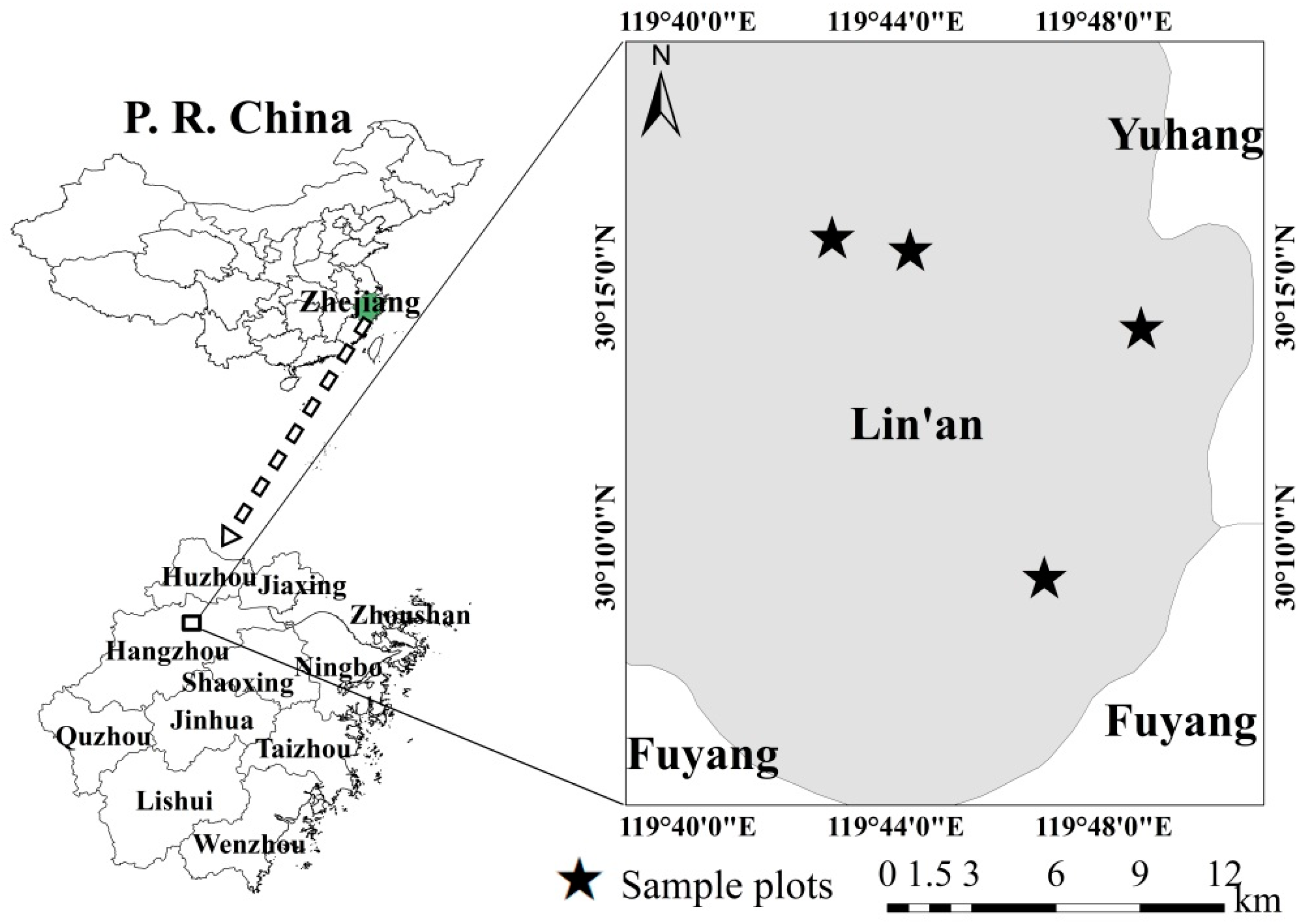
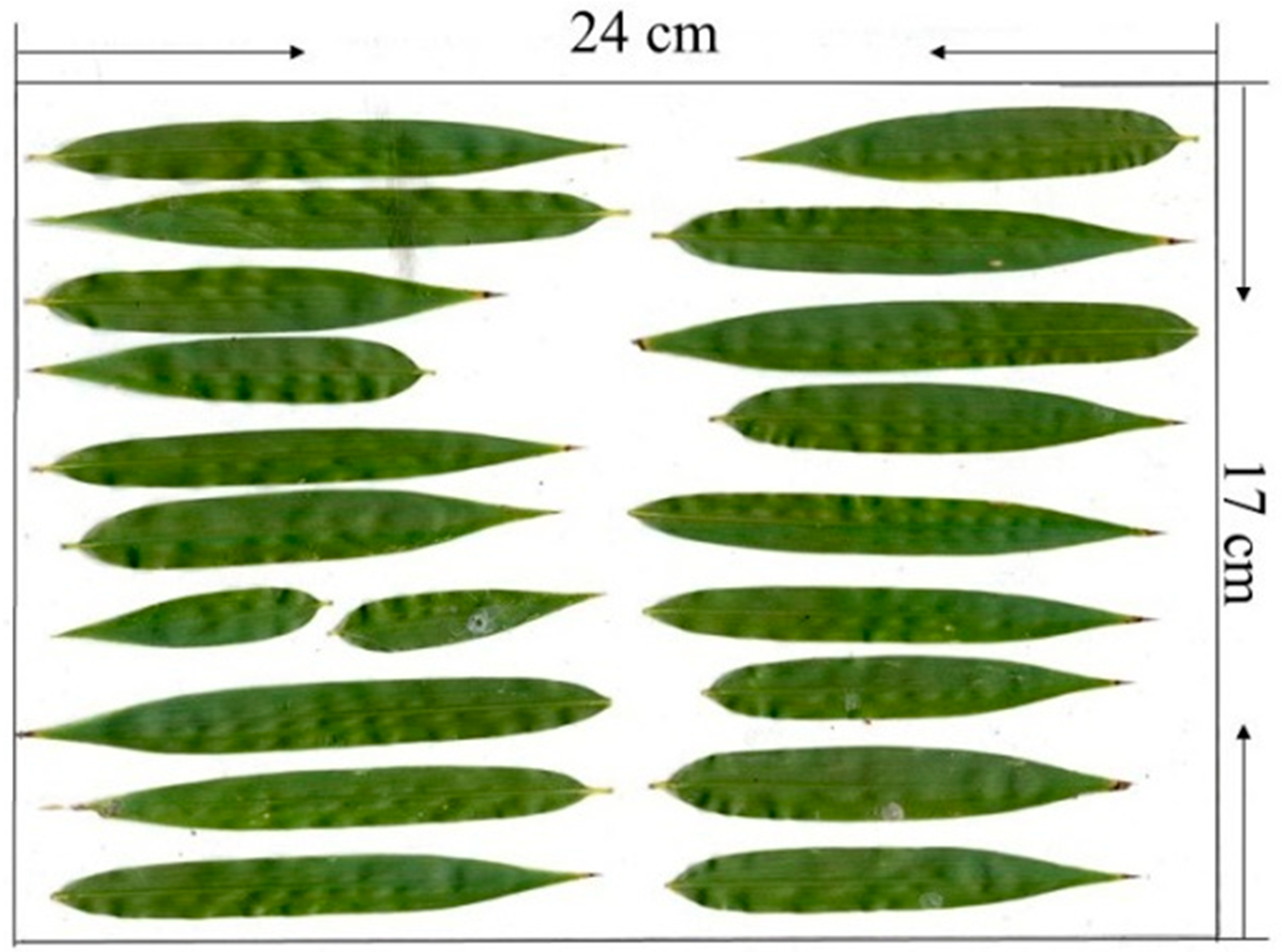
2.1. Study Area, Destructive Sampling, and Laboratory Procedures

The study area was in Lin’an city (118°51′–119°52′ E, 29°56′–30°23′ N), southeast of China. Lin’an has an undulating terrain in the east and mountainous regions in the west, with elevation ranging from 10 to 1580 m. Lin’an is in the subtropical monsoon climate zone with a mean temperature of 15.9–17.0 °C and an average annual precipitation of 1614 mm. MB forests are the dominant species in this area. Other vegetation types include coniferous evergreens, broad-leaved evergreens, and mixed coniferous and broad-leaved forests. The primary soil types are red and yellow soils (by Chinese soil taxonomy). A total of 29 healthy and well-formed MB crowns (i.e., there were no signs of defoliation and pest and disease damage) were destructively sampled in late August and early September 2018. We randomly sampled 2, 4, 11, and 12 crowns within four pure MB plots, respectively (Figure 1). The sampled bamboo crowns were away from residential areas, roads, and reservoirs. In addition, the spatial distance between each of the sampled MB crowns was larger than 20 m.
Several plant characteristics of the 29 MB crowns were measured and recorded for LA estimation, including DBH, H, total leaf biomass of each crown, and the biomass and area of the sampled leaves in each of the 29 crowns (Table 1). DBHs of the 29 MB crowns were measured using a diameter tape, and H was measured from its trunk base to the top of a crown, using a measuring tape, after cutting down its trunk. Each of the 29 crowns was divided equally into three sections (top, middle, and bottom). About 120 leaves in each section were randomly selected as samples. The sampled leaves were rapidly scanned using an Epson perfection V30 SE scanner (Seiko Epson Corporation, Nagano, Japan) to measure LA to avoid leaf deformation caused by water loss. A white sheet of paper (17 cm × 24 cm) was placed under the sampled leaves during the scanning process as a spatial reference for LA measurements. However, the sampled leaves of some sections were less than 120 pieces because low-quality scanned images were abandoned, such as the contaminated reference paper, and the folded or overlapped leaves. Figure 2 shows an example of the scanned images. The scanned images were classified as leaves and background using MATLAB 2014a software based on digital image processing techniques. Then, the LA of each image was calculated based on the ratio of the leaf pixels and total pixels within the 17 cm × 24 cm rectangle. All sampled leaves of the three sections in each of the 29 MB crowns were separately packed in paper bags and oven-dried at 80 °C for 48 h until their dry weight was constant. Then, the dry mass of sampled leaves was measured using an electronic balance (Wuxin Weighing Apparatus Co., Ltd, Zhejiang, China) with an accuracy of 0.0001 g. The total leaf biomass for each of the 29 crowns was measured in the same way as the sampled leaves.
Leaf angle measurements were conducted to estimate the leaf angular distribution. The leaf inclination angle α is defined as the angle between the leaf surface (normal) and the zenith from 0° to 90°. We carefully measured and recorded 312 leaf inclination angles (104 × 3 sections = 312 leaves of a crown) randomly from each of the 29 crowns using a digital obliquity sensor (DXL360S, Jingyan, Inc., Guangdong, China).

2.2. Allometric Equations for LA Estimation

The following three steps were carried out to develop the allometric relationships between the LA of a crown and DBH or H: (1) the specific leaf area (SLA) was calculated based on the sampled LA (Ssampled) and biomass (Bsampled) for each section of the 29 MB crowns [48,49]:
S L A = S s a m p l e d / B s a m p l e d ,
(2) LA of a crown (Scrown) was estimated depending on the total leaf biomass of a crown (Bcrown) and SLA [36]:
S c r o w n = S L A · B c r o w n ,
and (3) DBH and H were not used as simultaneous predictors because of the strong linear correlation between DBH and H (R2 = 0.88, p < 0.0001). Linear, exponential, and logarithmic regressions were used for Scrown estimations:
Y = a · X + b ,
Y = a · X b ,
Y = a · e b · X ,
where X is DBH or H, Y is LA of a crown, and a and b are the equation parameters. Because the assumption of the heteroscedasticity was violated for nonlinear regression measurements in our original scale, Equations (4) and (5) were log-transformed [50,51,52]:
ln Y = a · ln X + b ,
ln Y = a · X + b ,
where a′ and b′ are the log-transformed equation parameters. a′ equals b and b′ equals ln a. The transformation, however, introduced a systematic bias, which can generally be corrected with the following correction factor [52,53,54,55]:
C F = e S E E 2 / 2 ,
where CF is the correction factor, and SEE is the standard error of the estimate, calculated as follows:
S E E = i = 1 n ( ln Y i ln Y ^ i ) 2 / ( n 2 ) ,
where Y i and Y ^ i are observed and predicted biomass values of the ith sample, respectively, and n is the number of samples. Equations (6) and (7) were back-transformed to get LA equations [52]:
Y = C F · e b · X a ,
Y = C F · e b · e a · X ,
The goodness-of-fit of the models were evaluated by the coefficients of determination (R2) and root-mean-square error (RMSE). In addition, leave-one-out cross validation (LOO) was used for model validation [56,57].

2.3. Leaf Angle Distribution and Leaf Projection Function

The leaf projection function G(θ) is the projection coefficient of a unit area of foliage on a plane perpendicular to the view/solar zenith angle θ. G(θ) is generally used for classifying leaf angle distribution f(α) in the remote sensing community [43,44]. The value of the G-function can be calculated by integrating f(α) over α:
G ( θ ) = 0 π / 2 A ( θ , α ) f ( α ) d α ,
where A is the projection coefficient for α and θ according to the theory by Wilson [58]:
A ( θ , α ) = { cos ( α ) · cos ( θ ) α + θ 90 ° cos ( α ) · cos ( θ ) · [ 1 + 2 / π · ( tan ( γ ) γ ) ] α + θ > 90 ° ,
where γ = arccos ( cot ( α ) · cot ( θ ) ) .

3. Results

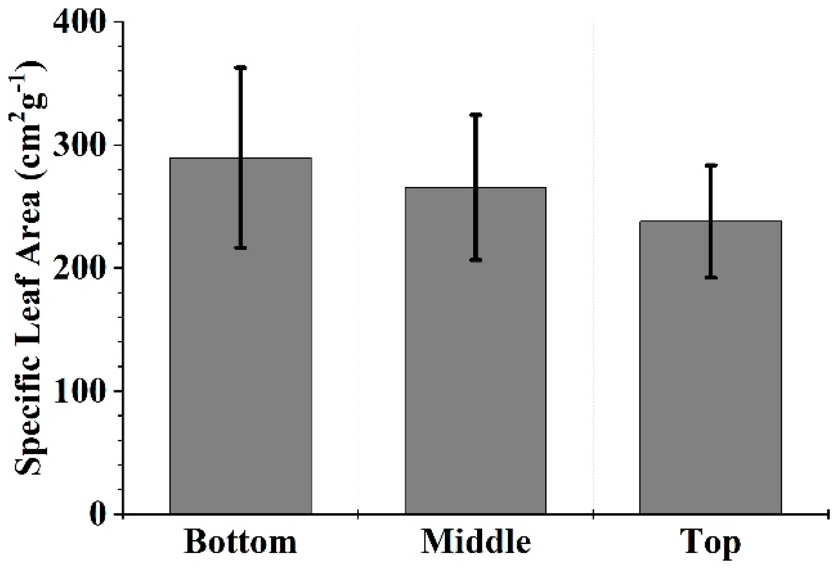
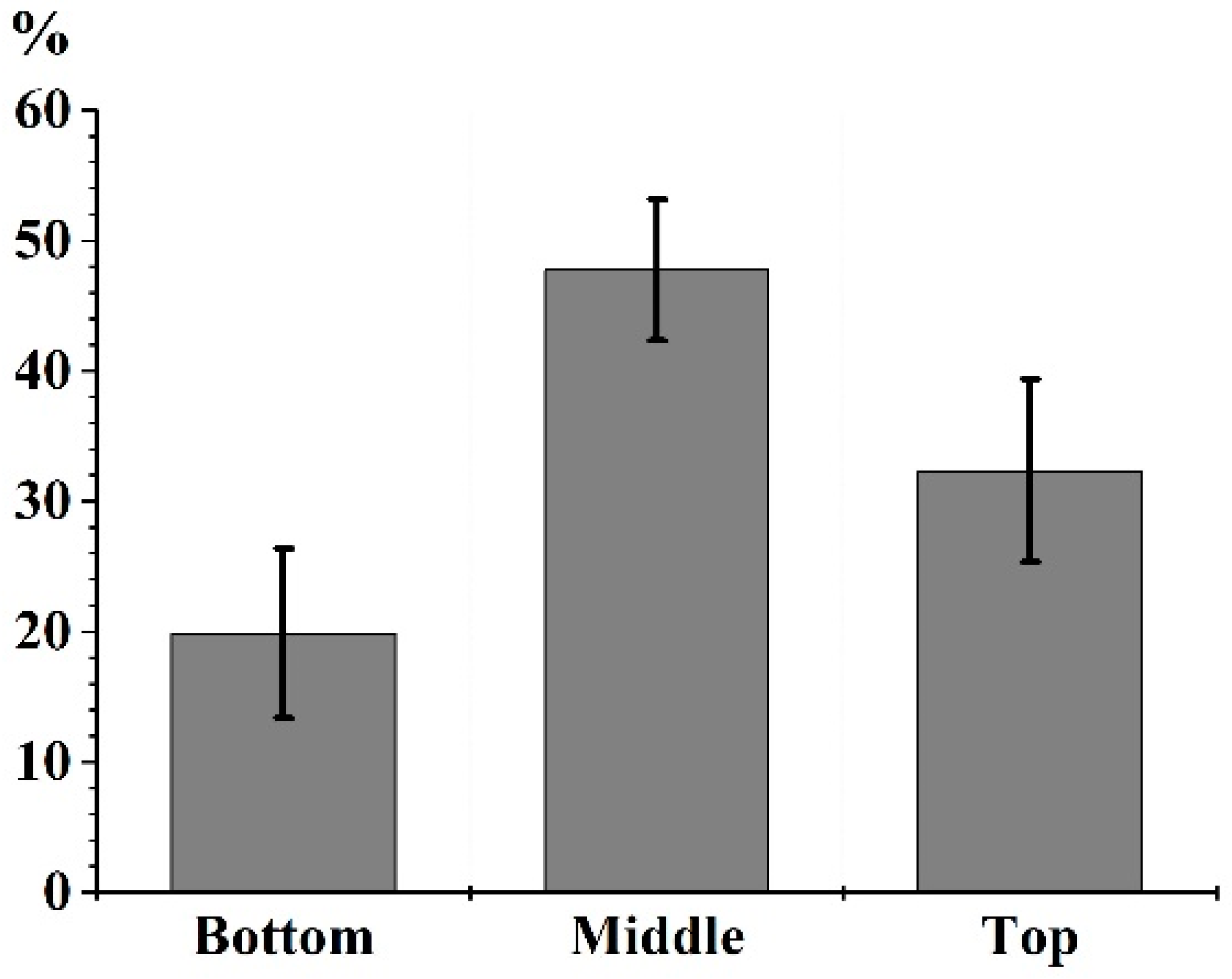
3.1. LA of a MB Crown

As for the 29 sampled MB crowns, mean SLA values of the top, middle, and bottom sections were 237.76 cm2·g−1 (from 158.62 to 333.52 cm2·g−1), 265.35 cm2·g−1 (from 173.58 to 381.55 cm2·g−1), and 289.54 cm2·g−1 (from 152.21 to 466.37 cm2·g−1), respectively (Figure 3). The SLA values tended to decrease from the bottom to the top of the crown. The negative relationship coincided with the findings of other tree species reported in previous studies [48,59,60]. However, the reason for that phenomenon is still unclear [59]. Potential explanations will be given in the discussion section.
Considering SLA varies with height in a MB crown, the LA of a crown should be the sum of LA estimated from the top, middle, and bottom sections, respectively. The estimated LA, which varied from 7.42 to 74.38 m2, showed more than 10 fold divergence among the 29 MB crowns because of the large differences in leaf biomass (Table 1). On the other hand, the average vertical LA distribution of the 29 crowns showed a significant “Muffin top” character (Figure 4). Nearly half of LA grew in the middle section of a crown, about 30% of the LA was in the top section, and the remaining 20% LA was situated in the bottom section of the crown. This type of LA distribution has generally been reported with broad-leaved crowns [15].

3.2. Allometric Equations for LA Estimation

Both DBH and H are popular structural parameters used to estimate the crown-scale LAs based on allometric equations [14,34,36,61]. In this study, empirical equations with one unknown independent variable, rather than with two unknown independent variables (DBH and H), were used to develop allometric relationships in order to avoid multicollinearity problems, as there was a strong, linear relationship between DBH and H (R2 = 0.88, p < 0.0001). Therefore, six allometric relationships were developed for LA estimations based on three types of regression models, including linear, exponential, and logarithmic regressions, and two predictors, including DBH and H, respectively. Table 2 shows the regression parameters and the goodness-of-fit statistics of the six allometric relationships. R2 values of the six models showed minor differences, from 0.7789 to 0.8211. This indicates no single relationship was significantly outstanding among the six allometric relationships. RMSE estimated based on linear regression cannot be compared to the other nonlinear regressions because Equations (3)–(6) were log-transformed. As for the linear LA models, RMSE did not show a significant divergence between using H and DBH, because of the high correlation of the two predictors. The RMSE values of the nonlinear allometric relationships also had no big differences. The highly reliable relationships among H, DBH, and LA of MB crowns can be explained by the species-specific branching pattern that depends on genetic and environmental influences [62].
The six allometric relationships in Table 2 were validated based on the leave-one-out cross validation (Figure 5). LOO validations confirm the similar and highly reliable relationships between predicted and observed LA data for the six models. The results indicate that any one of the three types of regression methods can be used for the estimation. Both DBH and H are also suitable for the LA estimations of a MB crown.

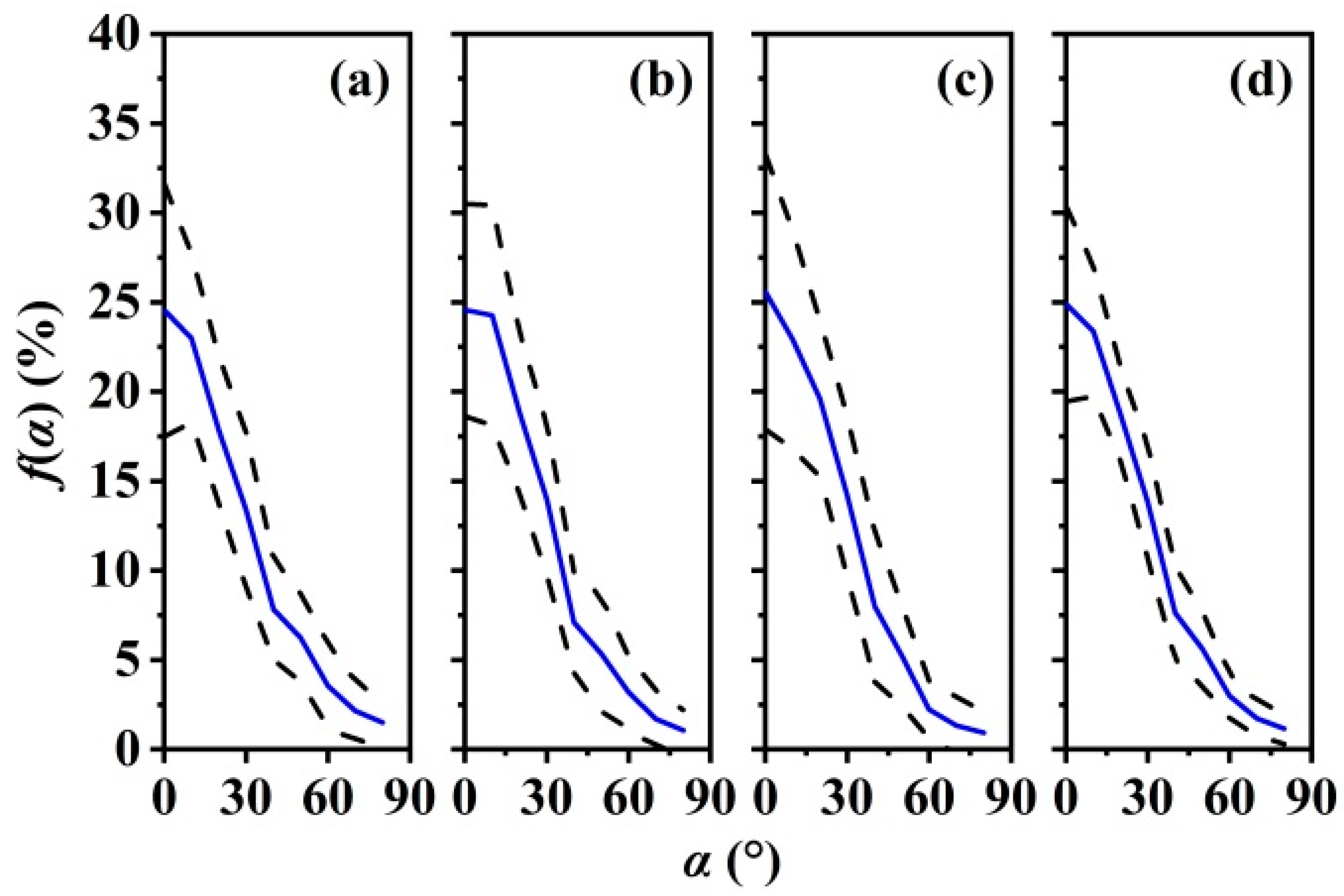
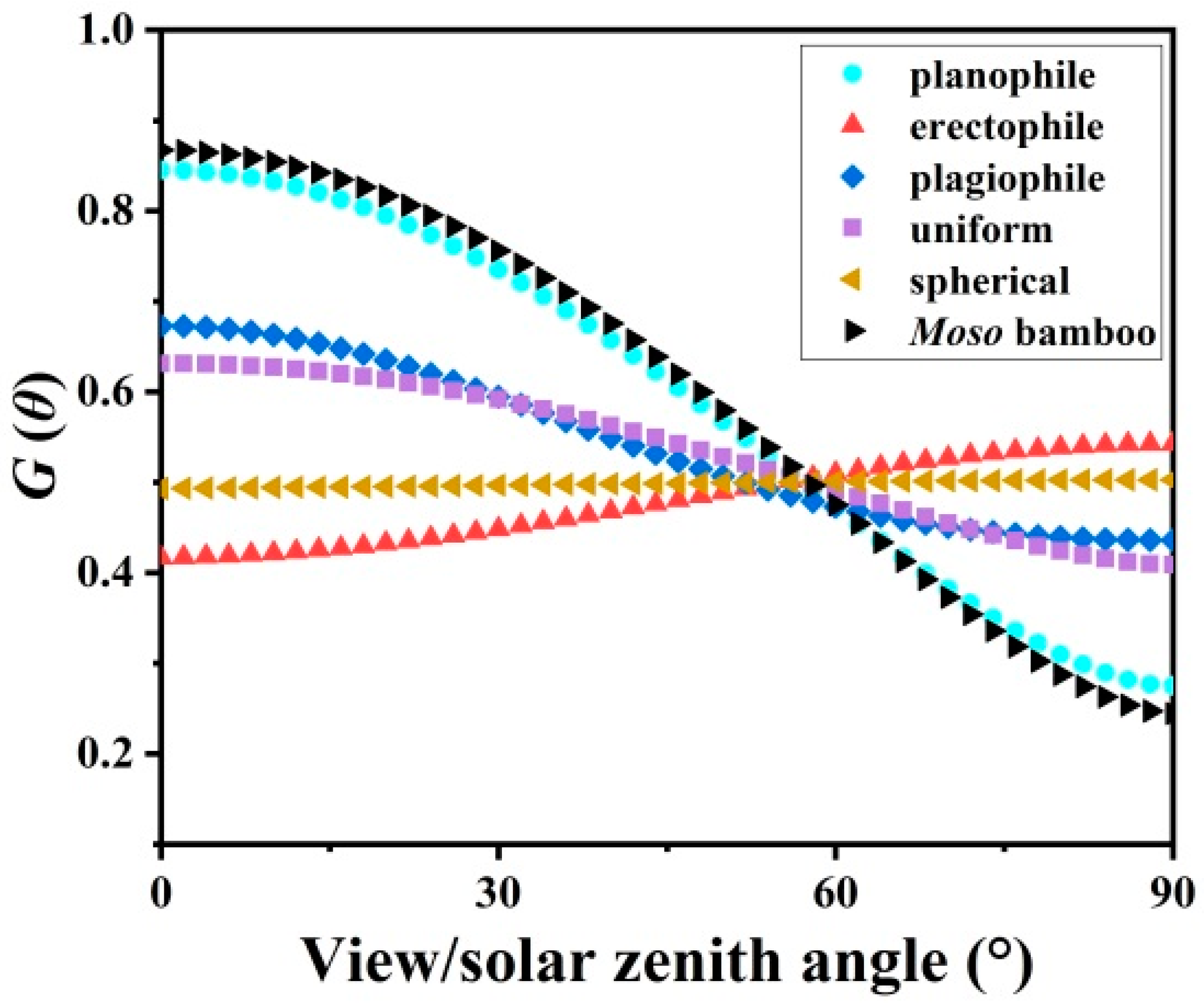
3.3. Leaf Angle Distribution f(α) and Leaf Projection Function G(θ)

Figure 6 is the leaf angle distribution f(α) of MB crowns with a 10° leaf angle interval. It can be found that: (1) The average leaf angle proportion decreased significantly with increasing α; and (2) the differences of f(α) among the top, middle, and bottom sections were not significant. Therefore, it is not necessary to specify sampling positions in the MB crown for leaf angle measurements. The estimated f(α) using total leaf angle data of a MB crown is shown in Figure 6d.
G(θ) of MB crowns was simulated based on f(α) according to Equation (12) (Figure 7). Compared to the five typical leaf angle distributions, including the erectophile, planophile, plagiophile, spherical, and uniform cases [63], G(θ) of MB crowns tends to be planophile.

4. Discussion

4.1. Specific Leaf Area

SLA is an important conversion factor for estimating LA [37,60]. This study found that SLA values increased from top to bottom of a MB crown (Figure 3). This relationship is consistent with most previous studies with varied tree species [48,59,60] and is generally explained by the following two main possible reasons, which refer to different leaf strategies in response to environmental pressure and constrains [64]. One reason concerns the fall in water potential [59]. With a tree stem growing taller, the stem conductance reduces [61,65]. A further reduction in water potential may induce a reduction in turgor pressure. Then, stomata would potentially close, and cell expansion would likewise be reduced. Furthermore, such water stress might be associated with the development of xeromorphic features, including thick cuticles and lignified cell walls, both of which would tend to reduce SLA. Another reason is related to the expression of the plant species’ ability to cope with changing light [66,67,68,69,70]. Light conditions for leaves in the lower crown are shadier and worse compared to that of the leaves in the upper crown; therefore, a larger SLA is likely an adaptation to more efficiently intercept light in low-light conditions [60,71,72]. Certainly, both the hydraulic limitations of greater branch height and light availability may combine to impact SLA [70]. Although these two explanations have been accepted by previous studies to a certain extent, detailed physiology studies for the MB species are worth exploring further to uncover more potential reasons.
Previous studies found that the higher SLA in broad-leaved trees, relative to evergreen conifers, fit the trend of a decreasing SLA with increased leaf lifespan [73,74,75,76]. As expected, the SLA value of MB, ranging from 152 cm2·g−1 to 466 cm2·g−1, is a typical example of broadleaf trees when compared with several published SLA cases (Table 3 and Table 4). Because of the unique biological rhythm of MB’s leaf growth, new bamboo usually grows leaves in June of its first year; these initial leaves fall in the next spring, and new leaves quickly emerge. The new leaves have a life span of 2 years, thus, replacement occurs biennially [77,78,79]. Therefore, the short lifespan of MB leaves results in a high SLA value.

4.2. LA Estimation of MB

To quantify total LA in the field, this study indicates that DBH is a reliable and easy scalar to measure, and validation proves that the empirical relationships between the LA of MB and its DBH are highly significant. On the contrary, in many cases of forest inventories, H of MB is obtained through eye estimations by skilled workers under complicated forest conditions, including tree tops that are hidden by the canopy layer, bending growth of crowns, and a sloping background. This can be a source of error that needs to be considered. On the other hand, the strong, linear relationship between the DBH and H of MB agrees with the results by previous studies for other tree species, which indicate that DBH is also used as a reliable crown trait for H estimations [11,55,88,89], and using both DBH and H as independent variables to estimate LA cannot significantly improve, or even reduce, the accuracy of estimations [13,90,91]. Therefore, DBH is a better predictive variable for the allometry of LA of MB crowns.
The linear, allometric equations showed as good of a performances as those of the nonlinear equations, including the exponential and logarithmic regressions. This means that the nonlinear models do not explain more of the variation and do not fit the data better than the linear models. Therefore, a linear, allometric relationship is preferred for estimating the LA of MB because it is easy to use. In addition, it should be kept in mind that, when using the developed allometric equations of this study, regression should not be applied beyond the range of observations used to develop the model.
Does the LA of a MB crown change with the invariant DBH and H? And does the developed allometry of LA lose efficacy if LA changes within a MB crown? The “pipe model” theory [92] potentially explains this problem. It indicates that a given LA is supplied with water from a respective quantity of conducting pipes. Different from other tree species, MB, which belongs to the Poaceae family, usually can reach its maximum DBH and H in only 40–60 days. Once it enters the second growth stage (strength increase and biomass accumulation), DBH and H will not increase anymore because of the lack of cambium [8]; hence, no new conducting pipes are produced as the tree ages. On the other hand, as on the tree ages, a part of the conducting pipes might be clogged. Therefore, the potential decrease in water supply theoretically leads to the reduction of the LA of a MB crown according to the “pipe model” theory. However, this reduction was not found in the 29 sampled crowns at various ages, from 1 to 5 years. That was because a MB crown is harvested usually at 6–8 years, and variations of its conducting pipes do not significantly influence the quantity of LA in such a short lifespan. In addition, the LAs of this study were not sampled at the leaf replacement stage (field work was conducted during late August and early September). Therefore, all developed allometric relationships are applicable, except during the leaf replacement stage of MB.

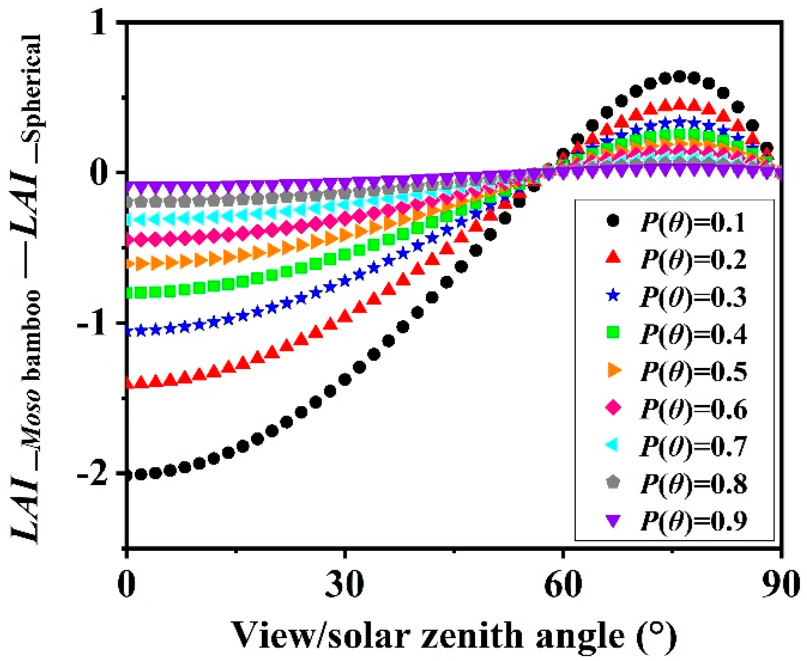
4.3. Leaf Angle Influence on LAI Estimation

A simple LAI inversion case, using an inappropriate G(θ), was taken as an example to show the influence of leaf angle distribution on ecological studies of MB. In the remote sensing community, G(θ) is one of the critical canopy structure parameters used for LAI estimation and is based on the modified Lambert–Beer’s law:
P ( θ ) = e G ( θ ) · L A I · Ω ( θ ) / cos ( θ ) ,
where P(θ) is the gap fraction of a canopy, which is generally obtained by hemispherical optical instruments such as in DHP [93,94]; and Ω(θ) is the clumping index, which is used for quantifying leaf spatial distribution within a canopy. Here, Ω(θ) is assumed as 1 to represent a random spatial distribution of leaves. Generally, a spherical leaf angle distribution (G(θ) ≈ 0.5) is considered as the surrogate truth of G(θ) in Equation (14) when f(α) is unavailable [95,96]. However, this study found that the G(θ) of MB was far from the spherical case and was close to the planophile case. Based on Equation (14), the error for the LAI estimation of MB using the spherical case can be estimated (Figure 8). The results show that the LAI of a MB canopy is overestimated with view/solar zenith angles from 0 to 57.5°, and the overestimation reaches up to 2. However, LAI is underestimated with view/solar zenith angles from 57.5° to 90°, and the maximum underestimation is 0.62 at a 77° view/solar zenith angle. With a decreasing gap fraction at the same view/solar zenith angle, the error of the LAI estimation increases. However, the error of the estimation is at a minimum and close to 0 at 57.5° for all gap fractions. This is also the reason why many previous LAI estimations used a 57.5° view/solar zenith angle when f(α) is unavailable [97,98,99]. Considering the significant error using inappropriate leaf angle distributions, we suggest using the modeled G(θ) in this study to estimate LAI of MB, especially for the cases with large gap fractions.

5. Conclusions

This study represents the first attempt to report species-specific allometric equations for the crown-scale LA estimations of MB and its leaf angle distribution. The simplest and most efficient linear regression uses the predictor DBH, which is easy to measure in the field, and is recommended for LA estimations of MB. On the other hand, the leaf angle distribution of MB was found to be close to the planophile distribution. Use of the modeled leaf angle distribution of this study potentially benefits LAI retrieval of MB forests based on remote sensing techniques.
Although the results showed strong correlations between the LA of a MB crown and DBH or H, and a reliable species-specific leaf angle distribution of MB, there is also the need to evaluate and improve the developed relationships based on more widespread fieldwork data in future studies. In addition, SLA variation within a MB crown is also worth exploring to uncover more potential reasons in further physiology studies.
The findings of this study provide crucial parameters to quantitatively estimate the carbon sequestration of MB forests. Therefore, these findings will serve in understanding MB’s contribution to global climate change and to meet other biophysical study requirements in vegetation remote sensing, biology, and forestry communities.

Author Contributions

Conceptualization, W.F.; Data curation, X.W.; Formal analysis, X.W. and F.H.; Investigation, X.W. and F.H.; Methodology, W.F.; Supervision, W.F.; Writing—original draft, X.W. and W.F.; Writing—review & editing, W.F., H.D., H.G. and X.X.; Funding Acquisition, W.F.

Funding

This work was supported in part by the Zhejiang Provincial Natural Science Foundation of China under Grant No. LY18D010003; the China Scholarship Council under Grant 201808330638; and the Talent Innovation Foundation of Zhejiang A&F University under Grant 2034020072.

Acknowledgments

We thank the two anonymous reviewers for their constructive comments and suggestions.

Conflicts of Interest

The authors declare no conflicts of interest.

References

  1. FAO. Global Forest Resources Assessment 2010: Main Report; Food and Agriculture Organization of the United Nations: Rome, Italy, 2010. [Google Scholar]
  2. LaPlace, S.; Komatsu, H.; Tseng, H.; Kume, T. Difference between the transpiration rates of Moso bamboo (Phyllostachys pubescens) and Japanese cedar (Cryptomeria japonica) forests in a subtropical climate in Taiwan. Ecol. Res. 2017, 32, 835–843. [Google Scholar] [CrossRef]
  3. SFAPRC. Forest Resources in China—The 8th National Forest Inventory; State Forestry Administration: Beijing, China, 2015. [Google Scholar]
  4. Komatsu, H.; Onozawa, Y.; Kume, T.; Tsuruta, K.; Kumagai, T.; Shinohara, Y.; Otsuki, K. Stand-scale transpiration estimates in a Moso bamboo forest: II. Comparison with coniferous forests. For. Ecol. Manag. 2010, 260, 1295–1302. [Google Scholar] [CrossRef]
  5. Xu, X.J.; Du, H.Q.; Zhou, G.M.; Mao, F.J.; Li, X.J.; Zhu, D.E.; Li, Y.G.; Cui, L. Remote estimation of canopy leaf area index and chlorophyll content in Moso bamboo (Phyllostachys edulis (Carrière) J. Houz.) forest using MODIS reflectance data. Ann. For. Sci. 2018, 75, 33. [Google Scholar] [CrossRef]
  6. Liu, Y.; Zhou, G.; Du, H.; Berninger, F.; Mao, F.; Li, X.; Chen, L.; Cui, L.; Li, Y.; Zhu, D. Soil respiration of a Moso bamboo forest significantly affected by gross ecosystem productivity and leaf area index in an extreme drought event. PeerJ 2018, 6, e5747. [Google Scholar] [CrossRef] [PubMed]
  7. Chen, X.; Zhang, X.; Zhang, Y.; Booth, T.; He, X. Changes of carbon stocks in bamboo stands in China during 100 years. For. Ecol. Manag. 2009, 258, 1489–1496. [Google Scholar] [CrossRef]
  8. Yen, T.-M.; Lee, J.-S. Comparing aboveground carbon sequestration between moso bamboo (Phyllostachys heterocycla) and China fir (Cunninghamia lanceolata) forests based on the allometric model. For. Ecol. Manag. 2011, 261, 995–1002. [Google Scholar] [CrossRef]
  9. Zhou, G.M.; Meng, C.F.; Jiang, P.K.; Xu, Q.F. Review of carbon fixation in bamboo forests in China. Bot. Rev. 2011, 77, 262. [Google Scholar] [CrossRef]
  10. Yen, T.-M. Comparing aboveground structure and aboveground carbon storage of an age series of moso bamboo forests subjected to different management strategies. J. For. Res. 2015, 20, 1–8. [Google Scholar] [CrossRef]
  11. Yen, T.-M. Culm height development, biomass accumulation and carbon storage in an initial growth stage for a fast-growing moso bamboo (Phyllostachy pubescens). Bot. Stud. 2016, 57, 10. [Google Scholar] [CrossRef]
  12. Peter, H.; Otto, E.; Hubert, S. Leaf area of beech (Fagus sylvatica L.) from different stands in eastern Austria studied by randomized branch sampling. Eur. J. For. Res. 2010, 129, 401–408. [Google Scholar] [CrossRef]
  13. Sarker, S.K.; Das, N.; Chowdhury, M.Q.; Haque, M.M. Developing allometric equations for estimating leaf area and leaf biomass of Artocarpus chaplasha in Raghunandan Hill Reserve, Bangladesh. South. For. 2013, 75, 51–57. [Google Scholar] [CrossRef]
  14. Gonzalez-Benecke, C.A.; Flamenco, H.N.; Wightman, M.G. Effect of Vegetation Management and Site Conditions on Volume, Biomass and Leaf Area Allometry of Four Coniferous Species in the Pacific Northwest United States. Forests 2018, 9, 581. [Google Scholar] [CrossRef]
  15. Hagemeier, M.; Leuschner, C. Functional Crown Architecture of Five Temperate Broadleaf Tree Species: Vertical Gradients in Leaf Morphology, Leaf Angle, and Leaf Area Density. Forests 2019, 10, 265. [Google Scholar] [CrossRef]
  16. Xu, X.J.; Du, H.Q.; Zhou, G.M.; Li, P.H. Method for improvement of MODIS leaf area index products based on pixel-to-pixel correlations. Eur. J. Remote Sens. 2016, 49, 57–72. [Google Scholar] [CrossRef] [Green Version]
  17. Li, X.; Mao, F.; Du, H.; Zhou, G.; Xu, X.; Han, N.; Sun, S.; Gao, G.; Chen, L. Assimilating leaf area index of three typical types of subtropical forest in China from MODIS time series data based on the integrated ensemble Kalman filter and PROSAIL model. ISPRS J. Photogramm. Remote Sens. 2017, 126, 68–78. [Google Scholar] [CrossRef]
  18. Mao, F.; Li, X.; Du, H.; Zhou, G.; Han, N.; Xu, X.; Liu, Y.; Chen, L.; Cui, L. Comparison of Two Data Assimilation Methods for Improving MODIS LAI Time Series for Bamboo Forests. Remote Sens. 2017, 9, 401. [Google Scholar] [CrossRef]
  19. Li, X.J.; Du, H.Q.; Mao, F.J.; Zhou, G.M.; Chen, L.; Xing, L.Q.; Fan, W.L.; Xu, X.J.; Liu, Y.L.; Cui, L.; et al. Estimating bamboo forest aboveground biomass using EnKF-assimilated MODIS LAI spatiotemporal data and machine learning algorithms. Agric. For. Meteorol. 2018, 256–257, 445–457. [Google Scholar] [CrossRef]
  20. Mao, F.J.; Du, H.Q.; Zhou, G.M.; Li, X.J.; Xu, X.J.; Li, P.H.; Sun, S.B. Coupled LAI assimilation and BEPS model for analyzing the spatiotemporal pattern and heterogeneity of carbon fluxes of the bamboo forest in Zhejiang Province, China. Agric. For. Meteorol. 2017, 242, 96–108. [Google Scholar] [CrossRef]
  21. Xing, L.Q.; Li, X.J.; Du, H.Q.; Zhou, G.M.; Mao, F.J.; Liu, T.Y.; Zheng, J.L.; Dong, L.F.; Zhang, M.; Han, N. Assimilating Multiresolution Leaf Area Index of Moso Bamboo Forest from MODIS Time Series Data Based on a Hierarchical Bayesian Network Algorithm. Remote Sens. 2019, 11, 56. [Google Scholar] [CrossRef]
  22. Campbell, G.S.; Norman, J.M. The description and measurement of plant canopy structure. In Plant Canopies: Their Growth, Form and Function; Cambridge University Press: Cambridge, UK, 1989; Volume 31, pp. 1–19. [Google Scholar]
  23. Gower, S.T.; Norman, J.M. Rapid Estimation of Leaf Area Index in Conifer and Broad-Leaf Plantations. Ecology 1991, 72, 1896–1900. [Google Scholar] [CrossRef]
  24. Cutini, A.; Matteucci, G.; Mugnozza, G.S. Estimation of leaf area index with the Li-Cor LAI 2000 in deciduous forests. For. Ecol. Manag. 1998, 105, 55–65. [Google Scholar] [CrossRef]
  25. Van Gardingen, P.; Jackson, G.; Hernandez-Daumas, S.; Russell, G.; Sharp, L. Leaf area index estimates obtained for clumped canopies using hemispherical photography. Agric. For. Meteorol. 1999, 94, 243–257. [Google Scholar] [CrossRef]
  26. Zhang, Y.; Chen, J.M.; Miller, J.R. Determining digital hemispherical photograph exposure for leaf area index estimation. Agric. For. Meteorol. 2005, 133, 166–181. [Google Scholar] [CrossRef]
  27. Chianucci, F.; Cutini, A. Digital hemispherical photography for estimating forest canopy properties: Current controversies and opportunities. iForest Biogeosciences For. 2012, 5, 290–295. [Google Scholar] [CrossRef]
  28. Kobayashi, H.; Ryu, Y.; Baldocchi, D.D.; Welles, J.M.; Norman, J.M. On the correct estimation of gap fraction: How to remove scattered radiation in gap fraction measurements? Agric. For. Meteorol. 2013, 174–175, 170–183. [Google Scholar] [CrossRef]
  29. Lang, A. Estimation of leaf area index from transmission of direct sunlight in discontinuous canopies. Agric. For. Meteorol. 1986, 37, 229–243. [Google Scholar] [CrossRef]
  30. Chen, J.M.; Cihlar, J. Plant canopy gap-size analysis theory for improving optical measurements of leaf-area index. Appl. Opt. 1995, 34, 6211. [Google Scholar] [CrossRef]
  31. Bréda, N.J.J. Ground-based measurements of leaf area index: A review of methods, instruments and current controversies. J. Exp. Bot. 2003, 54, 2403–2417. [Google Scholar] [CrossRef]
  32. Leblanc, S.; Fournier, R. Hemispherical photography simulations with an architectural model to assess retrieval of leaf area index. Agric. For. Meteorol. 2014, 194, 64–76. [Google Scholar] [CrossRef]
  33. Jonckheere, I.; Fleck, S.; Nackaerts, K.; Muys, B.; Coppin, P.; Weiss, M.; Baret, F. Review of methods for in situ leaf area index determination: Part I. Theories, sensors and hemispherical photography. Agric. For. Meteorol. 2004, 121, 19–35. [Google Scholar] [CrossRef]
  34. Bartelink, H. Allometric relationships on biomass and needle area of Douglas-fir. For. Ecol. Manag. 1996, 86, 193–203. [Google Scholar] [CrossRef]
  35. Albrektson, A. Sapwood Basal Area and Needle Mass of Scots Pine (Pinus sylvestris L.) Trees in Central Sweden. Forests 1984, 57, 35–43. [Google Scholar] [CrossRef]
  36. Laubhann, D.; Eckmüllner, O.; Sterba, H. Applicability of non-destructive substitutes for leaf area in different stands of Norway spruce (Picea abies L. Karst.) focusing on traditional forest crown measures. For. Ecol. Manag. 2010, 260, 1498–1506. [Google Scholar] [CrossRef]
  37. Jones, D.A.; O’Hara, K.L.; Battles, J.J.; Gersonde, R.F. Leaf Area Prediction Using Three Alternative Sampling Methods for Seven Sierra Nevada Conifer Species. Forests 2015, 6, 2631–2654. [Google Scholar] [CrossRef] [Green Version]
  38. Wang, W.-M.; Li, Z.-L.; Su, H.-B. Comparison of leaf angle distribution functions: Effects on extinction coefficient and fraction of sunlit foliage. Agric. For. Meteorol. 2007, 143, 106–122. [Google Scholar] [CrossRef]
  39. Falster, D.S.; Westoby, M. Leaf size and angle vary widely across species: What consequences for light interception? New Phytol. 2003, 158, 509–525. [Google Scholar] [CrossRef]
  40. Zou, X.; Mõttus, M.; Tammeorg, P.; Torres, C.L.; Takala, T.; Pisek, J.; Mäkelä, P.; Stoddard, F.; Pellikka, P.; Torres, C.I.L. Photographic measurement of leaf angles in field crops. Agric. For. Meteorol. 2014, 184, 137–146. [Google Scholar] [CrossRef]
  41. Vicari, M.B.; Pisek, J.; Disney, M. New estimates of leaf angle distribution from terrestrial LiDAR: Comparison with measured and modelled estimates from nine broadleaf tree species. Agric. For. Meteorol. 2019, 264, 322–333. [Google Scholar] [CrossRef]
  42. Mabrouk, H.; Kasemsap, P.; Sinoquet, H.; Thanisawanyangkura, S. Characterization of the Light Environment in Canopies Using 3D Digitising and Image Processing. Ann. Bot. 1998, 82, 203–212. [Google Scholar] [Green Version]
  43. Ryu, Y.; Sonnentag, O.; Nilson, T.; Vargas, R.; Kobayashi, H.; Wenk, R.; Baldocchi, D.D. How to quantify tree leaf area index in an open savanna ecosystem: A multi-instrument and multi-model approach. Agric. For. Meteorol. 2010, 150, 63–76. [Google Scholar] [CrossRef]
  44. Pisek, J.; Lang, M.; Nilson, T.; Korhonen, L.; Karu, H. Comparison of methods for measuring gap size distribution and canopy nonrandomness at Järvselja RAMI (RAdiation transfer Model Intercomparison) test sites. Agric. For. Meteorol. 2011, 151, 365–377. [Google Scholar] [CrossRef]
  45. Lang, A.; Xiang, Y.; Norman, J. Crop structure and the penetration of direct sunlight. Agric. For. Meteorol. 1985, 35, 83–101. [Google Scholar] [CrossRef]
  46. Pisek, J.; Sonnentag, O.; Richardson, A.D.; Mõttus, M. Is the spherical leaf inclination angle distribution a valid assumption for temperate and boreal broadleaf tree species? Agric. For. Meteorol. 2013, 169, 186–194. [Google Scholar] [CrossRef]
  47. Piayda, A.; Dubbert, M.; Werner, C.; Correia, A.V.; Pereira, J.S.; Cuntz, M. Influence of woody tissue and leaf clumping on vertically resolved leaf area index and angular gap probability estimates. For. Ecol. Manag. 2015, 340, 103–113. [Google Scholar] [CrossRef]
  48. Xiao, C.-W.; Janssens, I.A.; Yuste, J.C.; Ceulemans, R. Variation of specific leaf area and upscaling to leaf area index in mature Scots pine. Trees 2006, 20, 304–310. [Google Scholar] [CrossRef]
  49. Liu, Z.; Chen, J.M.; Jin, G.; Qi, Y. Estimating seasonal variations of leaf area index using litterfall collection and optical methods in four mixed evergreen–deciduous forests. Agric. For. Meteorol. 2015, 209, 36–48. [Google Scholar] [CrossRef]
  50. Xiao, X.; White, E.P.; Hooten, M.B.; Durham, S.L. On the use of log-transformation vs. nonlinear regression for analyzing biological power laws. Ecology 2011, 92, 1887–1894. [Google Scholar] [CrossRef] [Green Version]
  51. Djomo, A.N.; Picard, N.; Fayolle, A.; Henry, M.; Ngomanda, A.; Ploton, P.; McLellan, J.; Saborowski, J.; Adamou, I.; Lejeune, P. Tree allometry for estimation of carbon stocks in African tropical forests. Forestry 2016, 89, 446–455. [Google Scholar] [CrossRef]
  52. He, H.; Zhang, C.; Zhao, X.; Fousseni, F.; Wang, J.; Dai, H.; Yang, S.; Zuo, Q. Allometric biomass equations for 12 tree species in coniferous and broadleaved mixed forests, Northeastern China. PLoS ONE 2018, 13, e0186226. [Google Scholar] [CrossRef]
  53. Basuki, T.; Van Laake, P.; Skidmore, A.; Hussin, Y. Allometric equations for estimating the above-ground biomass in tropical lowland Dipterocarp forests. For. Ecol. Manag. 2009, 257, 1684–1694. [Google Scholar] [CrossRef]
  54. Djomo, A.N.; Ibrahima, A.; Saborowski, J.; Gravenhorst, G. Allometric equations for biomass estimations in Cameroon and pan moist tropical equations including biomass data from Africa. For. Ecol. Manag. 2010, 260, 1873–1885. [Google Scholar] [CrossRef]
  55. Chave, J.; Réjou-Méchain, M.; Búrquez, A.; Chidumayo, E.; Colgan, M.S.; Delitti, W.B.; Duque, A.; Eid, T.; Fearnside, P.M.; Goodman, R.C.; et al. Improved allometric models to estimate the aboveground biomass of tropical trees. Glob. Chang. Biol. 2014, 20, 3177–3190. [Google Scholar] [CrossRef]
  56. Beelen, R.; Hoek, G.; Vienneau, D.; Eeftens, M.; Dimakopoulou, K.; Pedeli, X.; Tsai, M.-Y.; Künzli, N.; Schikowski, T.; Marcon, A.; et al. Development of NO2 and NOx land use regression models for estimating air pollution exposure in 36 study areas in Europe—The ESCAPE project. Atmos. Environ. 2013, 72, 10–23. [Google Scholar] [CrossRef]
  57. Kilibarda, M.; Hengl, T.; Heuvelink, G.B.M.; Gräler, B.; Pebesma, E.; Tadić, M.P.; Bajat, B. Spatio-temporal interpolation of daily temperatures for global land areas at 1 km resolution. J. Geophys. Res. Atmos. 2014, 119, 2294–2313. [Google Scholar] [CrossRef]
  58. Wilson, J.W. Inclined point quadrats. New Phytol. 1960, 59, 1–7. [Google Scholar] [CrossRef]
  59. Marshall, J.D.; Monserud, R.A. Foliage height influences specific leaf area of three conifer species. Can. J. For. Res. 2003, 33, 164–170. [Google Scholar] [CrossRef] [Green Version]
  60. Konôpka, B.; Pajtík, J.; Marušák, R.; Bosela, M.; Lukac, M. Specific leaf area and leaf area index in developing stands of Fagus sylvatica L. and Picea abies Karst. For. Ecol. Manag. 2016, 364, 52–59. [Google Scholar] [CrossRef]
  61. Turner, D.P.; Acker, S.A.; Means, J.E.; Garman, S.L. Assessing alternative allometric algorithms for estimating leaf area of Douglas-fir trees and stands. For. Ecol. Manag. 2000, 126, 61–76. [Google Scholar] [CrossRef]
  62. Zhou, F.C. Studies on the structure of bamboo crown of Phyllostachys pubescens. J. Nanjing Technol. Coll. For. Prod. 1982, 3, 46–73. [Google Scholar]
  63. De Wit, C.T. Photosynthesis of Leaf Canopies; Centre for Agricultural Publications and Documentation: Wagenirtgen, The Netherland, 1965. [Google Scholar]
  64. Pan, S.; Liu, C.; Zhang, W.; Xu, S.; Wang, N.; Li, Y.; Gao, J.; Wang, Y.; Wang, G. The Scaling Relationships between Leaf Mass and Leaf Area of Vascular Plant Species Change with Altitude. PLoS ONE 2013, 8, e76872. [Google Scholar] [CrossRef]
  65. Ryan, M.G.; Yoder, B.J. Hydraulic Limits to Tree Height and Tree Growth. Bioscience 1997, 47, 235–242. [Google Scholar] [CrossRef] [Green Version]
  66. Hager, H.; Sterba, H. Specific leaf area and needle weight of Norway spruce (Piceaabies) in stands of different densities. Can. J. For. Res. 1985, 15, 389–392. [Google Scholar] [CrossRef]
  67. Abrams, M.D.; Kubiske, M.E. Leaf structural characteristics of 31 hardwood and conifer tree species in central Wisconsin: Influence of light regime and shade-tolerance rank. For. Ecol. Manag. 1990, 31, 245–253. [Google Scholar] [CrossRef]
  68. Bartelink, H. Allometric relationships for biomass and leaf area of beech (Fagus sylvatica L.). Ann. Sci. For. 1997, 54, 39–50. [Google Scholar] [CrossRef]
  69. Bond, B.J.; Farnsworth, B.T.; Coulombe, R.A.; Winner, W.E. Foliage physiology and biochemistry in response to light gradients in conifers with varying shade tolerance. Oecologia 1999, 120, 183–192. [Google Scholar] [CrossRef]
  70. Fellner, H.; Dirnberger, G.F.; Sterba, H. Specific leaf area of European Larch (Larix decidua Mill.). Trees 2016, 30, 1237–1244. [Google Scholar] [CrossRef]
  71. Chen, H.Y.; Klinka, K.; Kayahara, G.J. Effects of light on growth, crown architecture, and specific leaf area for naturally established Pinus contorta var. latifolia and Pseudotsuga menziesii var. glauca saplings. Can. J. For. Res. 1996, 26, 1149–1157. [Google Scholar] [CrossRef]
  72. Niinemets, U.; Ellsworth, D.S.; Lukjanova, A.; Tobias, M. Site fertility and the morphological and photosynthetic acclimation of Pinus sylvestris needles to light. Tree Physiol. 2001, 21, 1231–1244. [Google Scholar] [CrossRef]
  73. Fitz, F.K.; Gholz, H.L.; Waring, R.H. Leaf area differences associated with old-growth forest communities in the western Oregon Cascades. Can. J. For. Res. 1976, 6, 49–57. [Google Scholar] [Green Version]
  74. Gower, S.T.; Richards, J.H. Larches: Deciduous Conifers in an Evergreen World. Bioscience 1990, 40, 818–826. [Google Scholar] [CrossRef]
  75. Reich, P.B.; Ellsworth, D.S.; Walters, M.B. Leaf structure (specific leaf area) modulates photosynthesis-nitrogen relations: Evidence from within and across species and functional groups. Funct. Ecol. 1998, 12, 948–958. [Google Scholar] [CrossRef]
  76. Withington, J.M.; Reich, P.B.; Oleksyn, J.; Eissenstat, D.M. Comparisons of structure and life span in roots and leaves among temperate trees. Ecol. Monogr. 2006, 76, 381–397. [Google Scholar] [CrossRef]
  77. Kroon, H.; During, H.J.; Zhong, Z.C.; Li, R.; Werger, M.J.A. Interactions Between Shoot Age Structure, Nutrient Availability and Physiological Integration in the Giant Bamboo Phyllostachys pubescens. Plant Biol. 2000, 2, 437–446. [Google Scholar]
  78. Zhang, J.; Lv, J.; Li, Q.; Ying, Y.; Peng, C.; Song, X. Effects of nitrogen deposition and management practices on leaf litterfall and N and P return in a Moso bamboo forest. Biogeochemistry 2017, 134, 115–124. [Google Scholar] [CrossRef]
  79. Zhou, Y.F.; Zhou, G.M.; Du, H.Q.; Shi, Y.J.; Mao, F.J.; Liu, Y.L.; Xu, L.; Li, X.J.; Xu, X.J. Biotic and abiotic influences on monthly variation in carbon fluxes in on-year and off-year Moso bamboo forest. Trees 2019, 33, 153–169. [Google Scholar] [CrossRef]
  80. Barna, M. Adaptation of European beech (Fagus sylvatica L.) to different ecological conditions: Leaf size variation. Pol. J. Ecol. 2004, 52, 35–45. [Google Scholar]
  81. Leuschner, C.; Voß, S.; Foetzki, A.; Clases, Y. Variation in leaf area index and stand leaf mass of European beech across gradients of soil acidity and precipitation. Plant Ecol. 2006, 186, 247–258. [Google Scholar] [CrossRef]
  82. Closa, I.; Irigoyen, J.J.; Goicoechea, N. Microclimatic conditions determined by stem density influence leaf anatomy and leaf physiology of beech (Fagus sylvatica L.) growing within stands that naturally regenerate from clear-cutting. Trees 2010, 24, 1029–1043. [Google Scholar] [CrossRef]
  83. Ali, A.M.; Darvishzadeh, R.; Skidmore, A.K.; Van Duren, I. Specific leaf area estimation from leaf and canopy reflectance through optimization and validation of vegetation indices. Agric. For. Meteorol. 2017, 236, 162–174. [Google Scholar] [CrossRef]
  84. Kwon, B.; Kim, H.-S.; Jeon, J.; Yi, M.J. Effects of Temporal and Interspecific Variation of Specific Leaf Area on Leaf Area Index Estimation of Temperate Broadleaved Forests in Korea. Forests 2016, 7, 215. [Google Scholar] [CrossRef]
  85. Liu, Z.; Zhu, Y.; Li, F.; Jin, G. Non-destructively predicting leaf area, leaf mass and specific leaf area based on a linear mixed-effect model for broadleaf species. Ecol. Indic. 2017, 78, 340–350. [Google Scholar] [CrossRef]
  86. Mencuccini, M.; Bonosi, L. Leaf/sapwood area ratios in Scots pine show acclimation across Europe. Can. J. For. Res. 2001, 31, 442–456. [Google Scholar] [CrossRef]
  87. Perrin, P.M.; Mitchell, F.J. Effects of shade on growth, biomass allocation and leaf morphology in European yew (Taxus baccata L.). Eur. J. For. Res. 2013, 132, 211–218. [Google Scholar] [CrossRef]
  88. Yen, T.-M.; Ji, Y.-J.; Lee, J.-S. Estimating biomass production and carbon storage for a fast-growing makino bamboo (Phyllostachys makinoi) plant based on the diameter distribution model. For. Ecol. Manag. 2010, 260, 339–344. [Google Scholar] [CrossRef]
  89. Djomo, A.N.; Chimi, C.D. Tree allometric equations for estimation of above, below and total biomass in a tropical moist forest: Case study with application to remote sensing. For. Ecol. Manag. 2017, 391, 184–193. [Google Scholar] [CrossRef]
  90. Avalos, G.; Sylvester, O. Allometric estimation of total leaf area in the neotropical palm Euterpe oleracea at La Selva, Costa Rica. Trees 2010, 24, 969–974. [Google Scholar] [CrossRef]
  91. Das, N. Modeling Develops to Estimate Leaf Area and Leaf Biomass of Lagerstroemia speciosa in West Vanugach Reserve Forest of Bangladesh. ISRN For. 2014, 2014, 486478. [Google Scholar]
  92. Shinozaki, Y.; Shaw, R.; Lichtin, N.N. Reactions of Active Nitrogen with Organic Substrates. II. Molecular Origins of Products of Reaction with Propene. J. Am. Chem. Soc. 1964, 86, 341–344. [Google Scholar] [CrossRef]
  93. Leblanc, S.G.; Chen, J.M.; Fernandes, R.; Deering, D.W.; Conley, A. Methodology comparison for canopy structure parameters extraction from digital hemispherical photography in boreal forests. Agric. For. Meteorol. 2005, 129, 187–207. [Google Scholar] [CrossRef] [Green Version]
  94. Bao, Y.; Ni, W.; Wang, D.; Yue, C.; He, H.; Verbeeck, H. Effects of Tree Trunks on Estimation of Clumping Index and LAI from HemiView and Terrestrial LiDAR. Forests 2018, 9, 144. [Google Scholar] [CrossRef]
  95. Chen, J.M.; Black, T.A. Defining leaf area index for non-flat leaves. Plant Cell Environ. 1992, 15, 421–429. [Google Scholar] [CrossRef]
  96. Chen, J.M.; Mo, G.; Pisek, J.; Liu, J.; Deng, F.; Ishizawa, M.; Chan, D. Effects of foliage clumping on the estimation of global terrestrial gross primary productivity. Glob. Biogeochem. Cycles 2012, 26, 26. [Google Scholar] [CrossRef]
  97. Baret, F.; De Solan, B.; López-Lozano, R.; Ma, K.; Weiss, M. GAI estimates of row crops from downward looking digital photos taken perpendicular to rows at 57.5° zenith angle: Theoretical considerations based on 3D architecture models and application to wheat crops. Agric. For. Meteorol. 2010, 150, 1393–1401. [Google Scholar] [CrossRef]
  98. Culvenor, D.S.; Newnham, G.J.; Mellor, A.; Sims, N.C.; Haywood, A. Automated In-Situ Laser Scanner for Monitoring Forest Leaf Area Index. Sensors 2014, 14, 14994–15008. [Google Scholar] [CrossRef] [Green Version]
  99. Orlando, F.; Movedi, E.; Paleari, L.; Gilardelli, C.; Foi, M.; Dell’Oro, M.; Confalonieri, R. Estimating leaf area index in tree species using the PocketLAI smart app. Appl. Veg. Sci. 2015, 18, 716–723. [Google Scholar] [CrossRef]
Figure 1. Study area in Lin’an.
Forests 10 00686 g001
Figure 2. An example of the scanned images of Moso bamboo leaves.
Forests 10 00686 g002
Figure 3. The average specific leaf area (cm2·g−1) of the 29 Moso bamboo crowns in the top, middle, and bottom sections, respectively. The error bars represent the mean ± standard deviation.
Forests 10 00686 g003
Figure 4. Vertical leaf area (LA) distribution based on the mean LA of the 29 Moso bamboo crowns. The error bars represent the percentage of mean ± standard deviation.
Forests 10 00686 g004
Figure 5. Validation of the LA allometric relationships based on leave-one-out cross validation (LOO). The red line represents the regression line between the observed and predicted LA. The black dashed line represents the 1:1 line. (a) Model 1: Linear regression using H; (b) Model 2: Linear regression using DBH; (c) Model 3: Exponential regression using H; (d) Model 4: Exponential regression using DBH; (e) Model 5: Logarithmic regression using H; and (f) Model 6: Logarithmic regression using DBH.
Forests 10 00686 g005
Figure 6. Leaf angle distribution f(α) of Moso bamboo crowns with a 10° leaf angle interval. The blue solid lines are the mean percentages of f(α) for the 29 crowns, and the dashed black lines are the standard errors of the mean percentages of f(α). (a) Top; (b) middle; (c) bottom; and (d) total crown.
Forests 10 00686 g006
Figure 7. Leaf projection functions G(θ) against view/solar zenith angle θ. The planophile, erectophile, plagiophile, uniform, and spherical cases are drawn for comparison based on de Wit [63].
Forests 10 00686 g007
Figure 8. Leaf area index (LAI) differences between using the spherical angular distribution (G(θ) ≈ 0.5) and the estimated leaf angle distribution of Moso bamboo.
Forests 10 00686 g008
Table 1. Plant characteristics of the 29 Moso bamboo crowns. H is the tree height; and DBH is the diameter at breast height.
SampleH (m)DBH (cm)Biomass of Sampled Leaves (g)Area of Sampled Leaves (cm2)Leaf Biomass of a Crown (g)
TopMiddleBottomTopMiddleBottomTopMiddleBottom
117.00 14.14.784.940.90804.0857.3137.21488.682174.24760.80
27.55 5.42.405.594.31483.11025.81079.8143.20156.3766.75
312.00 9.51.623.042.58256.4575.6555.1371.27519.10407.95
412.14 8.12.692.822.49569.7575.6574.8220.74345.28181.02
514.23 10.83.033.183.36551.6633.3735.0394.99547.29358.43
69.98 6.23.243.353.48695.0775.3774.5107.59189.38138.11
79.89 7.22.052.172.96442.0525.6704.7131.58363.51127.48
815.72 10.83.123.314.25743.2842.7931.3593.761176.86582.36
98.73 5.52.632.441.62600.8606.0451.5149.15368.04154.52
1010.70 8.52.031.931.66538.1570.7494.0242.12278.24110.12
118.63 4.81.251.130.83405.8407.4313.1132.00158.2552.66
1211.02 8.31.881.941.69524.3550.1502.9220.56245.6391.83
1314.06 9.92.631.861.49683.5543.5524.8534.57686.8098.17
148.80 7.71.451.401.08418.8436.2401.2180.26260.2381.02
1512.02 7.653.622.682.43817.5813.0717.6502.99461.39287.60
1613.10 8.53.893.443.36760.3731.1788.7594.87962.32373.98
1713.47 113.483.332.68842.3949.1766.9496.16999.01376.50
188.91 5.13.993.903.83863.1856.2807.3197.61302.08142.41
199.40 5.52.622.242.42643.5593.1654.3178.86181.1482.77
2011.42 8.23.633.102.99944.6912.2896.4479.59598.05200.05
2111.90 9.94.585.484.42844.9956.61025.5450.63909.38228.99
228.80 4.42.672.382.75761.7809.6731.4145.27202.8669.31
2314.26 10.52.331.731.51545.3510.0528.2632.20748.51179.50
2411.55 10.45.024.283.63919.61002.41086.51016.58863.68216.92
2513.91 11.52.792.151.37596.4561.1399.9677.71684.62269.64
2617.23 13.12.041.801.34614.1612.6552.5601.80923.84240.40
2715.15 12.51.941.741.15645.7638.4538.4848.05646.07126.65
2815.50 12.91.861.591.33545.9607.6566.2832.48659.5286.68
2917.12 13.42.612.821.87639.5710.6619.5709.64929.70434.50
Note: The biomass of the sampled leaves is included in the leaf biomass of a crown.
Table 2. Allometric relationships between LA and diameter at breast height (DBH) or tree height (H). SE = standard error; R2 = the coefficient of determination; RMSE = the root-mean-square error; CF is the logarithmic correction factor. The LA unit of the equations was converted from cm2 to m2 to avoid large regression parameters.
Modela or a′ (SE)b or b′ (SE)R2RMSECF
1LA = a·H + b6.0030 (0.5429) ***−41.25 (6.8015) ***0.81918.1440-
2LA = a·DBH + b5.9902 (0.5748) ***−21.92 (5.4180) **0.80098.5445-
3ln LA = a′·ln H + b2.5056 (0.2251) ***−2.925 (0.5597) ***0.82110.28081.040
4ln LA = a′·ln DBH + b1.7165 (0.1760) ***−0.407 (0.3823)0.77890.31221.050
5ln LA = a′·H + b0.2067 (0.0194) ***0.754 (0.2433) *0.80750.29131.043
6ln LA = a′·DBH + b0.2072 (0.0201) ***1.411 (0.1897) ***0.79700.29921.046
Note: *** The value is statistically different at 0.0001 level of significance (p < 0.0001); ** the value is statistically different at 0.001 level of significance (p < 0.001); and * the value is statistically different at 0.01 level of significance (p < 0.01).
Table 3. Specific leaf areas (SLAs) of several broadleaf tree species.
BroadleafSLA (cm2·g−1)References
Moso bamboo (Phyllostachys edulis (Carrière) J. Houz.)152–466This study
European beech (Fagus sylvatica L.)120–480[60,80,81,82]
Goat willow (Salix caprea L.)113–203[83]
Sargent’s cherry (Prunus sargentii Rehder)182.0 ± 4.1 *[84]
Korean birch (Betula costata Trautv.)214.8 ± 3.3 *[85]
Note: * mean ± SE.
Table 4. SLAs of several needleleaf tree species.
NeedleleafSLA (cm2·g−1)References
Scots pine (Pinus sylvestris L.)29–55[48,86]
Norway spruce (Picea abies (L.) H. Karst.)30–70[60,66]
European yew (Taxus baccata L.)100–200[87]
Douglas-fir (Pseudotsuga menziesii (Mirb.) Franco)34.3 ± 1.0 *[59]
European larch (Larix decidua Mill.)117 ± 27.9 *[70]
Note: * mean ± SE.

