Forest Type Classification Based on Integrated Spectral-Spatial-Temporal Features and Random Forest Algorithm—A Case Study in the Qinling Mountains

Abstract

Spectral, spatial, and temporal features play important roles in land cover classification. However, limitations still exist in the integrated application of spectral-spatial-temporal (SST) features for forest type discrimination. This paper proposes a forest type classification framework based on SST features and the random forest (RF) algorithm. The SST features were derived from time-series images using original bands, vegetation index, gray-level correlation matrix, and harmonic analysis. Random forest-recursive feature elimination (RF-RFE) was used to optimize high-dimensional and correlated feature space, and determine the optimal SST feature set. Then, the classification was carried out using an RF classifier and the optimized SST feature set. This method was applied in the Qinling Mountains using Sentinel-2 time-series images. A total of 21 SST features were obtained through the RF-RFE method, and their importance was evaluated using the Gini index. The results indicated that spectral features contribute the most to separating shrubs, spatial features are more suitable for discrimination among evergreen forest types, and temporal features are more useful for evergreen forest, deciduous forest, and shrub types. The forest type map was generated based on the optimal SST feature set and RF algorithm, and evaluated based on an agreement with the validation dataset. The results showed that this integrated method is reliable, with an overall accuracy of 86.88% and kappa coefficient of 0.86, and can support forest type sustainable management and mapping at the local scale.

1. Introduction

Forests play an important role in global climate regulation, hydrological cycling, soil and water conservation, biodiversity conservation, CO₂ absorption, and natural disaster mitigation [1,2,3]. With the global shortage of resources and environmental degradation, increasing attention is being paid to forest resources globally. In 2015, the United Nations (UN) proposed 17 sustainable development goals (SDGs), one of which, SDG15, focuses on sustainably managing forests, combating desertification, and halting and reversing land degradation and biodiversity loss [4]. As an important target, sustainable management of all types of forests is emphasized in SDG15.2 [4]. Therefore, obtaining spatial-temporal distribution information of forest types is vital to the sustainable management of forest types in regions and countries.

Spectral, spatial, and temporal features derived from remote sensing play important roles in forest type classification and mapping. Multispectral sensor systems provide useful information for separating forest types by measuring the spectral response of directional electromagnetic radiation emitted by the Sun and reflected by the canopy (and other surfaces) [5]. Different forest types have different structures and chlorophyll contents (e.g., broadleaved forest vs. needleleaf forest), which cause different spectral features. Therefore, spectral features are widely used in forest type or other vegetation classification [6]. For example, Zhang et al. extracted different forest types based on the spectral features derived from Landsat remote sensing images [7]. Zhang et al., based on the vegetation indices, discriminated different shrub types [8]. A shortcoming of their study was that because it used only spectral features, it was difficult to separate forest types because of the small differences in spectral features [6]. Spatial features can be categorized into texture, shape, size, and structure formed by the surface objects on a remote sensing image [6]. Given the complexity and diversity of a forest and other land cover types on the images, describing their spatial features is very difficult. At present, the most commonly used spatial feature is texture [6]. Crown texture information is mainly related to crown-internal shadows, foliage properties (size, density, and reflectivity), and branching [9], and has been exploited to improve tree species classification. On coarser scales, crown size, crown closure, crown shape, stand density, and forest type (broadleaved and coniferous) are the main drivers for texture in passive optical imagery [5]. For forest types, texture information is related to variability in the stand structure [10], which is driven by forest stand structures such as tree species, canopy density, trees height structure of forest stand, understory, and foliage density. For example, Mallinis et al. found texture information to be useful in differentiating between oak and deciduous/coniferous mixed stands [11]. A combination of spectral and spatial features has been demonstrated to improve the classification accuracy of forest types [11,12]. According to Franklin et al., texture layers are known to improve classification accuracy by up to 10%–15% [10]. Temporal features have also been found to be useful traits in forest type classification [5]. Currently, the application of temporal features in the identification of forest types is mostly reflected in the use of images from different periods, through the changes in phenology, to assist the classification of forest types. This is because phenology embraces very clear processes, such as coloring of leaves in deciduous temperate forests in autumn due to leaf senescence. It is desirable to align the time of image acquisition with the phenological cycle of the species under investigation [13]. Recently, there have been many studies focusing on this method to map forest types. For example, Liu et al. extracted different forest types by carefully selecting key phenological Sentinel-2 images and spectral indexes [14]. Xia et al. mapped the mangrove forest based on multi-date images [15]. However, this method still uses the spectral difference at different times and does not take precise advantage of the temporal characteristics of the time-series images. Besides, it strongly relies on the selected image with determined time and least cloudiness as soon as possible. It is always difficult to directly satisfy such requirements, especially for areas with permanent clouds or at large scales. Hence, the extraction of temporal features of different forest types and their use in mapping forest types is still limited.

Spectral, spatial, and temporal features play important roles in the extraction of forest types, but recent studies have mostly focused on the application of some spectral and spatial features. The lack of temporal features restricts the classification accuracy of forest types in a way, particularly in the application of temporal features based on time-series images. Based on the existing challenges of forest type classification using spectral-spatial-temporal (SST) features, this study considers Sentinel-2 time-series images as the data sources, elaborates the extraction scheme of SST features, and establishes a technical method for forest type classification with the support of SST features and a random forest (RF) classifier. Specifically, the following questions are addressed: (1) is the SST-based method reliable for forest type classification? and (2) how well can the time-series Sentinel-2 multispectral images support forest type mapping at the local scale?

2. Materials and Methods

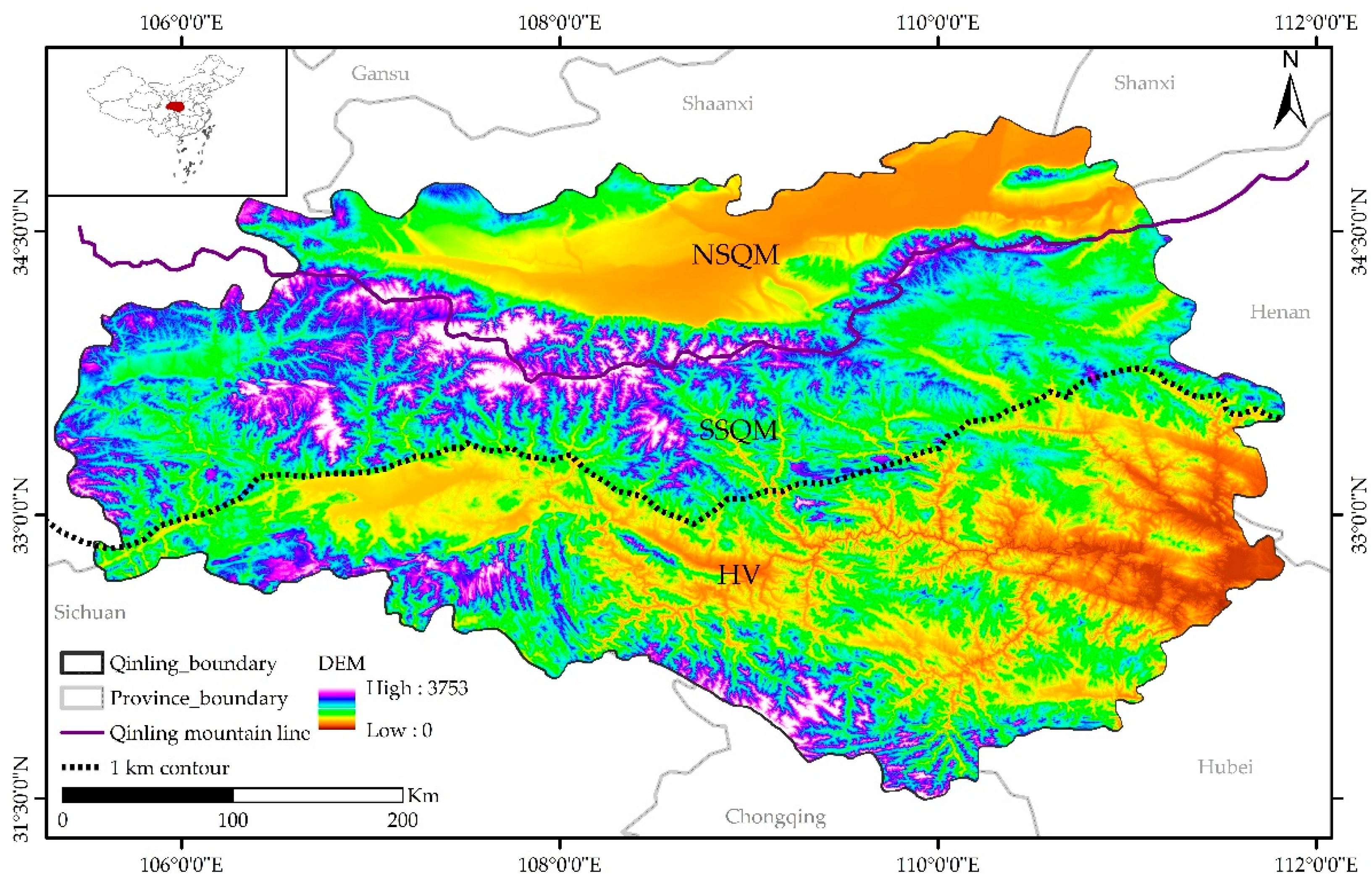
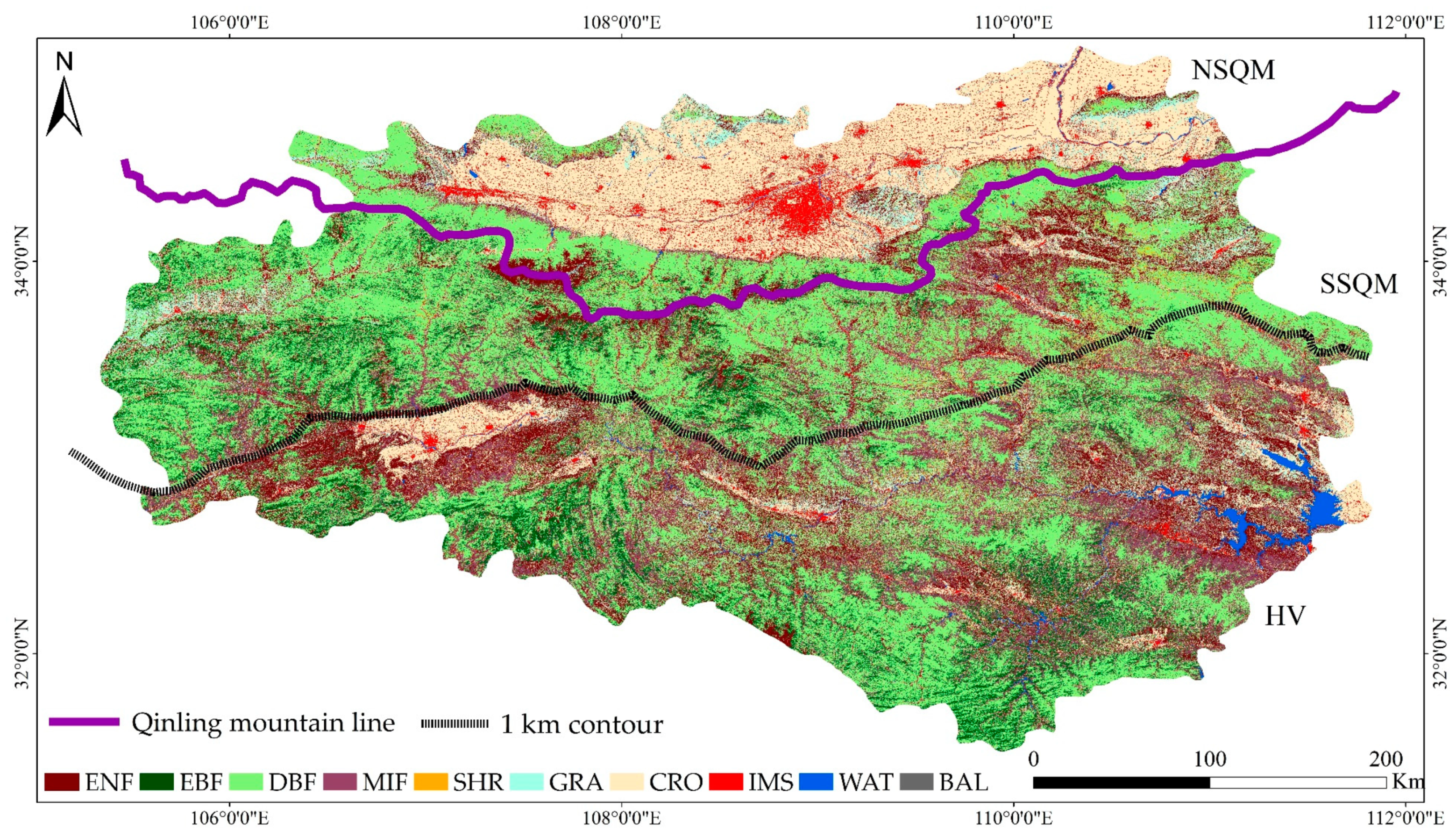
2.1. Study Area

The Qinling Mountains (QMS), located in central China, spans the Gansu, Shaanxi, Hubei, Shanxi, and Henan provinces (Figure 1), covering an area of 148,785 km². It rises gradually from east to west, with a length of ~1600 km and an average altitude of ~2000 m. It divides China’s northern and southern climatic and geographical regions and is the watershed for the Yangtze and Yellow rivers. Due to its unique geographical location and climatic environment, QMS has become a transition zone of natural geography and a sensitive area of climate change and is a hotspot with the richest biodiversity in east Asia. Furthermore, due to the barrier function of its topography, different vegetation types are formed on the north and south slopes. The north slope belongs to the warm temperate semi-humid zone and the forest type is mainly the warm temperate deciduous broadleaved forest. The south slope belongs to the north subtropical humid zone, and the forest type is mainly the north subtropical deciduous broadleaved and evergreen broadleaved mixed forest [16]. The average annual temperature and precipitation of the region are 12−17 °C and 600−1200 mm, respectively.

Recently, the forest resources of QMS have been seriously damaged. Especially in the north slope area, because of the proximity to Xi’an city, deforestation has been more serious. At present, the state has begun to take measures to protect the forest resources in this area, such as the forest ecological project on the north slope and the Qinling National Park project. Therefore, it is vital to obtain accurate forest type distribution information in this area.

2.2. Dataset

2.2.1. Sentinel-2 Remote Sensing Images

Sentinel-2, developed by the European Space Agency (ESA), comprises two identical satellites: Sentinel-2A, launched on 23 June 2015, and Sentinel-2B, launched on 7 March 2017. Sentinel-2 carries a single multispectral instrument (MSI) with 13 spectral bands: four bands at 10 m (blue: 490 nm, green: 560 nm, red: 665 nm, and near infrared (nir: 842 nm), six bands at 20 m (red edge 1: 705 nm, red edge 2: 740 nm, red edge 3: 783 nm, narrow NIR: 865 nm, short wave infrared 1 (swir): 1610 nm, and swir2: 2190 nm), and three bands at a spatial resolution of 60 m (coastal aerosol: 443 nm, water vapor: 940 nm, and swir _cirrus: 1375 nm). We used all images from Sentinel-2A and Sentinel-2B acquired between 1 January 2017, and 31 December 2017, in the study area with cloud cover of less than 30% (a total of 455 images) and 10 m bands (blue, green, red, nir band).

2.2.2. Ancillary Datasets

The ancillary dataset is the Shuttle Radar Topography Mission (SRTM) product (SRTM Plus) provided by NASA JPL, USA at a resolution of 1 arc-s (~30 m). The mosaicking and clipping operations on the SRTM images were first performed using the mosaic and clip function on Google Earth Engine [17]; then, all images were resampled to a 10-m spatial resolution. The slope and aspect features were derived from the clipped images, to assist with forest type classification.

2.2.3. Training and Validation Data

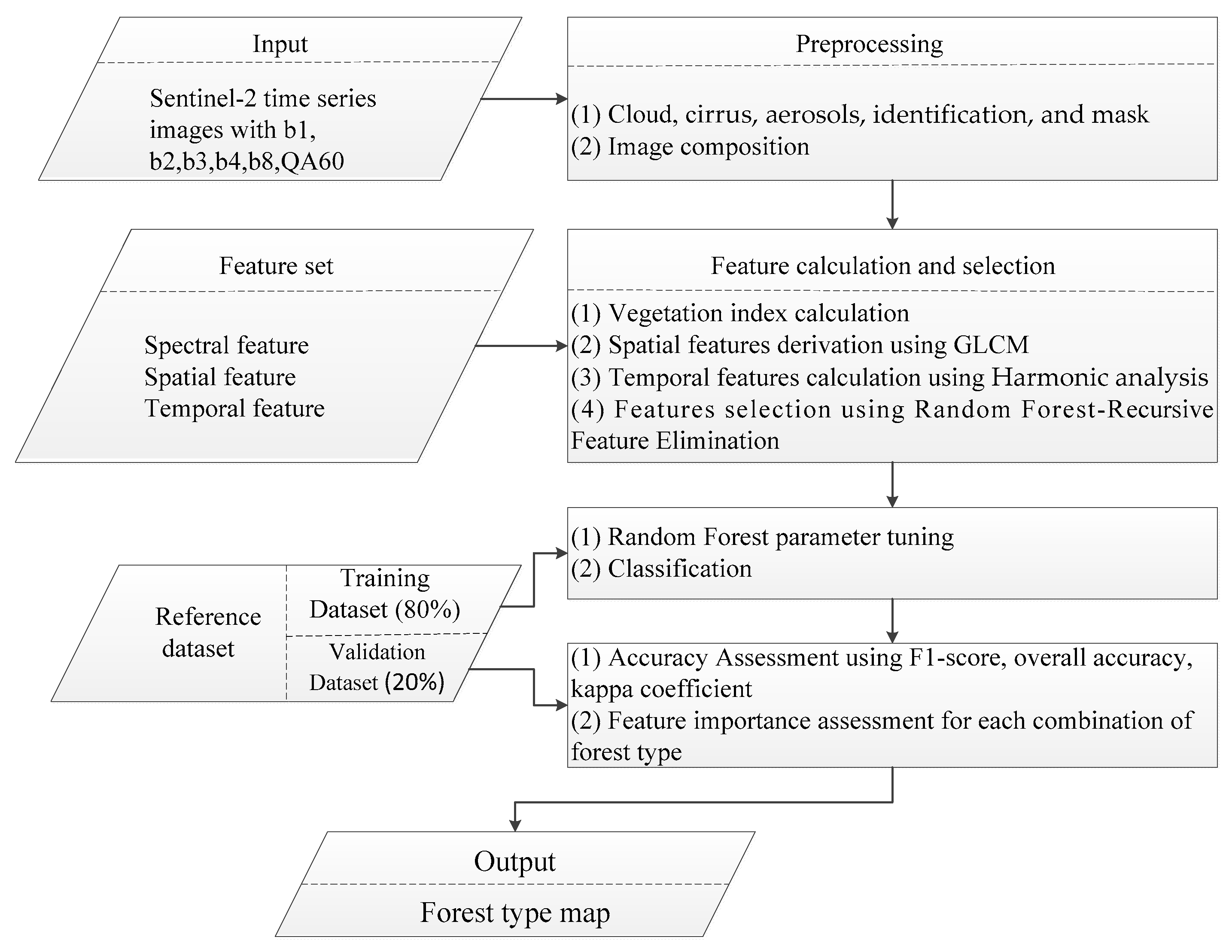
The training and validation data originated from two aspects: field sampling and visual interpretation based on an existing forest inventory map from 2008 (downloaded from the website of China Forest Science Data Center: http://www.cfsdc.org/). We sampled 250 points for the landcover types in the study area between 2013 and 2015. However, due to the steep terrain of the study area, many mountain areas could not be reached, which resulted in uneven sampling of the land cover types. Therefore, we first spatially registered the 2008 forest-type inventory map in ArcGIS 10.3 (ESRI, Redlands, CA, USA), and then used it as a base map to sample the forest type by manual vectorization. To confirm whether these samples changed by 2017, the vectorized samples were superimposed with Google Earth high-resolution images to remove the points with significant changes. Ultimately, 1105 reference data records were acquired, with 80% of the reference data randomly selected in each class as training data, while the rest served for validation (

Table 1. Number of training and validation data for each class.

Land Cover Type	Abbreviation	Training Points	Validation Points
Evergreen needleleaf forest	ENF	124	31
Evergreen broadleaf forest	EBF	128	32
Deciduous broadleaf forest	DBF	184	46
Mixed forest	MIF	104	26
Shrub	SHR	40	10
Grassland	GRD	68	17
Cropland	CRD	104	26
Water	WAR	52	13
Built area	BUA	16	4
Bare land	BAL	64	16

).

2.4. Methodology

The methods used in this study are presented in the flowchart shown in Figure 2, which comprises five steps: (1) preprocessing, (2) feature extraction and selection, (3) supervised classifier training, (4) classification, and (5) evaluation.

2.4.1. Preprocessing

The preprocessing steps are described as follows. (1) Cloud mask: we used Sentinel-2 Band QA60 to identify and mask the flagged cloud and cirrus pixels. The remaining cloud and aerosols were then identified using an aerosol band (Band 1) and were likewise masked. The latter was accomplished using a threshold of Band 1 ≥ 1500 [18]. (2) Image composition: we separated all acquired images in 2017 into two periods and composited them using the following method [19]. One was produced by compositing images from April to September and the other was developed by compositing images from the remaining months. In this way, the images covering the entire area could be generated and the basic phenological characteristics could be retained. This is because most of the vegetation in the QMS started to grow in April, and the deciduous period basically began in early October [20]. The composition results are shown in Figure 3.

2.4.2. Feature Derivation

Spectral Features

The spectral features include two types: one type comprises blue, green, red, and near-infrared bands with 10-m resolution from Sentinel-2 images, and the other type includes several spectral indexes, namely normalized difference vegetation index (NDVI), normalized difference water index (NDWI), modified soil-adjusted vegetation index (MSAVI), and enhanced vegetation index (EVI), derived from the bands. Equations (1)–(4) show their calculation [21,22,23,24,25,26]:

$$\mathrm{NDVI}=\frac{{\rho }_{NIR} - {\rho }_{RED}}{{\rho }_{NIR }+ {\rho }_{RED}},$$

(1)

$$\mathrm{NDWI}=\frac{{\rho }_{NIR} - {\rho }_{GREEN}}{{\rho }_{NIR} + {\rho }_{GREEN}},$$

(2)

$$\mathrm{MSAVI}=\frac{2 \times {\rho }_{NIR} + 1 - \sqrt{(2 \times {\rho }_{NIR} + 1{)}^2- 8 \times \left({\rho }_{NIR} - {\rho }_{RED}\right)}}{2},$$

(3)

$$\mathrm{EVI}=2.5 \times \frac{{\rho }_{NIR} - {\rho }_{RED}}{{\rho }_{NIR} + 6 \times {\rho }_{RED }- 7.5 \times {\rho }_{BLUE} + 1},$$

(4)

where ${\rho }_{NIR}$, ${\rho }_{RED}$, ${\rho }_{GREEN}$, and ${\rho }_{BLUE}$ indicate the reflectance values of the near-infrared (NIR) band (0.8328 mm), red band (0.6646 mm), green band (0.5598 mm), and blue band (0.4924 mm) in the Sentinel-2 MSI sensor.

Spatial Features

The spatial features are represented by texture features, comprising contrast (Con), entropy (Ent), and correlation (Cor), which have been reported to be effective in discriminating forest and other land cover types [11,12,27,28,29,30,31,32]. They were calculated using a gray-level co-occurrence matrix (GLCM); the size of the neighborhood to include in each GLCM was set to four and the kernel was a 3 × 3 square. The formulas of each indicator are shown in Equations (5)–(7):

$$\mathrm{Con}={{\displaystyle \sum }}_{i,j=1}^{N_g}{\left(i-j\right)}^2 \mathrm{GLCM}\left(i,j\right),$$

(5)

$$\mathrm{Ent}={{\displaystyle \sum }}_{i,j=1}^{N_g} {\left(\mathrm{GLCM}\left(i,j\right)\right)}^2,$$

(6)

$$\mathrm{Cor}={{\displaystyle \sum }}_{i,j=1}^{N_g}\frac{\left\{i \times j\right\} \times \mathrm{GLCM}\left(i,j\right) - \left\{{\mu }_x - {\mu }_y\right\}}{{\sigma }_x \times {\sigma }_y},$$

(7)

where $N_g$ is the image gray level, and ${\mu }_x$, ${\mu }_y$ and ${\sigma }_x$, ${\sigma }_y$ are the mean and standard deviations, respectively.

Temporal Features

Harmonic analysis is used to fit to all available observations for each spectral band and NDVI and EVI indices, to extract temporal features, resulting in a set of harmonic features that can describe different growth trajectories or temporal patterns of variation for various forest types, including estimated (1) annual amplitude, (2) phase, and (3) root-mean-square error (RMSE) [31,32,33]. For a series of discrete bands, the harmonics can be defined as shown in Equation (8), and the amplitude and phase can be calculated by Equations (9) and (10), respectively.

$$y_t=a_0 + {{\displaystyle \sum }}_{i=0}^{N-1} \left(a_i cos2\pi f_{i}t+b_i sin2\pi f_{i}t\right),$$

(8)

$$\mathrm{Amplitude}: Am{p}_i=\sqrt[]{a_i^2+b_i^2},$$

(9)

$$\mathrm{Phase}: Ph{a}_i=-\arctan \left(\raisebox{1ex}{$b_i$}\!\left/ \!\raisebox{-1ex}{$a_i$}\right.\right)$$

(10)

where $y_t$ is the time series of a specific band, $f_i$ is the frequency, t is the time, N is the length of the sequence, and $a_0$ is the residual, a white noise sequence, and equal to the average of the time series $y_t$.

All above operations were conducted in Google Earth Engine. Besides the spectral, spatial, and temporal features calculated above, we added some auxiliary features, including elevation and slope. The final feature set list is shown in

Table 2. List of features for forest type classification.

Type	Index	Reference
Spectral feature	blue, green, red, nir, NDVI, EVI, NDWI, MSAVI	[20,21,22,23,24,25]
Spatial feature	blue_contrast, green_contrast, red_contrast, nir_contrast	[26,27,28,29,30,31]
	blue_entropy, green_entropy, red_entropy, nir_entropy
	blue_correlation, gren_correlation, red_correlation, nir_correlation
Temporal feature	blue_amplitude, green_amplitude, red_amplitude, nir_amplitude, NDVI_amplitude, EVI_amplitude	[32,33,34]
	blue_phase, green_phase, red_phase, nir_phase, NDVI_phase, EVI_phase
	blue_RMSE, green_RMSE, red_RMSE, nir_RMSE, NDVI_RMSE, EVI_phase
Ancillary feature	Elevation, aspect, slope	[15,23]

Note: nir represents the near infrared band of image, NDVI represents the normalized difference vegetation index, EVI represents the enhanced vegetation index, NDWI represents the normalized difference water index, MSAVI represents the modified soil-adjusted vegetation index, RMSE represents the root-mean-square error.

.

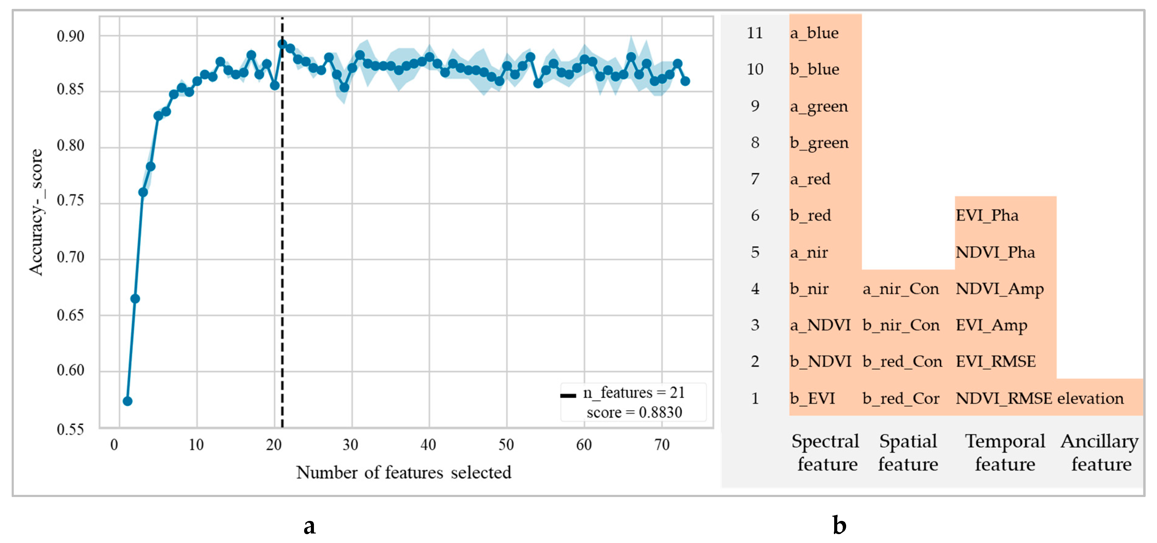
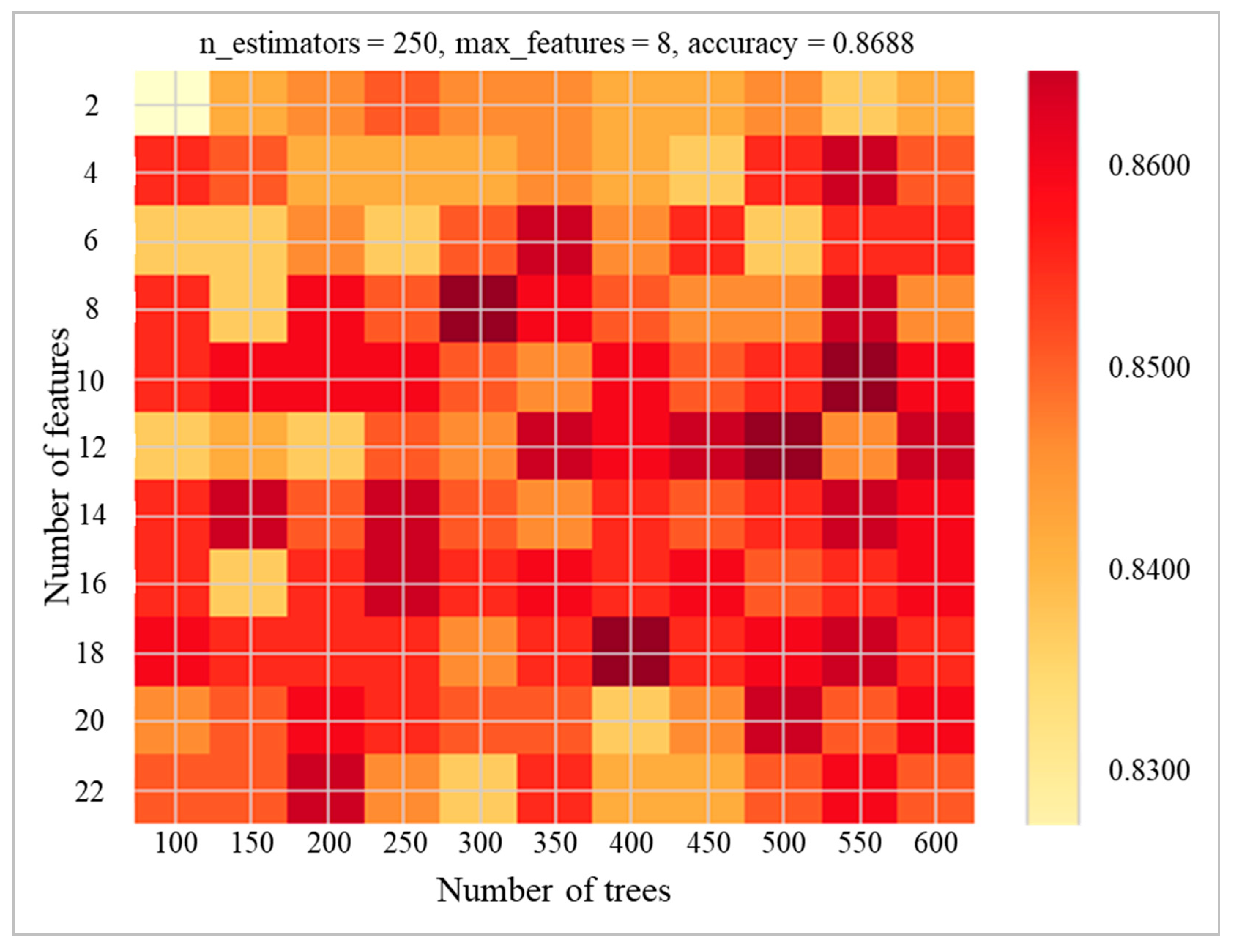
2.4.3. Random Forest Algorithm and Feature Selection

RF is an integrated learning method based on a decision tree, which is combined with many ensemble regression or classification trees [34], and has become increasingly common in remote sensing applications due to its flexible, nonparametric nature and ability to limit overfitting [35,36]. Two important parameters in the RF classifier need to be set up: the number of trees (ntree) and the number of features in each split (mtry). To obtain the optimal parameters, grid search techniques were implemented to optimize the classifier parameters and ensure model fitting using the training data listed in Table 1.

To reduce the redundant information between features and the overfitting problem [37,38], the random forest-recursive feature elimination (RF-RFE) algorithm was used to reduce the number of features. We employed a Python implementation of the RF-RFE algorithm, whose procedure is as follows: (1) training RF model based on the training data and acquiring each feature’s importance according to their classification contribution. (2) Sorting the features from high to low according to their importance. The ranking of features was obtained in this step. (3) Eliminating the least important feature, and then, using the updated features to re-train the RF model and obtain the classification performance using the new feature set. This procedure was run iteratively until the feature set was empty. After running RF-RFE, a list of performance measurement values corresponding to each subset was produced.

2.4.4. Evaluation and Feature Importance Assessment

Evaluation

The evaluation included two parts: (1) assessment of classification mode based on SST features using precision, recall, and F1_score indices, and (2) accuracy assessment of the classified map using overall accuracy (OA), kappa coefficient (KC), producer’s accuracy (PA), and user’s accuracy (UA) calculated through the confusion matrix.

Feature Importance Assessment

Feature importance scores were measured internally by the RF algorithm using the Gini criterion and optimized feature collection. High Gini scores correspond to features that are consistently found more often and higher up in the splits of individual decision trees.

A series of additional RF classifications using this optimized feature set were performed to assess feature importance for the following combinations of forest types: (a) all five classes (for reference), (b) evergreen needleleaf forest paired with evergreen broadleaf forest (ENF vs. EBF), (c) evergreen needleleaf forest paired with deciduous broadleaf forest (ENF vs. DBF), (d) evergreen needleleaf forest paired with shrub (ENF vs. SHR), (e) evergreen broadleaf forest paired with deciduous broadleaf forest (EBF vs. DBF), (f) evergreen broadleaf forest paired with shrub (EBF vs. SHR), and (g) deciduous broadleaf forest paired with shrub (DBF vs. SHR). For each combination of classes, a single RF classifier using data only from the specified classes was applied for training. For example, the ENF vs. EBF feature importance assessment was performed using an RF trained only on pixels from evergreen needleleaf forest and evergreen broadleaf forest points.

3. Results

3.1. SST Feature Set and Classification Result

After executing RF-RFE 20 times, the optimal number of features was obtained, as shown in Figure 4. Figure 4a indicates that in the early stage, the accuracy increased significantly. When the number of features was equal to 21, the accuracy reached its peak. For a greater number of features, the accuracy underwent small fluctuations and showed a downward trend overall. Therefore, the optimal number of features used in forest type classification was 21. Figure 4b presents the 21 specific features. The number of spectral features was the largest, including blue, green, red, nir, NDVI, and EVI from different periods, followed by temporal features, including EVI_Pha, NDVI_Pha, NDVI_Amp, EVI_Amp, EVI_RMSE, and NDVI_RMSE. Spatial features were the least in number, including nir_Con, red_Con, and red_Cor. Using the determined SST feature set, the key parameters of RF were determined (Figure 5). The parameter ntrees was tuned with values ranging from 100 to 600 with intervals of 50, while mtry was set 1 to 11. The parameter combination that yielded the highest testing accuracy was used as the optimal classifier parameter. The highest accuracy was obtained when the number of trees and features were equal to 300 and 4, respectively.

Based on the trained RF and SST feature set, the classification result was output and is presented in Figure 6. The visual result indicates that the forest resources were very rich in QMS. Through statistics based on ArcGIS 10.3 software, the forest accounted for ~74.44% of the total area, which is very similar to the 75% value published by the China Forest Science Data Center. Different forest types exhibited different distribution characteristics. Evergreen broadleaf forest (EBF) was mainly distributed on the central and west regions with high elevation, while DBF was mostly located in the northeast direction.

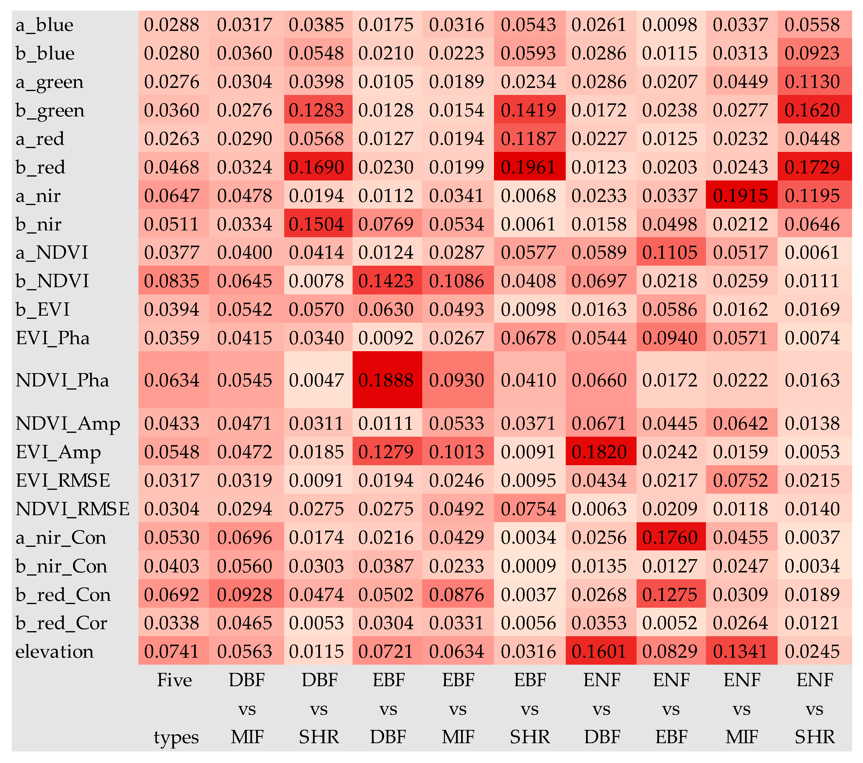
3.2. Feature Importance for Different Forest Type Classification

The results of the feature importance assessment were considerably varied, depending on the types used in training the RF classifier (Figure 7). When the classifier was trained on the full set of the five forest types, the importance of the spectral, spatial, and temporal features was found to be similar, with values between 0.0263 and 0.0835. Among the features, b_NDVI in the spectral feature set had the highest overall importance (0.0835), followed by elevation (0.0741) and b_red_Con (0.0692) in the spatial feature set.

Discrimination in terms of importance among features was more apparent when fewer classes were used in training. For example, only considering deciduous broadleaf forest (DBF) and shrubs (SHR), the importance of b_green, b_red, and b_nir in spectral features was much larger than that of the others. When discriminating between DBF and EBF types, the results were different, and b_NDVI in spectral features and NDVI_Pha and EVI_Amp in temporal features played the most important roles. It was also observed that b_red_Con of spatial (texture) features exhibited the greatest importance in discriminating DBF and mixed forest (MIF), with a value of 0.0928. However, it was not much larger than that of the other features. Furthermore, the elevation apparently acquired a higher importance in differentiating evergreen needleleaf forest (ENF) and DBF, ENF and MIF, which is attributable to the landform of the study area.

3.3. Evaluation of SST-Based RF Classifier and Classification Result

The performance of the SST-based RF classifier is shown in

Table 3. Performance of SST-based random forest (RF) classifier.

Land Cover Type	Precision	Recall	F1 Score
ENF	0.90	0.90	0.90
EBF	0.93	0.84	0.89
DBF	0.83	0.87	0.85
MIF	0.83	0.92	0.87
SHR	0.89	0.80	0.84
GRA	0.81	1.00	0.89
CRO	0.88	0.88	0.88
BUI	0.91	0.77	0.83
WAT	0.80	1.00	0.89
BAR	0.92	0.69	0.79
Average	0.87	0.87	0.87

. The average F1 score was 0.87, which indicated that the model realized a higher performance in forest type classification. The model performed very well for the forest types, the F1 scores were between 0.84 and 0.90, ENF obtained the highest F1 score (0.90), and SHR obtained the lowest F1 score (0.84). For other land cover types, the method also presented acceptable results, especially for grassland (GRA), cropland (CRO), and water (WAT), with F1 scores of 0.89, 0.88, and 0.89, respectively. These results indicated that the SST-based RF model has great advantages in land cover classification; particularly for forest type identification, it shows great application potential.

The classification accuracy was measured using confusion matrices. The user and producer accuracy (UA, PA), the overall accuracy (OA), and the kappa coefficient (KC) were calculated as shown in

Table 4. Confusion matrix for land cover types.

Class	ENF	EBF	DBF	MIF	SHR	GRA	CRO	BUI	WAT	BAR
ENF	28	2	0	1	0	0	0	0	0	0
EBF	1	27	4	0	0	0	0	0	0	0
DBF	2	0	40	4	0	0	0	0	0	0
MIF	0	0	2	24	0	0	0	0	0	0
SHR	0	0	2	0	8	0	0	0	0	0
GRA	0	0	0	0	0	17	0	0	0	0
CRO	0	0	0	0	0	2	23	1	0	0
BUI	0	0	0	0	0	0	1	10	1	1
WAT	0	0	0	0	0	0	0	0	4	0
BAR	0	0	0	0	1	2	2	0	0	11
UA	90.32%	84.38%	86.96%	92.31%	80.00%	100.00%	88.46%	76.92%	100.00%	68.75%
PA	90.32%	93.10%	83.33%	82.76%	88.89%	80.95%	88.46%	90.91%	80.00%	91.67%
OA	86.88%
KC	0.85

Note: UA = User accuracy, PA = Producer accuracy, OA = Overall accuracy, KC = Kappa coefficient.

. The result indicated that the produced forest type and land cover map had an OA of 86.88% (Table 4). Each land cover type included at least one misclassification, except grass land (GRA) and water (WAT). However, regarding forest types, misclassifications were mainly shown between the forest categories. There was no misclassification between forest and other land cover types, indicating that the method was effective for forest extraction. For other land cover types, bare land (BAR) misclassification was the most serious.

The user accuracies for the land cover types varied from 68.75% to 100% and the producer accuracies ranged from 80.00% to 93.10%. Besides IMS and BAR, other land cover types showed producer and user accuracies greater than 80%, which means that these types were obtained with small omission and commission errors and classified with acceptable results. Furthermore, for forest type (ENF, EBF, DBF, MIF, SHR) classification, the most misclassified type was DBF, with more than two points being misclassified as DBF, except in the case of ENF. The most common occurrence of mixed points was EBF, while MIF was the least. However, all forest types exhibited user and producer accuracies greater than 80%, which means that the forest type could be classified well based on the SST-based RF model.

4. Discussion

This study indicated the feasibility and reliability of mapping forest type using SST features and the RF classifier. The method was applied in QMS area situated in the central part of China, and SST features were derived from Sentinel-2 time-series images and optimized using the RF-RFE algorithm. Based on the optimized SST feature set and RF classifier, a forest type map was generated with an OA of 86.88% and a KC of 0.85. This is the first time SST features derived from Sentinel-2 annual time-series images have been integrated for forest type classification.

4.1. Spectral, Spatial, and Temporal Features

Regarding the extraction of SST features, this study provided a universal technique for extracting SST features. This process was developed by integrating the vegetation index, GLCM, and harmonic analysis into a single method. Then, the RF-RFE feature selection algorithm was used to optimize the feature set. For spectral features, we first selected the original bands with the same resolution, which can minimize the effect of spatial resolution. We still selected some vegetation indices to supplement spectral features, including NDVI, NDWI, EVI, and MSAVI. All these indices were demonstrated to be useful for forest type and land cover classification. For example, Liu et al. extracted eight forest types and showed that NDVI has a great impact on forest type discrimination [15]. Luo et al. integrated Moderate Resolution Imaging Spectroradiometer (MODIS) EVI and NDVI data, and successfully extracted five forest types [39]. Spatial features in this study were measured by texture features, calculated by the GLCM method. This method was commonly used in previous studies and obtained acceptable performance. However, after GLCM calculation, a series of indicators reflecting texture characteristics were produced. We chose three indicators, namely contrast, correlation, and entropy, to represent the texture characteristics of the images, all of which played important roles in forest type classification. For example, Wang et al. mapped mangrove species using these contrast, correlation, entropy, and spectral features, demonstrating that correlation can play an important role in forest extraction [26]. Temporal features were derived using harmonic analysis through Fourier transform, which is a powerful tool for temporal pattern analysis. The amplitude, phase, and RMSE images derived from harmonic components can capture the temporal variability of different forest types [30,40]. This provides a reference for our temporal feature extraction. Based on the above three aspects, we constructed the SST feature set. However, correlations between features may exist, and thus, further feature selection is needed for optimization. We compared two commonly used feature selection methods, non-recursive feature elimination (NRFE) and RFE, based on an RF classifier. The results showed that RFE performed better than NRFE. This is consistent with the conclusion of a previous study [26]. Finally, the optimal number of features using the RF-RFE algorithm was found to be 21. This represents a relatively intact and universal technique route integrating SST features for forest type classification.

4.2. Feature Importance

The SST features had a great impact on forest type discrimination. The spectral and temporal feature set was ranked highly in the feature importance analysis (Figure 7), which indicates that they are generally more useful for discriminating among forest types than texture information. An importance analysis indicated that when considering the classification of full forest types, the importance of all features varied slightly; the SST features played a relatively balanced role. When considering different forest type discrimination (e.g., EBF vs. DBF), variation in the importance appeared more apparent among the features. This can better reveal which forest type was more sensitive to which feature. For example, when discriminating evergreen and deciduous forest types, the temporal features (NDVI_Pha, EVI_Amp) acquired higher importance scores. This illustrated that temporal features should be given more consideration in classifying these forest types. When considering classification among evergreen forest types, texture features, including a_nir_Con and b_red_Con, exhibited a more important role. This suggests that texture features are more suitable for identifying ENF and EBF, which is attributable to the differences in leaf structure. When considering separating shrub and other forest types, spectral features, such as green, red, and NIR bands, had the greatest contribution and should be given more consideration. We also tested the influence of each type of feature set on forest type discrimination, and found that using each single feature set (e.g., only spectral features) produced significantly lower accuracy than feature sets that combined SST features. Therefore, the advantage of SST features relied on the combination of features that characterize spectral, spatial, and temporal variability in the reflectance properties. This finding was further supported by the results of feature importance analysis, which demonstrated that all spectral, spatial, and temporal features played an important role in discriminating various forest types.

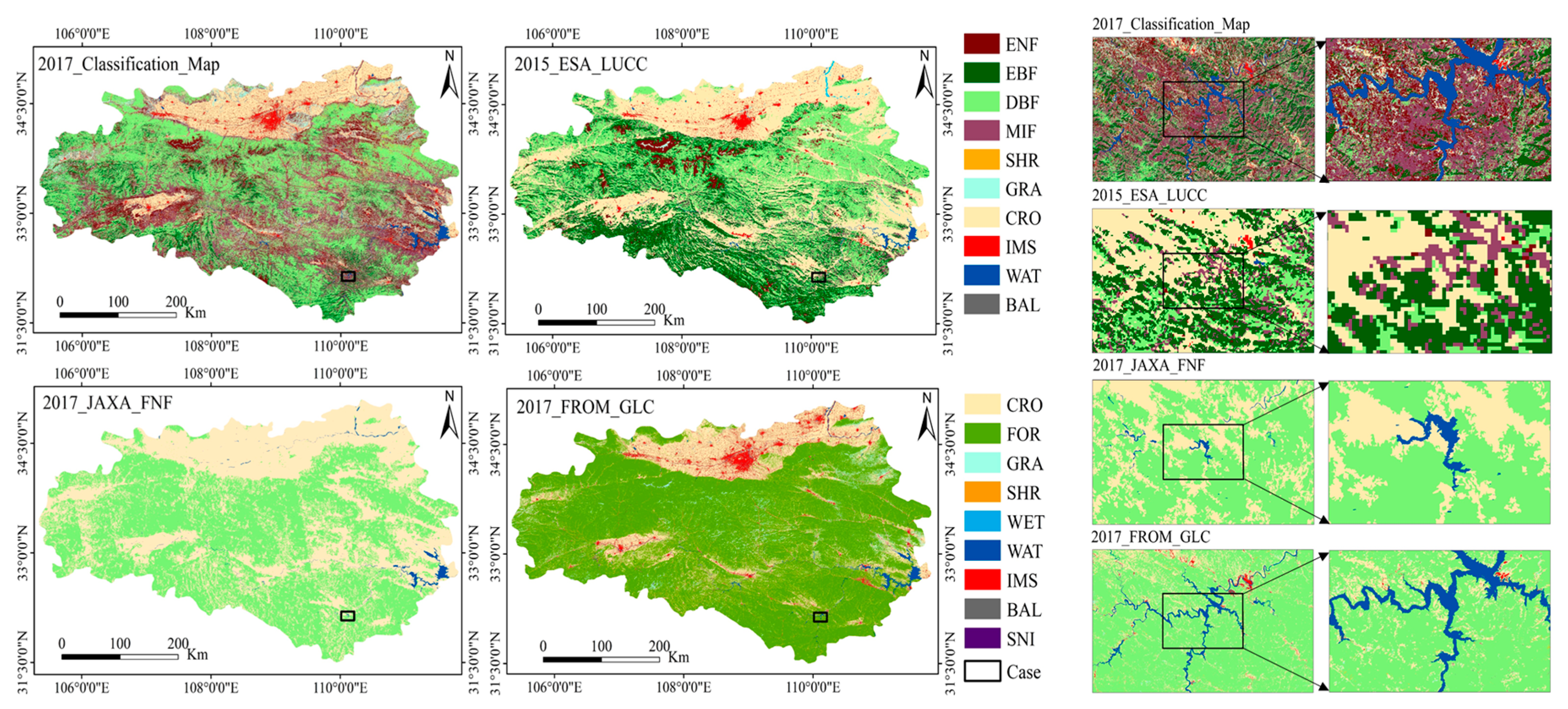
4.3. Comparison with Existing Products

The classification map was acquired using the RF classifier on the optimal SST feature set. The results indicated that the SST-based method was acceptable and reliable with an overall accuracy of 86.88% and a kappa coefficient of 0.85. This result was relatively higher than those of some similar studies. For instance, Yan et al. mapped the ENF, DNF, DBF, MIF, and SHR with an OA of 83.8% and a KC of 0.79, using phenological and spectral features [30]. We also selected three other existing land cover and forest maps to compare with our results: European Space Agency Climate Change Initiative Land Cover (ESA_CCI_LC) product in 2015 (it was the latest one), Japan Aerospace Exploration Agency Forest/Non-Forest (JAXA_FNF) map in 2017, and Finer Resolution Observation and Monitoring Global Land Cover (FROM_GLC) product in 2017. The comparison result is shown in Figure 8, where the classification result has a high spatial consistency with ESA_CCI_LC, JAXA_FNF, and FROM_GLC products on the whole. Meanwhile, there were some significant differences in details, e.g., in the case region of Figure 8. Compared to ESA_CCI_LC, the classification map provided more accurate and abundant information. Compared to JAXA_FNF, not only did our result offer a more accurate forest extent, it also provided forest type information. FROM_GLC in 2017 was also generated using Sentinel-2 images and had a 10-m spatial resolution. Compared to FROM_GLC, the result of this study provided more information about forest types and can be better used in forest management. In general, the forest type map is spatially more consistent than the existing forest cover maps (Figure 8), although some differences still exist. This can be attributed to the different methods and data in use: pixel vs. object-based approach, different types of in situ data, and differences in spatial resolution, e.g., Sentinel-2 vs. Landsat-8 spatial resolution (10 m vs. 30 m, resulting in a minimum mapping unit of 100 m² vs. 900 m²). A near-future regional comparison of pixel- to object-based approaches in the same context can shed further light on the nature of their discrepancies—e.g., statistical vs. environmental.

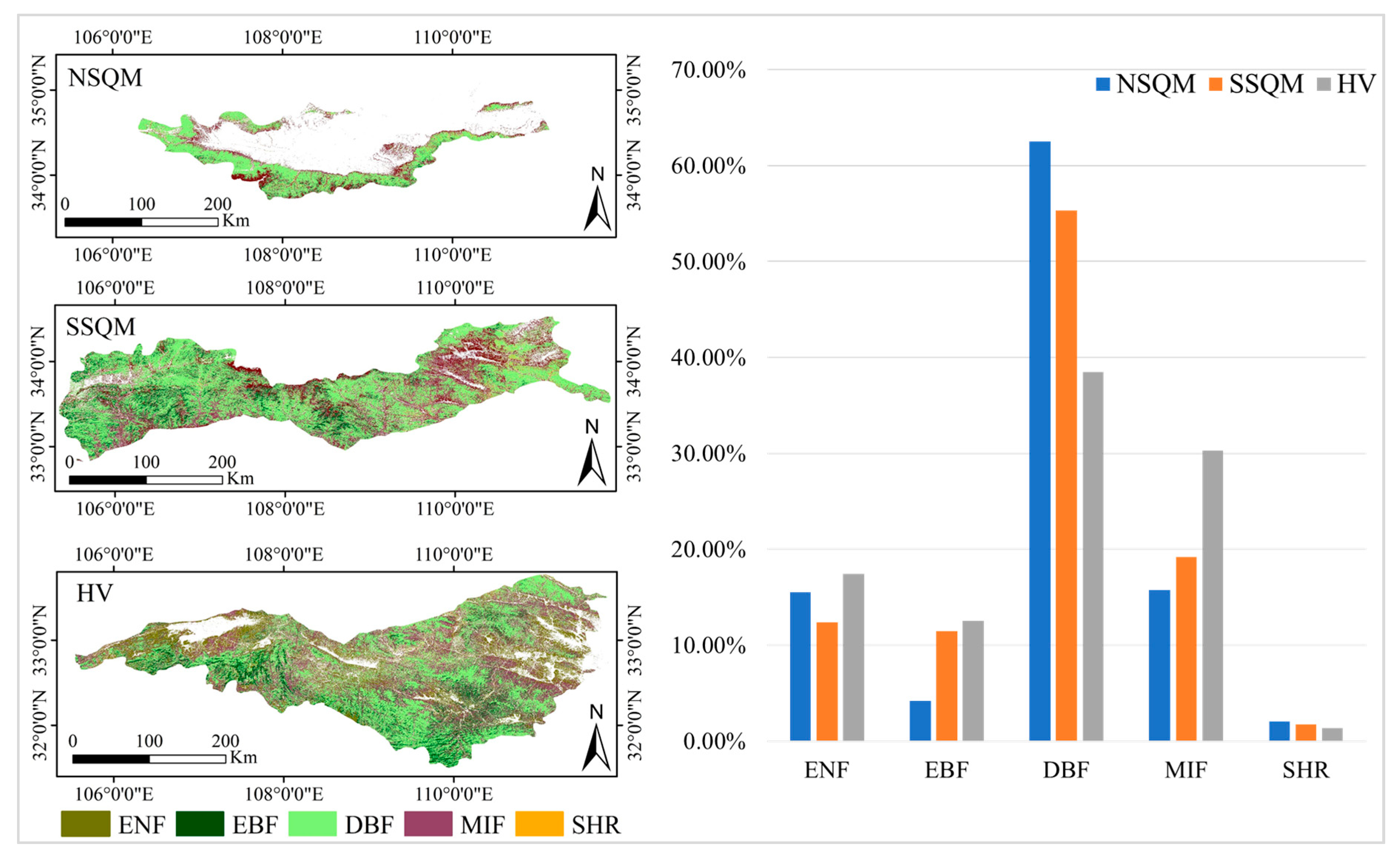
4.4. Forest Type Distribution in QML

QMS is a sensitive area of climate change in China. Due to the barrier function of its topography, different vegetation types are formed on the north and south slopes. Figure 9 shows the distribution and statistic of forest type in different regions. In terms of north slope of QMS (NSQM), the forest resources were mainly distributed near the Qinling mountain line (QML). DBF exhibited the largest area ratio among all forest types, followed by MIF, ENF, EBF, and SHR. This can be explained by the fact that QML exhibits a significant blocking effect on the airflow, making it difficult for the summer ocean currents to penetrate the north. This leads to a dry climate with an average temperature of below 0 °C in January. These factors cause the dominance of DBF in this area. In terms of south slope of QMS (SSQM), the order of the area ratio was the same as that of NSQM, but the ratio of DBF and ENF decreased compared to NSQM, mostly distributed in west and central areas of the region. Meanwhile, EBF and MIF increased significantly and were mostly distributed in central and east parts of the region. This is attributable to the fact that QML blocks the cold wave southward in winter, such that SSQM rarely erodes by cold air and the rivers do not freeze. This leads to an increase in the EBF in SSQM. In terms of Hanjiang valley (HV), the ratio of DBF decreased again and was mainly distributed in the east, while EBF increased continuously and was distributed in the west and southeast. On the other hand, MIF increased significantly and was mostly distributed in the east. This suggests that HV belongs to the subtropical monsoon climate, causing EBF to appear in abundance. These results show that from the north to the east, the forest type shows a significant transition along with climate change and the composition becomes increasingly complex.

This study shows that there is great potential for extracting forest types based on SST features. Experimental results for the five forest types showed that the proposed method achieved acceptable accuracy. However, there are still some limitations that need to be addressed. First, for the data source of multispectral remote sensing images, we selected Sentinel-2 time-series images and limited the bands to blue, green, red, and NIR. This limited the SST features used in the experiment. However, this does not affect the objectives or conclusions. Future study can combine multisource time-series data with a wider spectral range to continue exploring more valuable SST combinations in forest type extraction. Second, given the limitation of reference data, this study could only divide forest types into the five categories of ENF, EBF, DBF, MIF, and SHR. Future research can expand the categories of the reference data and continue to explore the role of SST features in fine forest type extraction, provide basic data for fine management of forest resources, and promote the realization of sustainable management for various forest types in UN SDGs.

5. Conclusions

This paper proposed a forest type classification framework based on SST features and a random forest classifier. This is the first time spectral, spatial, and temporal features derived from Sentinel-2 annual time-series images were integrated for forest type classification. SST features were derived from multispectral time-series images using original bands, vegetation indexes, GLCM, and harmonic analysis methods. Through an example using Sentinel-2 time-series images in the complex forested landscape of Qinling Mountains, China, this method was demonstrated to be robust and reliable. We also found that each forest type had different sensitivities to different kinds of features. Spectral features contribute the most in separating shrub and other forest types, spatial features are more suitable for discriminating evergreen forest types, and temporal features are more useful for differentiating evergreen and deciduous forest and shrub types.

References

1. Masek, J.G.; Hayes, D.J.; Hughes, M.J.; Healey, S.P.; Turner, D.P. The role of remote sensing in process-scaling studies of managed forest ecosystems. For. Ecol. Manag. 2015, 355, 109–123. [Google Scholar] [CrossRef] [Green Version]
2. McKinley, D.C.; Ryan, M.G.; Birdsey, R.A.; Giardina, C.P.; Harmon, M.E.; Heath, L.S.; Houghton, R.A.; Jackson, R.B.; Morrison, J.F.; Murray, B.C. A synthesis of current knowledge on forests and carbon storage in the United States. Ecol. Appl. 2011, 21, 1902–1924. [Google Scholar] [CrossRef] [PubMed] [Green Version]
3. Townshend, J.; Masek, J.G.; Huang, C.Q.; Vermote, E.F.; Gao, F.; Channan, S.; Sexton, J.O.; Feng, M.; Narasimhan, R.; Kim, D.; et al. Global characterization and monitoring of forest cover using Landsat data: Opportunities and challenges. Int. J. Digit. Earth 2012, 5, 373–397. [Google Scholar] [CrossRef]
4. UNSC. Revised List of Global Sustainable Development Goal Indicators, United Nations Statistical Commission. Available online: https://unstats.un.org/sdgs (accessed on 6 July 2017).
5. Fassnacht, F.E.; Latifi, H.; Stereńczak, K.; Modzeleska, A.; Lefsky, M.; Waser, L.T.; Straub, C.; Ghosh, A. Review of studies on tree species classification from remotely sensed data. Remote Sens. Environ. 2016, 186, 64–87. [Google Scholar] [CrossRef]
6. Yan, L.; Jiang, W. Progress in the study of vegetation cover classification of multispectral remote sensing imagery. Remote Sens. Land Resour. 2016, 28, 8–13. [Google Scholar]
7. Zhang, S.F.; Xing, Y.Q.; Abuduaini, A.; Sun, X. Comparison on Forest Type Classification Methods Based on TM Images. Forest Eng. 2014, 30, 18–21. [Google Scholar]
8. Zhang, X.; Zhang, Y.; Liu, L.; Zhang, J.; Gao, J. Remote sensing monitoring of the subalpine coniferous forests and quantitative analysis of the characteristics of succession in east mountain area of Tibetan Plateau—A case study with Zamtange county. Agric. Sci. Technol. 2011, 12, 926–930. [Google Scholar]
9. Sayn-Wittgenstein, L. Recognition of tree species on aerial photographs. In Information Report FMR-X-118; Forest Management Institute: Ottawa, ON, Canada, 1978. [Google Scholar]
10. Franklin, S.E.; Hall, R.J.; Moskal, L.M.; Maudie, A.J.; Lavigne, M.B. Incorporating texture into classification of forest species composition from airborne multispectral images. Int. J. Remote Sens. 2000, 21, 61–79. [Google Scholar] [CrossRef]
11. Mallinis, G.; Koutsias, N.; Tsakiri-Strati, M.; Karteris, M. Object-based classification using Quickbird imagery for delineating forest vegetation polygons in a Mediterranean test site. ISPRS J. Photogramm. Remote Sens. 2008, 63, 237–250. [Google Scholar] [CrossRef]
12. Johansen, K.; Phinn, S. Mapping structural parameters and species composition of riparian vegetation using IKONOS and Landsat ETM+ data in Australian tropical savannahs. Photogramm. Eng. Remote Sens. 2006, 72, 71–80. [Google Scholar] [CrossRef]
13. Gärtner, P.; Förster, M.; Kleinschmit, B. The benefit of synthetically generated RapidEye and Landsat 8 data fusion time series for riparian forest disturbance monitoring. Remote Sens. Environ. 2016, 177, 237–247. [Google Scholar] [CrossRef] [Green Version]
14. Liu, Y.; Gong, W.; Hu, X.; Gong, J. Forest Type Identification with Random Forest Using Sentinel-1A, Sentinel-2A, Multi-Temporal Landsat-8 and DEM Data. Remote Sens. 2018, 10, 946. [Google Scholar] [CrossRef]
15. Xia, Q.; Qin, C.Z.; Li, H.; Huang, C.; Su, F.Z. Mapping Mangrove Forests Based on Multi-Tidal High-Resolution Satellite Imagery. Remote Sens. 2018, 10, 1343. [Google Scholar] [CrossRef]
16. Gao, X.; Bai, H.Y.; Zhang, S.H.; He, Y.N. Climatic change tendency in Qinling Mountains from 1959 to 2009. Bull. Soil Water Conserv. 2012, 32, 207–211. [Google Scholar]
17. Hird, J.N.; DeLancey, E.R.; McDermid, G.J.; Kariyeva, J. Google Earth Engine, Open-Access Satellite Data, and Machine Learning in Support of Large-Area Probabilistic Wetland Mapping. Remote Sens. 2017, 9, 1315. [Google Scholar] [CrossRef]
18. Kaspar, H.; Andreas, H.; Lukas, W. Technical Report; Centre for Development and Environment (CDE) University of Bern: Bern, Switzerland, 2017. [Google Scholar]
19. Xia, H.; Li, A.; Zhao, W.; Bian, J.; Lei, G. Spatiotemporal variations of forest phenology in the Qinling zone based on remote sensing monitoring, 2001–2010. Prog. Geog. 2015, 34, 1297–1305. [Google Scholar]
20. Korhonen, L.; Hadi; Packalen, P.; Rautiainen, M. Comparison of Sentinel-2 and Landsat 8 in the estimation of boreal forest canopy cover and leaf area index. Remote Sens. Environ. 2017, 195, 259–274. [Google Scholar] [CrossRef]
21. Wicaksono, P.; Danoedoro, P.; Hartono; Nehren, U. Mangrove biomass carbon stock mapping of the Karimunjawa islands using multispectral remote sensing. Int. J. Remote Sens. 2016, 37, 26–52. [Google Scholar] [CrossRef]
22. Gitelson, A.A.; Gritz, Y.; Merzlyak, M.N. Relationships between leaf chlorophyll content and spectral reflectance and algorithms for non-destructive chlorophyll assessment in higher plant leaves. J. Plant Physiol. 2003, 160, 271–282. [Google Scholar] [CrossRef]
23. Wolter, P.T.; Mladenoff, D.J.; Host, G.E.; Crow, T.R. Improved forest classification in the northern lake-states using multitemporal Landsat imagery. Photogramm. Eng. Remote Sens. 1995, 61, 1129–1143. [Google Scholar]
24. Maiersperger, T.K.; Cohen, W.B.; Ganio, L.M. A TM-based hardwood-conifer mixture index for closed canopy forests in the Oregon Coast Range. Int. J. Remote Sens. 2001, 22, 1053–1066. [Google Scholar] [CrossRef]
25. Dymond, C.C.; Mladenoff, D.J.; Radeloff, V.C. Phenological differences in tasseled cap indices improve deciduous forest classification. Remote Sens. Environ. 2002, 80, 460–472. [Google Scholar] [CrossRef]
26. Wang, D.; Wan, B.; Qiu, P.; Su, Y.; Guo, Q.; Wang, R.; Sun, F.; Wu, X. Evaluating the Performance of Sentinel-2, Landsat 8 and Pléiades-1 in Mapping Mangrove Extent and Species. Remote Sens. 2018, 10, 1468. [Google Scholar] [CrossRef]
27. Huang, X.; Liu, X.; Zhang, L. A multichannel gray level co-occurrence matrix for multi/hyperspectral image texture representation. Remote Sens. 2014, 6, 8424–8445. [Google Scholar] [CrossRef]
28. Ouma, Y.O.; Tetuko, J.; Tateishi, R. Analysis of co-occurrence and discrete wavelet transform textures for differentiation of forest and non-forest vegetation in very-high-resolution optical-sensor imagery. Int. J. Remote Sens. 2008, 29, 3417–3456. [Google Scholar] [CrossRef]
29. Wang, T.; Zhang, H.; Lin, H.; Fang, C. Textural–spectral feature-based species classification of mangroves in Mai Po nature reserve from Worldview-3 imagery. Remote Sens. 2016, 8, 24. [Google Scholar] [CrossRef]
30. Yan, E.; Wang, G.; Lin, H.; Xia, C.; Sun, H. Phenology-based classification of vegetation cover types in Northeast China using MODIS NDVI and EVI time series. Int. J. Remote Sens. 2015, 36, 489–512. [Google Scholar] [CrossRef]
31. Jakubauskas, M.E.; Legates, D.R.; Kastens, J.H. Crop Identification Using Harmonic Analysis of Time-Series AVHRR NDVI Data. Comput. Electron. Agric. 2002, 37, 127–139. [Google Scholar] [CrossRef]
32. Zhang, X.; Friedl, M.A.; Schaaf, C.B.; Strahler, A.H.; Hodges, J.C.F.; Gao, F.; Reedb, B.C.; Huetec, A. Monitoring Vegetation Phenology Using MODIS. Remote Sens. Environ. 2003, 84, 471–475. [Google Scholar] [CrossRef]
33. Gorelick, N.; Hancher, M.; Dixon, M.; Ilyushchenko, S.; Thau, D.; Moore, R. Google Earth Engine: Planetary-scale geospatial analysis for everyone. Remote Sens. Environ. 2017, 202, 18–27. [Google Scholar] [CrossRef]
34. Breiman, L. Random forests. Mach. Learn. 2001, 45, 5–32. [Google Scholar] [CrossRef]
35. Belgiu, M.; Drăguţ, L. Random forest in remote sensing: A review of applications and future directions. ISPRS J. Photogramm. Remote Sens. 2016, 114, 24–31. [Google Scholar] [CrossRef]
36. Gómez, C.; White, J.C.; Wulder, M.A. Optical remotely sensed time series data for land cover classification: A review. ISPRS J. Photogramm. Remote Sens. 2016, 116, 55–72. [Google Scholar] [CrossRef] [Green Version]
37. Pham, L.T.H.; Brabyn, L. Monitoring mangrove biomass change in Vietnam using spot images and an object-based approach combined with machine learning algorithms. ISPRS J. Photogramm. Remote Sens. 2017, 128, 86–97. [Google Scholar] [CrossRef]
38. Gregorutti, B.; Michel, B.; Saint-Pierre, P. Correlation and variable importance in random forests. Stat. Comput. 2017, 27, 659–678. [Google Scholar] [CrossRef]
39. Luo, C.Q.; Lin, H.; Sun, H.; Wu, Z.S. Based on MODIS image large-scale forest resources information extraction method. J. Central South. Univ. For. Tech. 2015, 11, 21–26. [Google Scholar]
40. Pasquarella, V.J.; Holden, C.E.; Woodcock, C.E. Improved mapping of forest type using spectral-temporal Landsat features. Remote Sens. Environ. 2018, 210, 193–207. [Google Scholar] [CrossRef]
Figure 1. Location of the study site in China and its distribution of evaluation. The 1 km contour represents the contour line located in the south of the Qinling mountain line with an elevation of 1 km. NSQM represents the north slope of the Qinling Mountains (QMS), located in the north of Qinling mountain line. SSQM represents the south slope of QMS, located between the south of Qinling mountain line and 1 km contour. HV represents Hanjiang valley, located in the south of 1 km contour.
Forests 10 00559 g001
Figure 2. Methodological workflow of the study.
Forests 10 00559 g002
Figure 3. Composition result from April to September (a) and October to March (b).
Forests 10 00559 g003
Figure 4. Feature selection using random forest-recursive feature elimination (RF-RFE) algorithm. (a) Optimal number of features; (b) spectral-spatial-temporal (SST) feature set obtained. n_features represents the number of features used in the RF-RFE algorithm. In (b), a_ and b_ represent different periods. For example, a_blue represents the blue band from the image composited between April and September.
Forests 10 00559 g004
Figure 5. Value range of ntree and mtry, and the accuracy of different combinations of ntree and mtry. Darker colors represent higher accuracies. ntree represents number of trees and mtry represents the number of features.
Forests 10 00559 g005
Figure 6. Classification map based on SST random forest classifier. Each color corresponds to an individual forest or land cover type, including Evergreen needleleaf forest (ENF), Evergreen broadleaf forest (EBF), Mixed forest (MIF), Shrub (SHR), Grassland (GRA), Cropland (CRO), Impervious surface (IMS), Water (WAT), and Bare land (BAL).
Forests 10 00559 g006
Figure 7. Feature importance score. Feature importance for discriminating various combinations of forest types, where a and b represent the composited image of April to September and September to April, respectively; for example, a_blue corresponds the blue band from the composited image of April to September.
Forests 10 00559 g007
Figure 8. Comparison of the classified map in 2017, European Space Agency Climate Change Initiative Land Cover (ESA_CCI_LC) in 2015, Japan Aerospace Exploration Agency Forest/Non-Forest (JAXA_FNF) in 2017, and Finer Resolution Observation and Monitoring Global Land Cover (FROM_GLC) in 2017 in a case region.
Forests 10 00559 g008
Figure 9. Composition and distribution of forest type in NSQM, SSQM, and HV. NSQM represents the north slope of QMS; SSQM represents the south slope of QMS; and HV represents Hanjiang valley located in the south region of 1 km contour line.
Forests 10 00559 g009