Contribution Analysis of the Spatial-Temporal Changes in Streamflow in a Typical Elevation Transitional Watershed of Southwest China over the Past Six Decades

Abstract

Attribution analyses on streamflow variation to changing climate and land surface characteristics are critical in studies of watershed hydrology. However, attribution results may differ greatly on different spatial and temporal scales, which has not been extensively studied previously. This study aims to investigate the spatial-temporal contributions of climate change and underlying surface variation to streamflow alteration using Budyko framework. Jiangling River Watershed (JRW), a typical landform transitional watershed in Southwest China, was chosen as the study area. The watershed was firstly divided into eight sub-basins by hydrologic stations, and hydrometeorological series (1954–2015) were divided into sub-intervals to discriminate spatial-temporal features. The results showed that long-term tendencies of hydrometeorological variables, i.e., precipitation (P), potential evapotranspiration (E₀), and runoff depth (R), exhibited clear spatial patterns, which were highly related to topographic characteristics. Additionally, sensitivity analysis, which interpreted the effect of one driving factor by unit change, showed that climate factors P and E₀, and catchment characteristics (land surface parameter n) played positive, negative, and negative roles in R, according to elastic coefficients (ε), respectively. The spatial distribution of ε illustrated a greater sensitivity and heterogeneity in the plateau and semi-humid regions (upstream). Moreover, the results from attribution analysis showed that the contribution of the land surface factor accounted for approximately 80% of the R change for the entire JRW, with an obvious spatial variation. Furthermore, tendencies of the contribution rates demonstrated regulations across different sub-regions: a decreasing trend of land surface impacts in trunk stream regions and increasing tendencies in tributary regions, and vice versa for climate impacts. Overall, both hydrometeorological variables and contributions of influencing factors presented regularities in long-term tendencies across different sub-regions. More particularly, the impact of the primary influencing factor on all sub-basins exhibited a decreasing trend over time. The evidence that climate and land surface change act on streamflow in a synergistic way, would complicate the attribution analysis and bring a new challenge to attribution analysis.

1. Introduction

Addressing the issue of water resources requires knowledge of the factors, which drive hydrologic changes and the related effects on local river flow. Generally, climate variation and land surface characteristics are considered as the two major contributors to the changing streamflow in many regions of the world [1,2,3,4]. Climate fluctuations mainly affect streamflow through precipitation (P) and potential evapotranspiration (E₀) variations. Changes in land surface properties, including the topography, vegetation coverage, land use characteristics, reservoir operations, etc., lead to hydrologic variation by changing the streamflow generation and confluence mechanisms. Climate change combined with land surface features have triggered remarkable changes in hydrological processes which have further caused serious water resources problems [5,6]. Therefore, comprehending and distinguishing the relative impacts of climate change and land surface features on runoff is essential to adapting water resource management and soil and water conservation projects, especially under the conditions of global warming and intensive human activities [7,8,9,10,11].

There are three commonly used methods, with both merits and drawbacks, for quantitatively distinguishing the impacts of climate change and land surface factors on streamflow. Paired catchment experiments, useful for evaluating the mechanism of the soil-vegetation-atmosphere interaction, are often restricted to a small scale and lacked of long-term observations [12,13,14,15,16]. Physical-based hydrologic models, e.g., Hydrological Simulation Program-Fortran (HSPF), Soil and Water Assessment Tool (SWAT), and MIKE System Hydrological European (MIKE SHE) model, embody strong advantages to compute physical processes and quantify contributions of driving factors [17,18]. This processes-based and parameter-dependent approach generally requires well-observed data on the hydrology, climate, and landscape, and comes along with a certain degree of uncertainty [19,20,21]. Statistical methods, e.g., the double mass curve, flow duration curve, and multi-statistical regression model, are relatively simple and require less data, which often lack physical significance [22,23,24,25]. Among the statistical methods, the Budyko hypothesis-based method has demonstrated a strong interpretation of the hydrological mechanism [26,27]. In the Budyko hypothesis, the relationship between streamflow and key driving factors, i.e., precipitation (P) and mean evapotranspiration (E), is assumed to be monotonic [26], and the sensitivity of runoff is related to different climatic variables to separate the contributions of each variable [28]. Further, a catchment property parameter, referring to the combined influence of terrain, soil, vegetation, land use, and human activities, is introduced in Budyko functions to denote the effect of underlying surface characteristics and forms the diversification of Budyko equation [27,29,30,31,32]. With diversified forms, the Budyko hypothesis-based methods have been extensively used to attribute hydrological changes. For instance, Zhou et al. [33] analyzed the global pattern of hydrological response to landcover and climate change using the Budyko hypothesis-based equation with a watershed characteristics parameter w improved by Fu [27]. Shen et al. [34] applied another form of Budyko equation with a catchment parameter n [31] to quantify runoff variation in 224 catchments across China.

Recently, the responses of streamflow to changing climate and land surface characteristics are well documented [18,33,35,36]. However, attribution results may differ greatly at different spatial and temporal scales, which has not been sufficiently studied in most studies of watershed hydrology. On the one hand, driving factors are usually considered to act evenly over the whole watershed and, thus, variations within the study area are neglected. Actually, a watershed, especially a large one, is wide in territory with various climate types, vegetation coverage, topographies, urbanization intensities, and population densities [37]. Impacts of driving factors on streamflow are also shifting from one tributary basin to another [38,39]. Therefore, it is necessary to evaluate the fractional contributions at a sub-basin scale. On the other hand, contribution fractions of driving factors are also time-varying [40,41]. To address the variation of contribution rates at temporal scale, the detection of breakpoints of hydrometeorological time series are critical. With different breakpoints, conclusions or viewpoints on fractional contributions can sometimes be different, which may lead to a misunderstanding of hydrological processes [19,42]. For instance, the meteor-hydrological characteristics in prior impacted period represents original conditions of a watershed. Thus, the determination of unaffected period and the detection of division point determines the assessment of meteor-hydrological elements’ alteration and further effects the evaluation of hydrological attribution. Hence, reasonably dividing the whole watershed into sub-basins and separating long-term time series into sub-intervals are important for acquiring more reliable results [43,44,45]. Moreover, few studies have concentrated on the spatiotemporal heterogeneity of accurate effects on a catchment scale, which would provide critical points in comprehensively analyzing contribution partitions and interacting mechanisms of driving factors in hydrological processes.

The upper region of the Yangtze River is geographically located in the first terrain transition zone of China, with a distinguished change of topography gradient and corresponding climate zones, soil types, and vegetation covers. In the mid-20th century, this region faced problems of deforestation, grassland degradation, water pollution, water shortage, etc. [46,47]. Afterwards, a series of eco-restoration projects were implemented in this area to improve the hydro-ecological environment, such as the Natural Forest Protection Program in 1998, Grain for Green Project in 1999, etc. These measures considerably changed the watershed features and further affected the hydrological systems [17,48]. The Jialing River, as the largest tributary in the upper reaches of the Yangtze River, is a typical watershed characterized by spatially varied climate, landform, and landcover conditions. More concretely, the upstream regions with a higher altitude and drier climate are mainly covered by grass and forest. Meanwhile, the low-lying and humid middle and downstream regions are mostly cultivated land, which has experienced pervasive urban expansion and intensive anthropic disturbances in recent years. As a result of the spatiotemporally varied impacts, streamflow in this basin has exhibited a remarkable decreased tendency over the last six decades [47], leading to a contradiction between the supply and demand of water resources. Therefore, it is arguably vital to quantitively partition the driving factors’ impact on streamflow variation in the Jialing River Watershed (JRW), particularly on a spatiotemporal scale. More seriously, the impact of the two driving factors on runoff in a watershed does not occur in isolation but in a synergistic way, in which, climate, vegetation, and elevation may interact and influence one another, leading to a more complicated problem in watershed management [49]. Therefore, we are also concerned with the above potential reasons for the regularity of the temporal-spatial variation, which is of profound significance for rationally regulating and managing basin water resources.

Based on the above considerations, the scientific objectives of this paper that we are attempting to address are (1) how have the streamflow and driving factors varied both spatially and temporally over the last 62 years in the JWR? (2) At a spatial scale, what are the fractional contributions of driving factors all over the JWR, as well as in the interior of the watershed, which are characterized by distinct variation of climate and topography features? (3) At a temporal scale, have the fractional contributions of driving factors remained constant over the last six decades? If not, what is the tendency of the contribution rates? Finally, we tried to figure out potential reasons for the temporal-spatial heterogeneities as well as the way the driving factors act on the generation of streamflow. The present study involves contribution analyses, by using Budyko-hypothesis framework, across distinct sub-spatial areas and different sub-temporal intervals that may not have been well-considered in previous literature. Meanwhile, a discussion on the way the potential reasons act on streamflow can provide useful information for water resource management and comprehensive watershed harnessing in the Upper Yangtze River.

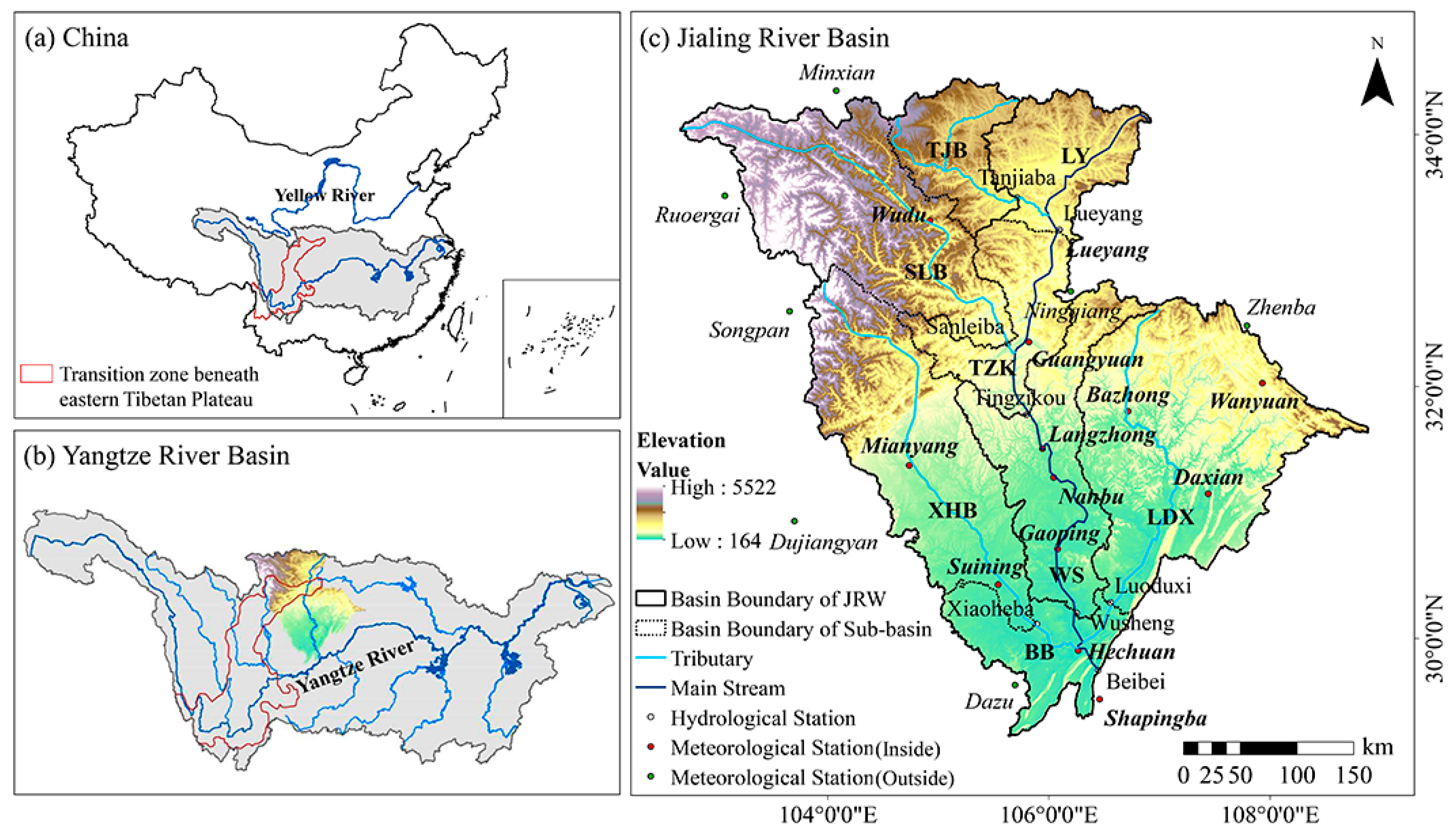
2. Study Area and Data

The Jialing River is a first-order tributary of the Yangtze River and empties into the upper reaches of the Yangtze River from the upstream of the Three Gorges Dam. The JRW spans 29°17′30′′–34°28′11′′ N and 102°35′36″–109°01′08″ E and covers an area of 1.6 × 105 km². Since the whole watershed crosses over the northern part of the transition zone beneath the eastern Tibet Plateau, the terrain has several distinct topographic gradients, namely, plateaus in the northwest, mid-low mountains in the north, hilly regions in the middle-east, and plain regions in the south (Figure 1), with a total height difference of over 5000 m and an average gradient of 2.05‰. The JRW is located in a subtropical monsoon climate region with an average temperature of 16–18 °C. The mean annual precipitation is approximately 1000 mm and gradually decreases from the south to north. More than 60% of the annual precipitation falls between May and September. The Jialing River has the largest sediment concentration in the upper region of the Yangtze River and is an important source of floodwater and sediment for the Three Gorges Reservoir Area. The annual mean runoff and sediment load at Beibei hydrologic station, the hydrology control station of the JRW, is 655.2 × 108 m³ year⁻¹ and 0.967 × 108 t year⁻¹ (1956–2015), respectively, according to the Changjiang Sediment Bulletin. In the past decades, anthropogenic activities have severely interfered with the hydrological cycle and ecological system. Long-term deforestation during the mid-20th century has led to a decrease of vegetation cover and severe soil and water loss, while sustained afforestation activities and ecological restoration measures were undertaken prior to the 1980s, resulting in a dramatic change in land use in the upper Yangtze River. In recent years, the ineluctable urban development and population expansion, dam construction, agricultural irrigation, and water withdrawal have had a non-negligible impact on hydrological processes.

Annual observed discharges in 1954–2015 at four hydrological stations (Wusheng, Beibei, Xiaoheba, and Luoduxi) and annual observed discharges during 1960–2000 (2009) for four other stations (Sanleiba, Tanjiaba, Lueyang, and Tingzikou) were obtained from the Changjiang Water Resource Commission of the Ministry of Water Resources of China. The whole JRW was then partitioned into eight sub-basins by the eight stations, which were located at the outlet of each sub-basin (Figure 1). The designation of these sub-regions was abbreviated as TJB, LY, SLB, TZK, XHB, WS, LDX, and BB, according to the names of the gauging stations (Figure 1). Composited basin MRW (encompasses sub-basins of TJB, LY, SLB, TZK, and WS), as a middle-sized basin, was also investigated. Due to the connection of the river network, four sub-basins (LY, TZK, WS, and BB) were dependent, while the remaining four (SLB, TJB, XHB, and LDX) were independent, in the hydrological process. Note that the basic hypothesis of the Budyko method is that all the regions should satisfy the water balance equation on a long-term time scale. The runoff volume and runoff depth of the above dependent sub-basins, take TZK for example, were calculated by the difference between streamflow records of the outlet station (Tingzikou station) and inlet stations (Sanleiba station and Lueyang station).

Twenty meteorological stations with continuous daily records, i.e., precipitation, air temperature, wind speed, relative humidity, and sunshine hours, from 1954–2015 in and around the JRW, were obtained from the China Meteorological Data Service Center (http://data.cma.cn). The daily potential evapotranspiration (E₀) was estimated using the FAO56 Penman–Monteith method. The annual precipitation (P) and E₀ were then derived according to the daily data. Annual climatic variables in each sub-basin were estimated according to the following workflow: (1) the Kriging algorithm in ArcGIS (Environmental Systems Research Institute, Redlands, CA, USA) was adopted to interpolate meteorological station-based variables into the entire study area, which were stored in a grid format with a resolution that was consistent with other spatial data, e.g., DEM; (2) the mean of climate variables of all grids that were confined by the sub-basin boundary was calculated, and sub-basin based meteorological variables were then derived.

3. Methodology

3.1. Framework of Analysis

In this study, sensitivity and attribution analyses based on Budyko equations were carried out to quantify the climate change and land surface disturbance to streamflow alteration. Runoff alteration caused by climatic factors can be directly estimated by P and E₀, while the left portion caused by land surface interference was estimated by watershed character parameter n. Before carrying out the Budyko strategy, it is fundamentally important to look into the temporal-spatial features of meteorological and hydrological generations in JRW. Therefore, the strategy of the methodology is: (1) detect the trend and abrupt change points by the Mann–Kendall test, Sen’s slope estimator, and Pettitt test, which help look into the spatiotemporal variation features of hydrometeorological elements and divide the time series into prior- and post-impacted stages in a reasonable manner; (2) quantify the relationship between streamflow and its influencing factors by means of sensitivity analysis. Herein, the elastic coefficients will be investigated since they not only provide an illustration of the runoff response to unit change of P, E₀, and catchment properties parameter n, but also essentially enhance our understanding of the contribution calculation; and (3) conduct attribution analysis on both space and temporal scales with the Budyko hypothesis according to the complementary relationship of elastic coefficient of precipitation and potential evapotranspiration proposed by Zhou et al. [50].

3.2. Trend and Abrupt Change Detection

The Mann–Kendall test, Sen’s slope estimator, and Pettitt test are commonly combined and used when detecting tendency and abrupt changes of hydrometeorological generation. The nonparametric Mann–Kendall test has been widely used to establish an effective capability of identifying the monotonic tendency of hydrometeorological series without requiring normality or linearity [51,52]. For a time-series X with n samples, the variable S is constructed as follows:

$$S={\displaystyle \sum _{i=1}^{n-1}{\displaystyle \sum _{j=i+1}^n\mathrm{sgn}\left(x_i-x_j\right)}}$$

(1)

where x_i and x_j are the sequential data values in year i and j, i > j; n is the length of the series; and $\mathrm{sgn}(x_i-x_j)$ is equal to 1, 0, or −1 if x_i is more than, equal to, or less than x_j, respectively.

The test statistic Z_c is defined by:

$$Z_c=\left|\begin{array}{c}\frac{S-1}{\sqrt{V\mathrm{ar}\left(\mathrm{S}\right)}}\\ 0\\ \frac{S+1}{\sqrt{V\mathrm{ar}\left(\mathrm{S}\right)}}\end{array}\begin{array}{c}\\ \\ \end{array}\begin{array}{c}S>0\\ S=0\\ S<0\end{array}\right|$$

(2)

When $\left|Z_c\right|>Z_{1-\alpha /2}$, the null hypothesis is rejected and the sequence has a significant trend. α is the significance level of the test, and sgn(θ) is equal to 1, 0, or −1 if θ is greater than, equal to, or less than zero, respectively.

Sen’s slope index represents the trend of monotonous variation and data changes in per unit time, which is simple and rational as a supplementary unbiased estimator in the Mann–Kendall test [53,54]. The slope of the trend is estimated as follows:

$$\beta =median\left[\frac{\left(x_j-x_i\right)}{\left(j-i\right)}\right],\left(\forall j<i,1\le j\le i\le n\right)$$

(3)

A positive value of β indicates an upward trend and a negative value of β indicates a downward trend.

The non-parametric Pettitt test focuses on the detection of the breaking point with a significance test. The result provides rational stage division which is essential for attribution analysis [55]. The statistic is given as follows:

$$U_{t,n}=U_{t-1,n}+{\displaystyle \sum _{j=1}^n\mathrm{sgn}\left(x_i-x_j\right)},\left(t=2,\dots ,n\right)$$

(4a)

$$k_t=ma{x}_{1\le t\le n}\left|U_{t,n}\right|$$

(4b)

where $\mathrm{sgn}(x_i-x_j)$ is the same as mentioned in Equation (1). The most significant breaking point k_t is determined by the maximum value of |U_{t, n}|.

$$\rho =2\exp \left[-6k_t{}^2/\left(n^3+n^2\right)\right]$$

(5)

The specific significance level in this study is set at 0.05. If ρ ≤ 0.05, the null hypothesis is rejected and the year t is the first order breakpoint with an approximate significance probability of 95%.

3.3. Sensitivity of Runoff Based on the Mezentsev–Choudhury–Yang Equation

For a closed catchment, the water balance equation can be written as [32,56]:

$$R=P-E-\Delta S$$

(6)

where R is the mean annual runoff (mm), P is the mean annual precipitation (mm), and E is the mean annual evaporation (mm), and $\Delta S$ is the variation of catchment water storage.

For long-term periods, longer than 5–10 years, at a catchment scale, the change in soil water content is negligible and the catchment water balance equation is simplified as follows [57,58]:

$$R=P-E$$

(7)

Budyko’s hypothesis states that E is determined by available water and energy at a basin scale based on the water-energy balance [26]. The Mezentsev–Choudhury–Yang function [29,30,31] derives this theory with a consideration of catchment characteristics in the form of:

$$E=\frac{P{E}_0}{{\left(P^{\mathrm{n}}+E_0{}^n\right)}^{1/n}}$$

(8)

where E₀ is the mean annual potential evaporation and the daily value is estimated using the FAO56 Penman–Monteith method [59]. Parameter n is considered to represent catchment characteristics relating to catchment topography, vegetation cover, and other potential factors influencing the water balance and cycle [39,60]. Additionally, P and E₀ are independent of one another in Equation (8).

The FAO56 Penman–Monteith equation [59] is given by:

$$E{T}_0^{}=\frac{0.408\Delta (R_n^{}-G)+\gamma \frac{900}{T+273}{u}_2(e_s-e_a^{})}{\Delta +\gamma (1+0.34u_2)}$$

(9)

where ET₀ represents reference evapotranspiration (mm day⁻¹), R_n represents net radiation at the crop surface (MJ m⁻² day⁻¹), G represents soil heat flux density (MJ m⁻² day⁻¹), T represents mean daily air temperature (°C), u₂ represents wind speed at a 2 m height (m s⁻¹), e_s represents saturation vapor pressure (kpa), e_a represents actual vapor pressure (kpa), e_s−e_a saturation vapor pressure represents deficit (kpa), Δ slope represents the vapor pressure curve (kpa °C⁻¹), and γ represents the psychrometric constant (kpa °C⁻¹).

Combining Equation (7) and Equation (8) generates the following:

$$R=P-\frac{P{E}_0}{{\left(P^n+E_0{}^n\right)}^{1/n}}$$

(10)

Assuming that P and E₀ are independent variables and that both P and E₀ are independent of n in Equation (7), the total differential of R based on the Budyko framework can be written as follows:

$$dR=\frac{\partial R}{\partial P}dP+\frac{\partial R}{\partial E_0}d{E}_0+\frac{\partial R}{\partial n}dn$$

(11)

The concept of using streamflow elasticity to analyze the sensitivity of runoff to climate change was initially introduced by Schaake [28], in which the elasticity of runoff is defined as:

$${\epsilon }_P=\frac{dR/R}{dP/P},{\epsilon }_{E_0}=\frac{dR/R}{d{E}_0/E_0},{\epsilon }_n=\frac{dR/R}{dn/n}$$

(12)

where ${\epsilon }_P$, ${\epsilon }_{E_0}$, and ${\epsilon }_n$ represent the P, E₀, and n elasticity of runoff, respectively, representing ε% change of R induced by a 1% increase of P (E₀, n).

Re-arranging the terms in Equation (10), we can derive the following:

$$\frac{dR}{R}={\epsilon }_P\frac{dP}{P}+{\epsilon }_{E_0}\frac{d{E}_0}{E_0}+{\epsilon }_n\frac{dn}{n}$$

(13)

3.4. Contributions of Climate Change and Catchment Characteristics to Runoff

According to the independence of P and E₀ in Equation (8), Zhou et al. [50,61] proposed the complementary relationship of ${\epsilon }_P$ and ${\epsilon }_{E_0}$ that the sum of ${\epsilon }_P$ and ${\epsilon }_{E_0}$ is equal to unity:

$$\frac{dR/R}{dP/P}+\frac{dR/R}{d{E}_0/E_0}=1$$

(14)

Equation (14) can be transformed as:

$$R=P\frac{dP}{dR}+E_0\frac{d{E}_0}{dR}$$

(15)

Thus, change of runoff can be calculated as follows:

$$dR=\frac{\partial R}{\partial P}dP+\frac{\partial R}{\partial E_0}d{E}_0+Pd\left(\frac{\partial R}{\partial P}\right)+E_{0}d\left(\frac{\partial R}{\partial E_0}\right)$$

(16)

Zhou et al. [50] also focuses on the difference between forward and backward approximation, which means that changes of R is calculated as difference between initial stage and final stage, or the opposite. While in this study, the total change in runoff has been calculated in advance and the result verifies that there is no marked difference between the forward and backward approximation for JRW. The change in runoff in this study is decomposed as follows:

$$\Delta R=\left[{\left(\frac{\partial R}{\partial P}\right)}_1\Delta P+{\left(\frac{\partial R}{\partial E_0}\right)}_1\Delta E_0+P_2\Delta \left(\frac{\partial R}{\partial P}\right)+E_{0,}{}_2\Delta \left(\frac{\partial R}{\partial E_0}\right)\right]$$

(17)

The subscripts 1 and 2 represent the prior-impacted period (Initial stage) and post-impacted period (Final stage), respectively. Variables P, E₀, $\left(\frac{\partial R}{\partial P}\right)$, and $\left(\frac{\partial R}{\partial E_0}\right)$ changed from P₁, E_0,1, ${\left(\frac{\partial R}{\partial P}\right)}_1$, and ${\left(\frac{\partial R}{\partial E_0}\right)}_1$ in the initial stage to P₂, E_0,2, ${\left(\frac{\partial R}{\partial P}\right)}_2$, and ${\left(\frac{\partial R}{\partial E_0}\right)}_2$ in the final stage.

The total change of runoff can be partitioned as:

$$\Delta R_P={\left(\frac{\partial R}{\partial P}\right)}_1\Delta P$$

(18a)

$$\Delta R_{E_0}={\left(\frac{\partial R}{\partial E_0}\right)}_1\Delta E_0$$

(18b)

$$\Delta R_C=P_2\Delta \left(\frac{\partial R}{\partial P}\right)+E_{0,}{}_2\Delta \left(\frac{\partial R}{\partial E_0}\right)$$

(18c)

where $\Delta R_P$, $\Delta R_{E_0}$, and $\Delta R_C$ change in mean annual runoff due to precipitation, potential evapotranspiration, and catchment characteristics, respectively.

The relative contribution of climate and catchment change to runoff is calculated as follows:

$${\eta }_P=\Delta R_P/\Delta R\times 100\%$$

(19a)

$${\eta }_{E_0}=\Delta R_{E_0}/\Delta R\times 100\%$$

(19b)

$${\eta }_C=\Delta R_C/\Delta R\times 100\%$$

(19c)

$${\eta }_{CLIMATE}=(\Delta R_P+\Delta R_{E_0})/\Delta R\times 100\%$$

(19d)

where ${\eta }_{CLIMATE}$ and ${\eta }_C$ are the contributions of climate change (P, E₀) and catchment properties, respectively.

4. Results

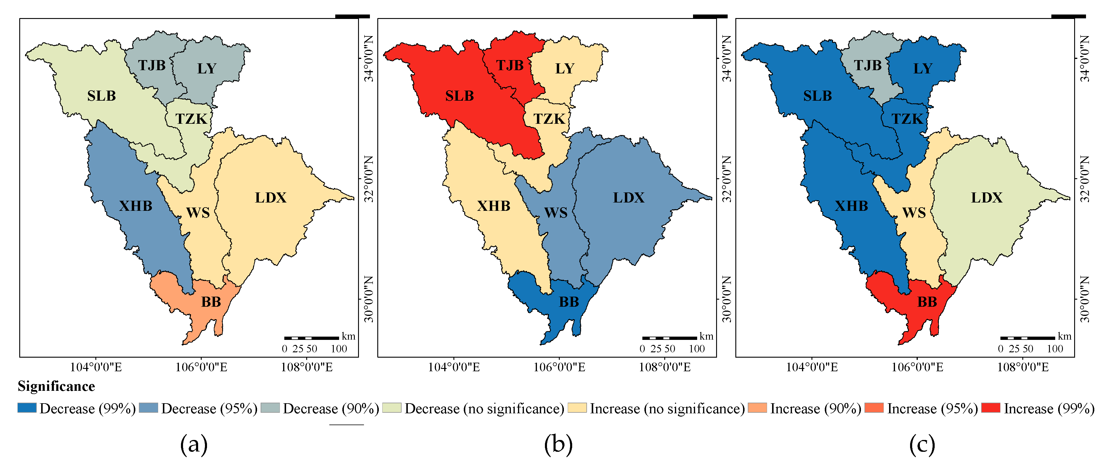
4.1. Temporal-Spatial Alterations of the Hydrometeorological Variables

The nonparametric Mann–Kendall test and Theil–Sen estimator were used to examine the significance of the trends in annual P, E₀, and R across the entire JRW, the composited basin MRW, and the eight sub-basins. The result of trend analyses was summarized and displayed in

Table 1. Mann–Kendall test and Sen’s slope estimator analysis results for discharge.

Region	Period of R	Z Statistics			Slope (β)			Trend
		P	E0	R	P	E0	R	P	E0	R
TJB	1960–2009	−1.446	3.268	−1.33	−0.993	1.339	−0.676	↓ *	↑ ***	↓ *
LY	1960–2000	−1.458	0.972	−2.527	−1.372	0.329	−3.272	↓ *	↑ ns	↓ ***
SLB	1960–2000	−0.51	3.827	−2.819	−0.313	1.11	−3.67	↓ ns	↑ ***	↓ ***
TZK	1960–2000	−0.753	0.049	−2.662	−0.743	0.022	−10.979	↓ ns	↑ ns	↓ ***
XHB	1954–2015	−1.98	0.194	−3.098	−1.772	0.077	−2.512	↓ **	↑ ns	↓ ***
WS	1960–2000	0.109	−2.284	0.461	0.218	−0.71	1.353	↑ ns	↓ **	↑ ns
LDX	1954–2015	1.106	−2.017	−0.753	1.573	−0.597	−0.891	↑ ns	↓ **	↓ ns
BB	1954–2015	1.628	−2.77	3.086	1.908	−1.101	5.951	↑ *	↓ ***	↑ ***
MRW	1954–2015	−0.826	1.859	−1.664	−0.548	0.468	−1.133	↓ ns	↑ *	↓ *
JRW	1954–2015	−0.194	0.207	−2.831	−0.172	0.066	−1.868	↓ ns	↑ ns	↓ ***

Notes: ↑, ↓ indicates an increasing (decreasing) trend; *** means p < 0.01; ** means p < 0.05; * means p < 0.1; ^ns means no significance. Study period of meteorological variables were 1954–2015.

and Figure 2. For the entire JRW, a non-significant decreased P and increased E₀ and significant decreased trend of R were detected with the slopes of −1.72 mm/10a, 0.66 mm/10a, and −18.68 mm/10a, respectively. On a sub-basin scale, trends over the whole time-domain for different regions showed evident spatial patterns. As shown in Figure 2a, the annual P decreased for sub-basins of TJB, LY, SLB, TZK, and SHB, which were located in the northwest part with mountainous terrain, but increased in sub-basins of WS, LDX, and BB, which were located downstream with a plain topography. In contrast, E₀ showed the exact opposite spatial distribution to that of P (Figure 2b): uptrends for the upstream mountainous regions and downtrends for the downstream plain areas. Critically, the spatial pattern of the significance magnitude of varying tendency shown in Figure 2b was in accordance with that of the terrain distribution shown in Figure 1c, which could potentially correlate the climate change to the known elevation transitional feature of the Eeastern Tibet Plateau. As a result of the combined effects of P and E₀, R showed decreasing trends in the northwest sub-basins and increasing trends for the southeast regions that were located downstream and had a lower elevation and more intensive human activities (Figure 2c).

Overall, the opposite tendency of P and E₀ was detected in each sub-region. Therein, decreasing P and increasing E₀ occurred in sub-regions which contain part of the Eastern Tibetan Plateau featured in high-altitude mountains (TJB, LY, SLB, TZK, and XHB). In the middle-low and eastern reaches with a hilly and parallel ridge-valley at a lower elevation, reverse trends of P and E₀ were found (WS, LDX, and BB). This regularity also applied to R, except for LDX, which exhibited no significantly decreased trend, possibly owing to its practical water configuration and management. Additionally, the trend of R in most regions coincided with P or −E₀, indicating the inextricable link between R and climatic factors. Moreover, although the lower reaches section displayed reverse trends, changes of hydrometeorological variables in MRW and JRW were fairly consistent with the upper reaches, which implied the non-negligible impact of the plateau and mountainous areas in the upstream region, as well as the effect from the river network connection between these sub-basins.

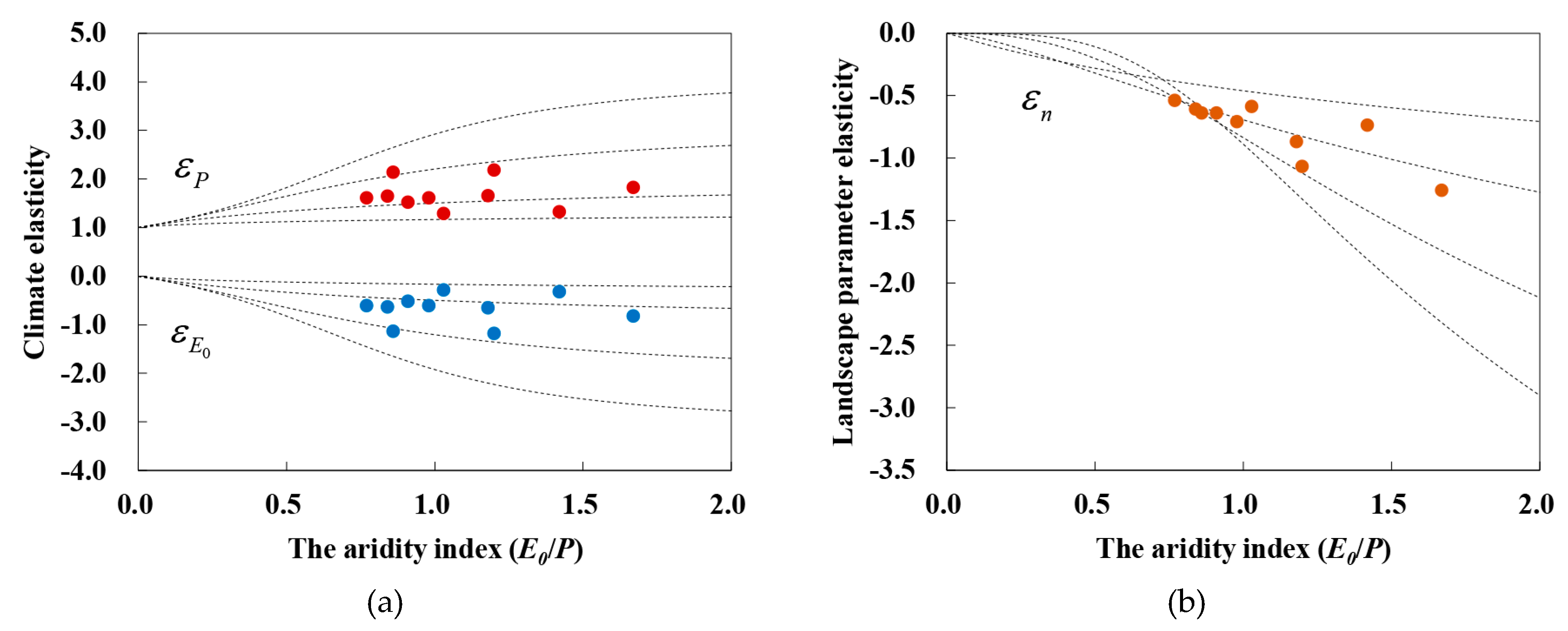
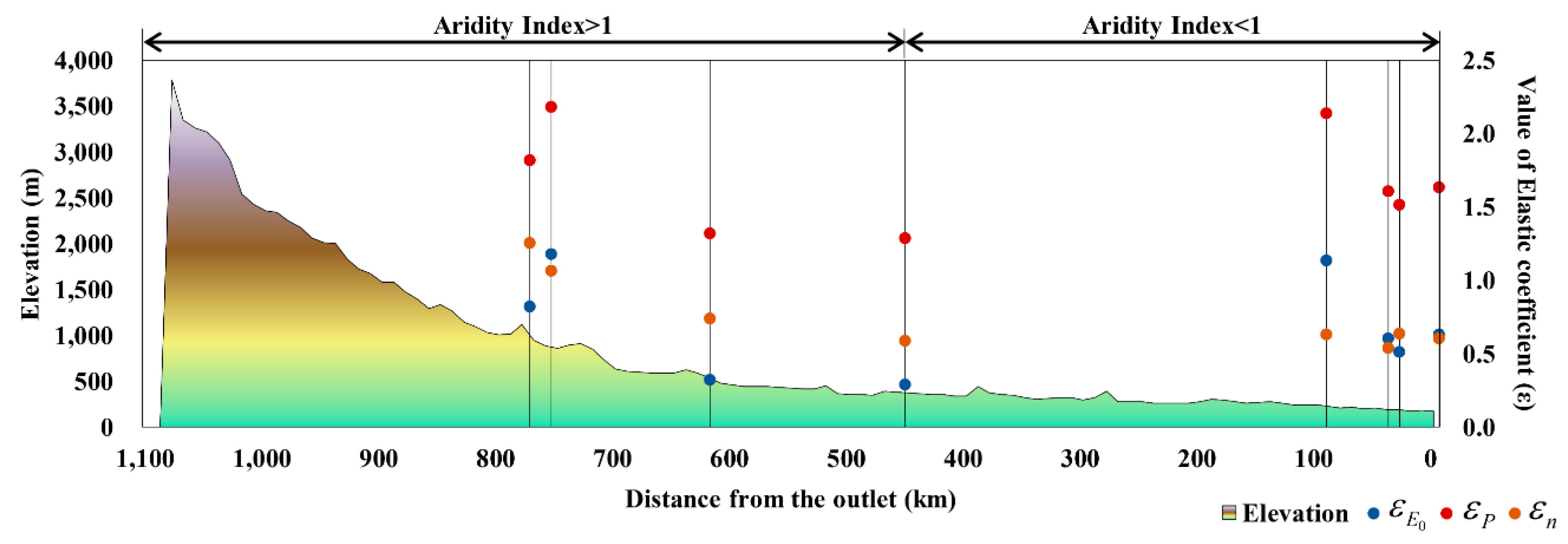
4.2. Sensitivity of Streamflow Alterations to P, E₀, and n

The elastic coefficient represents the influence of one driving factor by unit change, which is also known as the runoff sensitivity. Figure 3 exhibits the positive, negative, and negative values of ${\epsilon }_P$, ${\epsilon }_{E_0}$, and ${\epsilon }_n$. The dotted line in Figure 3 shows the theoretical relationship between the elasticity of runoff and the aridity index (E₀/P). Given ${\epsilon }_P$ + ${\epsilon }_{E_0}$ = 1 [61], the two coefficients always have a contrary sign, where a larger number of ${\epsilon }_P$ means a larger negative value of ${\epsilon }_{E_0}$, indicating the consistent sensitivity of streamflow to P and E₀. With the same parameter n, the absolute value of the elastic coefficient increased with the aridity index. However, when the aridity index rose to a certain extent, ${\epsilon }_P$ and ${\epsilon }_{E_0}$ increased more slowly, while ${\epsilon }_n$ changed more sharply in drier conditions. This implied that runoff was more susceptible in relatively arid areas and the non-climatic impact became more vital under the drier condition along with the limited climatic impact.

Spatial variations of the aridity index and elastic coefficients over the eight sub-sections, MRW, and JRW are displayed in Figure 4 and

Table 2. Hydrometeorological characteristics of sub-regions in the Jialing River Basin.

Region	Period	Drainage Area (km2)	Annual E0 (mm)	Annual P (mm)	Annual R (mm)	E0/P	R/P	n	Elasticity of Runoff
									${\mathit{\epsilon }}_{\mathit{P}}$	${\mathit{\epsilon }}_{{\mathit{E}}_0}$	${\mathit{\epsilon }}_{\mathit{n}}$
TJB	1960–2009	9535	935.33	559.42	166.55	1.67	0.3	1.21	1.82	−0.82	−1.26
LY	1960–2000	9671	901.47	753.39	197.33	1.2	0.26	1.79	2.18	−1.18	−1.07
SLB	1960–2000	29,273	873.49	615.14	354.55	1.42	0.58	0.68	1.32	−0.32	−0.74
TZK	1960–2000	12,610	914.99	892.22	562.68	1.03	0.63	0.69	1.29	−0.29	−0.59
XHB	1954–2015	28,901	869.07	957.09	482.94	0.91	0.5	1.06	1.52	−0.52	−0.64
WS	1960–2000	18,625	882.56	1026.9	346.24	0.86	0.34	2.1	2.14	−1.14	−0.64
LDX	1954–2015	38,064	894.44	1159.14	567.5	0.77	0.49	1.3	1.61	−0.61	−0.54
BB	1954–2015	10,057	873.09	1037.54	483.87	0.84	0.47	1.29	1.64	−0.64	−0.61
MRW	1954–2015	79,714	901.63	766.79	313.76	1.18	0.41	1.15	1.65	−0.65	−0.87
JRW	1954–2015	156,736	892.53	912.8	415.78	0.98	0.46	1.16	1.61	−0.61	−0.71

. The aridity index exhibited a marked downward trend from the upstream to the downstream of the JRW, which was separated into the semi-humid region and humid region by the line of Aridity Index = 1. This changing pattern of the aridity index in space agreed well with that of the hydrometeorological variables presented in Section 4.1. Although the elasticity and aridity index did not show an explicit and clear functional relationship across JRW, greater values and spatial heterogeneity of elastic coefficients were observed in the semi-humid area in the upper reaches, indicating that streamflow in this area was more sensitive and susceptible to climate and catchment landscape change. Significantly, ${\epsilon }_n$ in the upper reaches was higher than other regions, with a monotonic decreasing trend from −1.26 to −0.59 along with the variation of drought conditions. According to the Mezentsev–Choudhury–Yang function, the aridity index and n were the two main factors influencing the elastic coefficients (Figure 3). Thus, as the drought condition across the watershed exhibited a linear change across the whole watershed, the most rational cause for the elasticities’ irregular diversity was the dissimilarity of n values, which ranged from 0.69–2.1, without showing an obvious spatial regularity (Table 2).

The importance of the spatial heterogeneity of land surface property n, presented in Table 2, could also be interpreted by the mean annual water-energy balance function [26], in which regions could be classified as water-limited (arid region without enough P) or energy-limited (humid region without enough E₀) regions. On the ground of this hypothesis, larger n commonly corresponded to smaller runoff coefficients R/P due to the limitation supply of water (P) or energy (E₀). In comparison, for a watershed in which water and energy were in a balanced state, the watershed would yield more runoff and be featured with a small n value [31]. Underpinned by this water-energy balance theory, WS presented the largest n value and the smallest runoff coefficient of 0.34, which was mainly due to the limited E₀ in the humid region. In the semi-humid area, limited precipitation led to the largest n in LY in the upper reaches. With the balance of actual evapotranspiration and precipitation, SLB and TZK presented the smallest n values of 0.68 and 0.69 as the runoff coefficient increased to 0.58 and 0.63, respectively.

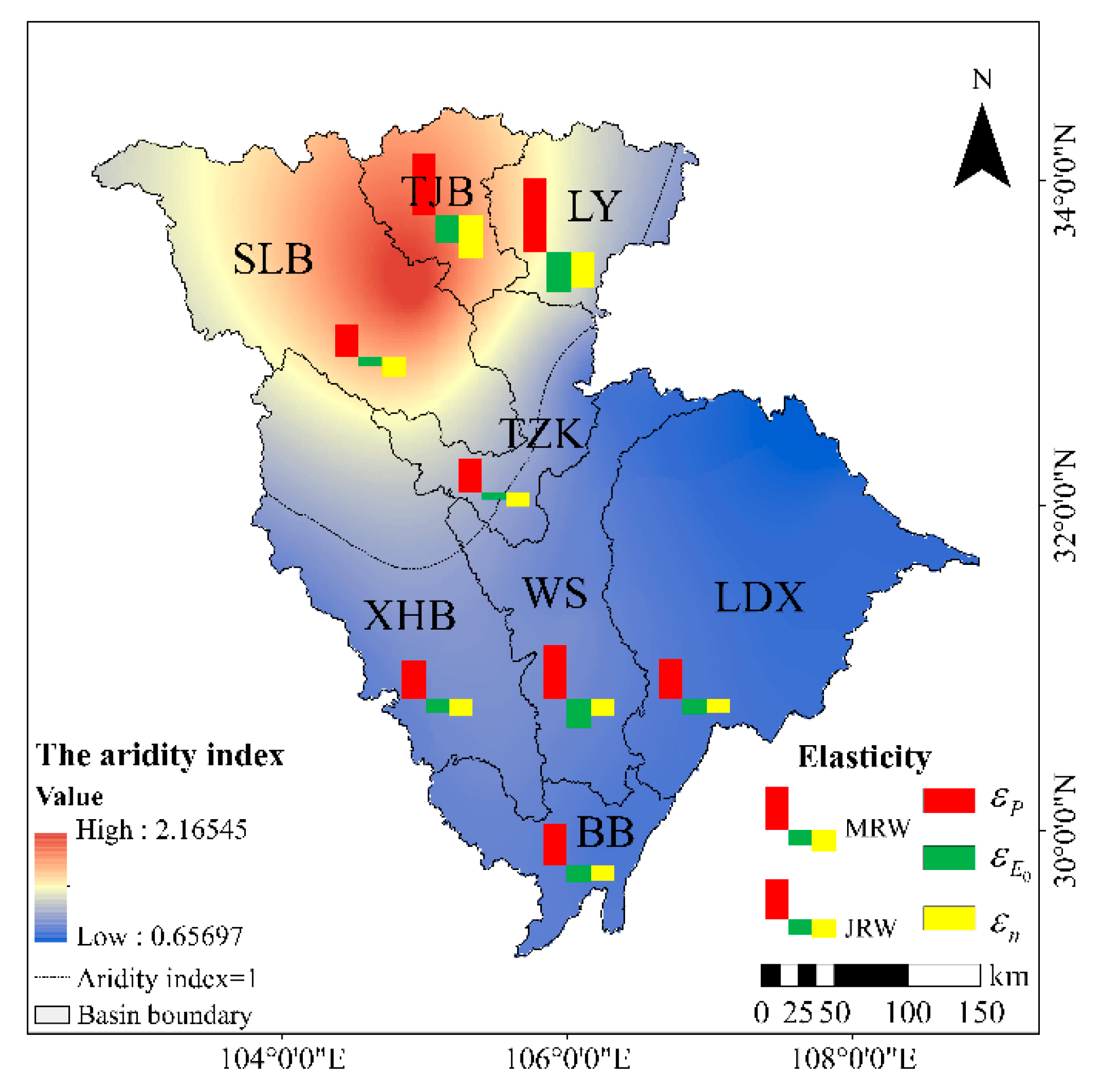
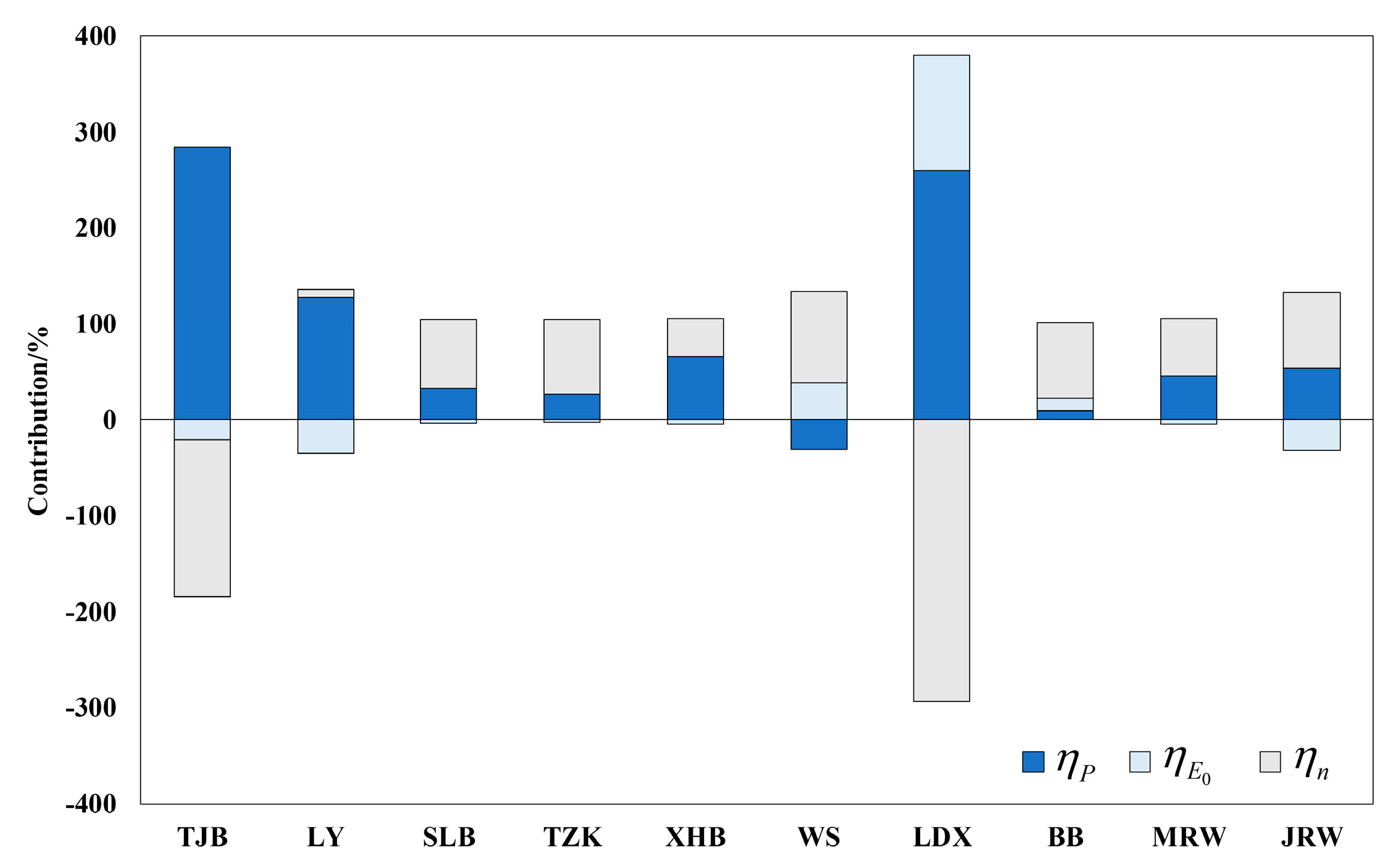
4.3. Spatial-Temporal Variations of Contributions of Driving factors to Streamflow Alteration

The Pettitt test was implemented to determine the abrupt change points for annual precipitation, potential evapotranspiration, and the runoff depth series, which were further used for contribution analysis. The results showed that most regions had breakpoints in annual precipitation at the 5% significance level in 1990, and the abrupt change of potential evapotranspiration approximately appeared in 1979 for most sub-regions. Streamflow records indicated a change point in approximately 1993 due to a lag in the precipitation change in 1990. The results suggested that the hydrometeorological condition was stable before 1979 and the stage could be regarded as a prior impacted period. Therefore, to drive the attribution analysis, the time series was separated into two sub-periods (prior-impacted period-0 and post-impacted period-1) for 1979 using Equation (19a–d). The result is displayed in

Table 3. Runoff variation and attribution analysis for the Jialing River Basin.

Region	Period	R	P	E0	ΔR	ΔP	ΔE0	$\mathbf{\Delta }{\mathit{R}}_{\mathit{P}}$	$\mathbf{\Delta }{\mathit{R}}_{{\mathit{E}}_0}$	$\mathbf{\Delta }{\mathit{R}}_{\mathit{C}}$	${\mathit{\mu }}_{\mathit{C}\mathit{L}\mathit{I}\mathit{M}\mathit{A}\mathit{T}\mathit{E}}$	${\mathit{\mu }}_{\mathit{C}}$
		(mm)	(mm)	(mm)	(mm)	(mm)	(mm)	(mm)	(mm)	(mm)	%	%
TJB	1960–1979	169.96	576.67	939.45	—	—	—	—	—	—	—	—
	1980–2009	164.28	546.96	931.64	−5.68	−29.71	−7.81	−16.14	1.19	9.3	263.85	−163.85
LY	1960–1979	211.42	782.72	919.85	—	—	—	—	—	—	—	—
	1980–2000	183.92	722.34	883.72	−27.51	−60.38	−36.13	−35.21	9.62	−2.31	91.61	8.39
SLB	1960–1979	378.91	624.58	880.02	—	—	—	—	—	—	—	—
	1980–2000	331.35	604.99	866.11	−47.56	−19.58	−13.91	−15.31	1.73	−34.43	27.6	72.4
TZK	1960–1979	697.21	929.4	940.32	—	—	—	—	—	—	—	—
	1980–2000	434.56	850.89	889.94	−262.65	−78.52	−50.38	−68.68	6.2	−207.72	20.91	79.09
XHB	1954–1979	519.8	988.03	875.7	—	—	—	—	—	—	—	—
	1980–2015	456.31	934.75	864.27	−63.48	−53.28	−11.43	−41.43	3.24	−25.92	59.16	40.84
WS	1960–1979	309.06	1040.59	913.56	—	—	—	—	—	—	—	—
	1980–2000	381.65	1008.59	852.6	72.59	−32.01	−60.96	−22.54	28.28	68.61	5.48	94.52
LDX	1954–1979	559.68	1133.05	921.36	—	—	—	—	—	—	—	—
	1980–2015	573.14	1177.97	875	13.46	44.92	−46.37	34.97	16.23	−39.63	394.29	−294.29
BB	1964–1979	394.62	1042.61	905.98	—	—	—	—	—	—	—	—
	1980–2015	548.32	1063.42	858.21	153.7	20.81	−47.77	15.12	19.15	120.34	21.7	78.3
MRW	1954–1979	340.57	784.21	906.94	—	—	—	—	—	—	—	—
	1980–2015	294.39	754.22	897.8	−46.17	−29.99	−9.13	−20.84	2.06	−27.88	39.61	60.39
JRW	1954–1979	426.21	920.47	904.63	—	—	—	—	—	—	—	—
	1980–2015	408.24	907.26	883.79	−17.97	−13.21	−20.83	−9.7	5.75	−14.16	21.19	78.81

and Figure 5. For the entire JRW, contribution of climatic and non-climatic factors were 21.19% and 78.81%, respectively. The larger impact of non-climatic factors was confirmed by previous studies conducted in JRW [34,39], and the main reasons for this phenomenon relate to the intensive anthropogenic disturbances [46], and the fact that the opposite effects of P and E₀ may cancel each other and lead to the small overall climate effect (Figure 5). In addition, the undetectable contribution attributed to non-climatic influence was another reason that will be proposed in the Discussion section. Furthermore, the contribution of each factor varied spatially across the JRW. As shown in Figure 5, climatic effects were high in TJB, LY, XHB, and LDX, but were smaller in SLB, TZK, WS, and BB.

Temporal changes of fractional contributions were further analyzed, before which, the year 1990 was chosen as the second point according to the result of the Pettitt test, which partitioned the whole time period into sub-periods, namely, prior-impacted period-0 (1954/1960–1979) to post-impacted period-2 (1980–1993/2000) and period-0 to post-impacted period-3 (1994–2009/2015). To meet the requirement that time series should be at least 10 years long in statistical analyses, only TJB, XHB, LDX, BB, MRW, and JRW were involved and the ratios of ${\eta }_{CLIMATE}$ and ${\eta }_C$ are shown in

Table 4. Contribution variation in two post-impacted stages.

Region	${\mathit{\eta }}_{\mathit{C}\mathit{L}\mathit{I}\mathit{M}\mathit{A}\mathit{T}\mathit{E}}:{\mathit{\eta }}_{\mathit{C}}$ (Post-Impact Period-2)	${\mathit{\eta }}_{\mathit{C}\mathit{L}\mathit{I}\mathit{M}\mathit{A}\mathit{T}\mathit{E}}:{\mathit{\eta }}_{\mathit{C}}$ (Post-Impact Period-3)	Initial Master Factor	Change of Master Factor
TJB	1:2.04	5.18:1	Catchment properties	↓
XHB	1.79:−1	1.03:1	Climate	↓
LDX	1.48:1	−1:1.79	Climate	↓
BB	1:12.48	1: 5.00	Catchment properties	↓
MRW	−1:4.50	1:2.01	Catchment properties	↓
JRW	1:4.01	1:3.77	Catchment properties	↓

Note: ↓ indicates a decreasing trend of contributing rates.

. For the entire JRW, the contribution rates of climate variables (P, E₀) and landscape properties were approximately 20% and 80%, respectively, for both post-impacted periods. Given that the changes in catchment characteristics were mainly caused by extensive transformation in land use and land cover exerted by severe anthropic activities, human activities should be specifically addressed in watershed management. On a sub-basin scale, the fractional contributions exhibited different tendencies. For sub-basins in upstream regions, such as TJB, the land surface contribution, which was the dominant controlling factor, declined from post-impacted period-2 to post-impacted period-3 after 1993. Comparably, contributions of climatic factors in the downstream tributaries (XHB, LDX), where were controlled by climate elements, descended. Moreover, the contribution variation of the composited basin MRW, which assembles trunk stream sub-basins, was consistent with the upstream sub-basins (TJB), suggesting the vital roles of the plateau and mountainous features region in controlling the meteorological and hydrological conditions. Owing to the river connections between MRW and BB, the contribution trend of sub-basin BB was in accordance with that of the main truck regions. Overall, despite a constant contribution rate all-over the whole JRW, fractional contribution tendencies presented spatial heterogeneity. Remarkably, we found that the contribution weights of master factors were seen to reduce for most sub- and composited-basins (Table 4), indicating that the impacts of these two factors were getting more similar and intricate, and that the contribution partition investigation would become more difficult and complicated in the future.

5. Discussion

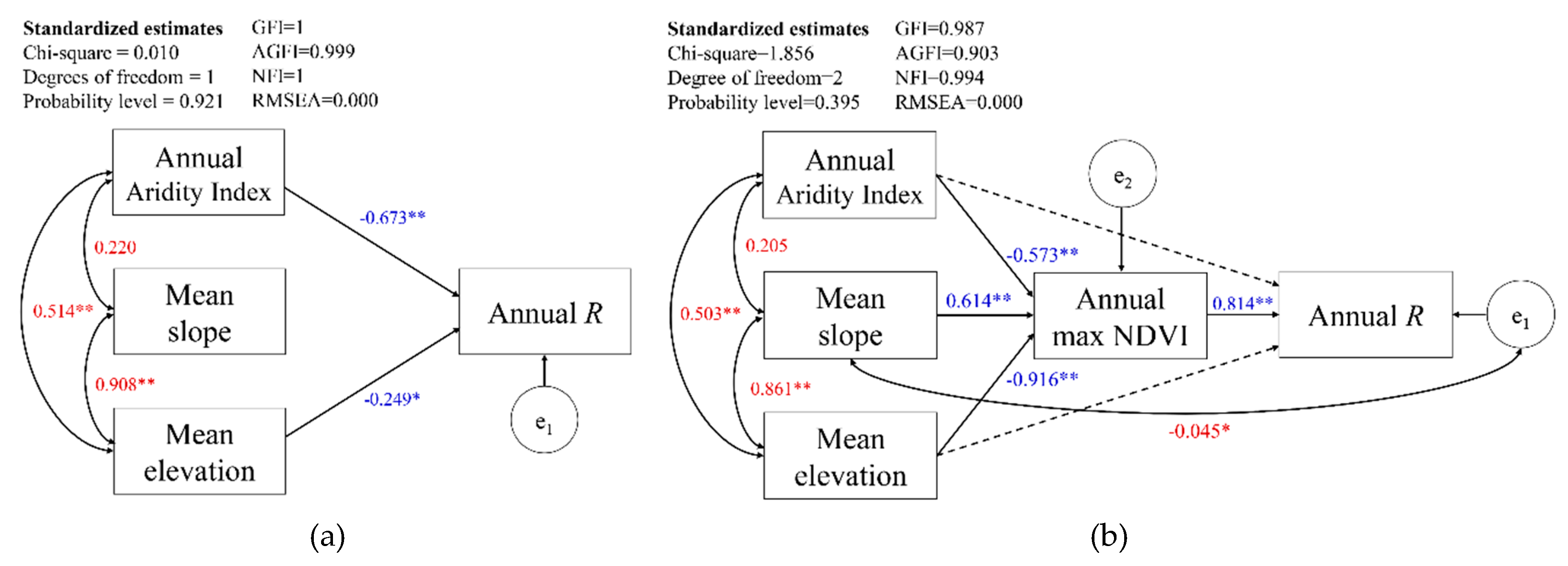
5.1. The Possible Reason for the Temporal-Spatial Heterogeneities

The results of this study presented the spatial and temporal heterogeneity of the hydrological and meteorological variables, the sensitivity of streamflow, and fractional contributions. For spatial heterogeneity over a large watershed, the internal discrepancies of the geographical environment were the main reason of the spatial difference in both climatic and hydrologic properties. The topographic properties, which was not changing with time, mainly include drainage area, average elevation, and catchment slope usually have significant spatial differences. Catchment elevation and its difference usually affects soil properties, basin landforms, and hydrologic processes, thus, elevation was regarded as the original factor of the spatial heterogeneity of streamflow change, which was accompanied by drainage area, climate conditions, and flood confluence processes. Catchment slope also played an important role in effecting the hydrologic process and has been confirmed by previous studies [39], demonstrating a significant logarithmic relationship between the catchment slope and n in China. The potential connection between catchment slope and runoff yield was defined as the water holding capacity, which was higher with a smaller slope and resulted in higher E [39]. Theoretically, parameter n has a positive effect on E and negative effect on R. Moreover, n determined the accuracy of the simulated actual evapotranspiration, and further affected the calculation of sensitivity and attribution. Hence, the distribution of n would help to further understand the runoff generation mechanism. For the JRW, under the same meteorological conditions of P and E₀, a lower R was yielded in WS (n = 2.1) and LY (n = 1.79), while a higher R was obtained in SLB (n = 0.68) and TZK (n = 0.69), during the study period. Sensitivity of runoff also bored relation to topographic properties. Namely, for upstream regions with a higher elevation and more complex topography, runoff tended to display a greater sensitivity and spatial heterogeneity. In general, the elasticity of runoff to parameter n declined with elevation from the upstream to downstream sub-basins (Figure 6).

The variation of climatic variables and landscape conditions could jointly explain the phenomena of temporal changes of hydrological features and contribution rates. Various studies have been carried out worldwide to determine the background of global warming and continuous land cover change. Alteration of contribution rates has also been emphasized [62]. Compared with previous studies, we analyzed the contribution alteration in both time and space domains in the JRW. In this study, the contributions of six districts (Table 4) in two post-impacted periods were calculated by the Budyko function. Collectively, our study demonstrated the predominant effect of non-climatic factors on runoff in the JRW for the whole impacted period, yet with different contribution modes and variations in sub-basins. Critically, the temporal trends of fractional contributions within sub- and composited basins TJB, BB, and MRW, which were independent and connected by a river network, displayed a consistent tendency (Table 4), indicating the increasingly vital role of climatic factors in streamflow generation and propagation. Nevertheless, the different performances of contribution rates between sub-basins and the entire JRW still called for more explanations on the spatiotemporal heterogeneity of hydrological processes and the internal mechanism of hydrological responses.

5.2. The Synergistic Effects of the Two Driver Factors on Contribution Analyses

The analyses of driving factors’ attribution indicated the synergetic impacts of climate and catchment characteristics on hydrological processes, which were distinctly exhibited in the JRW, i.e., the characteristics of meteorological and topographic elements were affinitive with each other. In detail, P and E₀ of sub-basins varied with significant spatial regulation, and the aridity index of the JRW also decreased monotonously from the upper stream to lower reaches. When calculating fractional contributions based on the Budyko complementary method, the formulation attributed the climate impact to P and E₀, and watershed characteristics to parameter n, respectively, and this hypothesis was interpreted in Equation (10). It can be derived from this equation that the potential residuals caused by meteorological factors would be subsumed into the contribution of catchment characteristics. As a result, in the current framework, catchment properties, known as landform and landscape characteristics, interacted with climatic variables and led to an overestimation of the distinguishing contributions.

As an example, vegetation is an important component in hydrological processes and could be identified as the connection of climate and land surface elements. Though a low correlation of vegetation and streamflow has been proposed in many studies [37,39], the interaction between climatic factors (P, E₀) and topographies elements owing to vegetation could not be ignored [63,64]. In the JRW, the forest cover rate increased from 11.62% to 30.06% during 1973–2013, according to the records of the Nation Forest Resources Inventory (http://www.forestry.gov.cn/gjslzyqc.html). As the impact of vegetation was attributed to non-climatic factors in the Budyko framework, it is unequivocal that changes of vegetation owing to climate change were misclassified. Thus, streamflow alteration caused by climatic factors, which was indirectly reflected by vegetation, would be wrongly attributed to land surface factors. In other words, the contribution of climate was underestimated owing to the synergistic reaction of climatic and non-climatic factors and the framework of the Budyko function.

To verify the above hypothesis, qualitative analysis of the potential interaction between climatic factors (P, E₀), topographic elements (basin mean slope, basin mean elevation), and landform factors (NDVI, Normalized Difference Vegetation Index) was performed by the structural equation model (SEM) using Amos 24, the theory of which was presented in detail in Grace [65] and Malaeb et al. [66]. Two scenarios, without and with vegetation, were set up to detect the relationship and connection among these variables (Figure 7). Note that the NDVI time series was from 2000 to 2015 (MODND1M; http://www.gscloud.cn/), and hydrometeorological generations in SLB, XHB, LDX, and BB were included in the calculation to ensure the independence of terrain factors. Finally, 57 samples with logarithm transformation and standardization were available. In the estimation, we employed the maximum likelihood estimation (MLE) to compute the coefficients and selected significant paths to modify the model. With the model path map displayed in Figure 7, the model fitted well with acceptable ranges of common fit statistics: Probability level > 0.05, GFI > 0.90, AGFI > 0.90, NFI > 0.90, RMSEA < 0.05. The correlation coefficient stood for the interaction among influencing factors, while the standardized regression weight represented the direct and indirect impact of multi-variables on streamflow. Figure 7a exhibits the direct and significant (p < 0.05) relationship between R and the two driving factors. Simultaneously, the significant correlation between the topographic factor and climatic condition indicated the interaction of these two factors. In Figure 7b, by adding the influence of the vegetation, direct influences from both climatic and topographic factors became much smaller and the corresponding paths were deleted by the algorithm of the model (dotted line in Figure 7b) and, in consequence, all the exogenous variables firstly affected NDVI (with significant level of p < 0.01) and further acted on runoff through vegetation. In this manner, the indirect effect originally exerted by climatic factors would be wrongly attributed to the NDVI, which was regarded as the land surface factor. Thus, the total effect of climatic factors was reduced in two ways, i.e., the decreased direct effect between climatic factors and R, and the misclassification of the indirect effect exerted by climate. In summary, the influencing factors were inter-related with each other, confirming the synergistic effect of influencing factors on river runoff. More importantly, the important function the vegetation played, as a transitional form between climatic and topographic factors and streamflow, would underestimate the function of climate elements while overestimating that of the topographic elements. These findings provided evidence that the synergistic effect of driving factors would be prone to cause deviation and complicate contribution analyses by adding a new dimension to the issue.

Overall, the climatic and non-climatic factors were proved to act on streamflow in a synergistic way, which is a challenge in attribution analysis in the future. With the transitional role of vegetation, the attribution analyses would result in an underestimation of the climate effect. Hence, more explorations on the improvement of the attribution method are expected with the background of climate change, intense landcover transformation, and severe anthropic interference.

6. Conclusions

The objective of this study was to quantify the relative impact of climate variability and land surface disturbance on the spatial-temporal variation of the JRW, which was divided into eight sub-basins by eight hydrologic stations. The JRW is geographically located in the first terrain gradient band in China, which is the transition zone of Qinghai-Tibet Plateau and Sichuan Basin and, thus, shows distinctive climatic and topographic features from the upstream and downstream sub-basins. Statistical methods, the Mann–Kendall test, Sen’s slope estimator, and the Pettitt test, were used for tendency and abrupt change detection, and the elastic coefficient method and a complementary method based on the Mezentsev–Choudhury–Yang function were adopted to analyze the sensitivity and fractional contribution of streamflow to the two driving factors on both temporal and spatial scales. The main findings are as follows:

The tendencies of meteorological and hydrological elements (P, E₀, and R) showed spatial regularities across the JRW. In detail, R decreased significantly for the entire region, consistent with the upper reaches, which were characterized by a semi-humid climate and mountainous terrain, indicating the notable effects of mountainous topography on the whole watershed, as well as the effect of river network connections between these sub-basins. Comparably, R increased in the lower reaches, which were characterized by a humid climate and plain topography. Temporal changes of P and E₀ in sub-basins showed similar schemes.

Runoff generation was more sensitive and susceptible to climate and catchment landscape in semi-humid areas than that of humid regions according to the aridity condition. Moreover, the mean annual water-energy balance function fairly explained the importance of spatial heterogeneity of the land surface property n to runoff sensitivity.

With the breaking point in 1979, non-climatic factors accounted for 80% fractional contribution of the total streamflow alteration in the JRW, while exhibiting spatial heterogeneity in sub-basins. By adding a breaking point at 1990, tendencies of contribution rates were calculated for basins on different spatial scales: the JRW showed a nearly unchangeable contribution rate, and a changeable tendencies interior of the watershed. In sub- and composited basins, the impact of the primary influencing factor on sub-basins exhibited a decreasing trend, manifesting more similar and intricate roles of these two driving factors and thus a more complicated phenomenon in attribution analyses.

References

1. Milly, P.C.; Dunne, K.A.; Vecchia, A.V. Global pattern of trends in streamflow and water availability in a changing climate. Nature 2005, 438, 347–350. [Google Scholar] [CrossRef] [PubMed]
2. Cuo, L.; Beyene, T.K.; Voisin, N.; Su, F.; Lettenmaier, D.P.; Alberti, M.; Richey, J.E. Effects of mid-twenty-first century climate and land cover change on the hydrology of the Puget Sound Basin, washington. Hydrol. Process. 2011, 25, 1729–1753. [Google Scholar] [CrossRef]
3. van Roosmalen, L.; Sonnenborg, T.O.; Jensen, K.H. Impact of climate and land use change on the hydrology of a large-scale agricultural catchment. Water Resour. Res. 2009, 45. [Google Scholar] [CrossRef] [Green Version]
4. Sterling, S.M.; Ducharne, A.; Polcher, J. The impact of global land-cover change on the terrestrial water cycle. Nat. Clim. Chang. 2012, 3, 385–390. [Google Scholar] [CrossRef]
5. Carvalho-Santos, C.; Nunes, J.P.; Monteiro, A.T.; Hein, L.; Honrado, J.P. Assessing the effects of land cover and future climate conditions on the provision of hydrological services in a medium-sized watershed of Portugal. Hydrol. Process. 2016, 30, 720–738. [Google Scholar] [CrossRef]
6. Serpa, D.; Nunes, J.P.; Santos, J.; Sampaio, E.; Jacinto, R.; Veiga, S.; Lima, J.C.; Moreira, M.; Corte-Real, J.; Keizer, J.J.; et al. Impacts of climate and land use changes on the hydrological and erosion processes of two contrasting Mediterranean catchments. Sci. Total Environ. 2015, 538, 64–77. [Google Scholar] [CrossRef] [Green Version]
7. Buendia, C.; Batalla, R.J.; Sabater, S.; Palau, A.; Marcé, R. Runoff trends driven by climate and afforestation in a Pyrenean basin. Land Degrad. Dev. 2016, 27, 823–838. [Google Scholar] [CrossRef]
8. Napoli, M.; Massetti, L.; Orlandini, S. Hydrological response to land use and climate changes in a rural hilly basin in Italy. Catena 2017, 157, 1–11. [Google Scholar] [CrossRef]
9. Wu, J.; Miao, C.; Wang, Y.; Duan, Q.; Zhang, X. Contribution analysis of the long-term changes in seasonal runoff on the loess plateau, china, using eight Budyko-based methods. J. Hydrol. 2017, 545, 263–275. [Google Scholar] [CrossRef]
10. Bronstert, A.; Niehoff, D.; Bürger, G. Effects of climate and land-use change on storm runoff generation: Present knowledge and modelling capabilities. Hydrol. Process. 2002, 16, 509–529. [Google Scholar] [CrossRef]
11. IPCC. Climate Change 2014—Impacts, Adaptation and Vulnerability: Regional Aspects; Cambridge University Press: Cambridge, UK, 2014. [Google Scholar]
12. Ali, S.; Sethy, B.K.; Singh, R.K.; Parandiyal, A.K.; Kumar, A. Quantification of hydrologic response of staggered contour trenching for Horti-pastoral land use system in small ravine watersheds: A paired watershed approach. Land Degrad. Dev. 2017, 28, 1237–1252. [Google Scholar] [CrossRef]
13. King, K.W.; Smiley, P.C.; Baker, B.J.; Fausey, N.R. Validation of paired watersheds for assessing conservation practices in the upper big Walnut Creek Watershed, Ohio. J. Soil Water Conserv. 2008, 63, 380–395. [Google Scholar] [CrossRef]
14. Miller, E.L. Sediment yield and storm flow response to clear-cut harvest and site preparation in the Ouachita mountains. Water Resour. Res. 1984, 20, 471–475. [Google Scholar] [CrossRef]
15. Clausen, J.C.; Jokela, W.E.; Potter, F.I.; Williams, J.W. Paired watershed comparison of tillage effects on runoff, sediment, and pesticide losses. J. Environ. Qual. 1996, 25, 1000–1007. [Google Scholar] [CrossRef]
16. Worqlul, A.W.; Ayana, E.K.; Yen, H.; Jeong, J.; Macalister, C.; Taylor, R.; Gerik, T.J.; Steenhuis, T.S. Evaluating hydrologic responses to soil characteristics using swat model in a paired-watersheds in the upper blue Nile basin. Catena 2018, 163, 332–341. [Google Scholar] [CrossRef]
17. Hayashi, S.; Murakami, S.; Xu, K.Q.; Watanabe, M. Simulation of the reduction of runoff and sediment load resulting from the gain for green program in the Jialingjiang catchment, upper region of the Yangtze river, china. J. Environ. Manag. 2015, 149, 126–137. [Google Scholar] [CrossRef]
18. Marhaento, H.; Booij, M.J.; Rientjes, T.H.M.; Hoekstra, A.Y. Attribution of changes in the water balance of a tropical catchment to land use change using the swat model. Hydrol. Process. 2017, 31, 2029–2040. [Google Scholar] [CrossRef]
19. Dams, J.; Nossent, J.; Senbeta, T.B.; Willems, P.; Batelaan, O. Multi-model approach to assess the impact of climate change on runoff. J. Hydrol. 2015, 529, 1601–1616. [Google Scholar] [CrossRef]
20. Séguis, L.; Cappelaere, B.; Milési, G.; Peugeot, C.; Massuel, S.; Favreau, G. Simulated impacts of climate change and land-clearing on runoff from a small Sahelian catchment. Hydrol. Process. 2004, 18, 3401–3413. [Google Scholar] [CrossRef]
21. Lørup, J.K.; Refsgaard, J.C.; Mazvimavi, D. Assessing the effect of land use change on catchment runoff by combined use of statistical tests and hydrological modelling: Case studies from Zimbabwe. J. Hydrol. 1998, 205, 147–163. [Google Scholar] [CrossRef]
22. Karl, T.R.; Riebsame, W.E. The impact of decadal fluctuations in mean precipitation and temperature on runoff: A sensitivity study over the United States. Clim. Chang. 1989, 15, 423–447. [Google Scholar] [CrossRef]
23. Siriwardena, L.; Finlayson, B.L.; McMahon, T.A. The impact of land use change on catchment hydrology in large catchments: The Comet river, Central Queensland, Australia. J. Hydrol. 2006, 326, 199–214. [Google Scholar] [CrossRef]
24. Webb, A.A.; Kathuria, A. Response of streamflow to afforestation and thinning at red hill, Murray Darling Basin, Australia. J. Hydrol. 2012, 412–413, 133–140. [Google Scholar] [CrossRef]
25. Gao, P.; Li, P.; Zhao, B.; Xu, R.; Zhao, G.; Sun, W.; Mu, X. Use of double mass curves in hydrologic benefit evaluations. Hydrol. Process. 2017, 31, 4639–4646. [Google Scholar] [CrossRef]
26. Budyko, M. Climate and Life; Academic Press: New York, NY, USA, 1974; 508p. [Google Scholar]
27. Fu, B. On the calculation of the evaporation from land surface. Sci. Atmos. Sin. 1981, 5, 23–31. [Google Scholar]
28. Schaake, J.C. From climate to flow. Clim. Chang. US Water Resour. 1990, 177–206. [Google Scholar]
29. Mezentsev, V. More on the calculation of average total evaporation. Meteorol. Gidrol. 1955, 5. [Google Scholar]
30. Choudhury, B. Evaluation of an empirical equation for annual evaporation using field observations and results from a biophysical model. J. Hydrol. 1999, 216, 99–110. [Google Scholar] [CrossRef]
31. Yang, H.; Yang, D.; Lei, Z.; Sun, F. New analytical derivation of the mean annual water-energy balance equation. Water Resour. Res. 2008, 44. [Google Scholar] [CrossRef]
32. Zhang, L.; Dawes, W.R.; Walker, G.R. Response of mean annual evapotranspiration to vegetation changes at catchment scale. Water Resour. Res. 2001, 37, 701–708. [Google Scholar] [CrossRef]
33. Zhou, G.; Wei, X.; Chen, X.; Zhou, P.; Liu, X.; Xiao, Y.; Sun, G.; Scott, D.F.; Zhou, S.; Han, L. Global pattern for the effect of climate and land cover on water yield. Nat. Commun. 2015, 6, 5918. [Google Scholar] [CrossRef] [PubMed]
34. Shen, Q.; Cong, Z.; Lei, H. Evaluating the impact of climate and underlying surface change on runoff within the Budyko framework: A study across 224 catchments in China. J. Hydrol. 2017, 554, 251–262. [Google Scholar] [CrossRef]
35. Luo, K.; Tao, F.; Moiwo, J.P.; Xiao, D. Attribution of hydrological change in Heihe river basin to climate and land use change in the past three decades. Sci. Rep. 2016, 6, 33704. [Google Scholar] [CrossRef] [PubMed]
36. Ahn, K.-H.; Merwade, V. Quantifying the relative impact of climate and human activities on streamflow. J. Hydrol. 2014, 515, 257–266. [Google Scholar] [CrossRef]
37. Li, Z.; Ning, T.; Li, J.; Yang, D. Spatiotemporal variation in the attribution of streamflow changes in a catchment on China’s Loess Plateau. Catena 2017, 158, 1–8. [Google Scholar] [CrossRef]
38. Yang, D.; Sun, F.; Liu, Z.; Cong, Z.; Ni, G.; Lei, Z. Analyzing spatial and temporal variability of annual water-energy balance in nonhumid regions of china using the Budyko hypothesis. Water Resour. Res. 2007, 43. [Google Scholar] [CrossRef]
39. Yang, H.; Qi, J.; Xu, X.; Yang, D.; Lv, H. The regional variation in climate elasticity and climate contribution to runoff across china. J. Hydrol. 2014, 517, 607–616. [Google Scholar] [CrossRef]
40. Ye, X.; Qi, Z.; Jian, L.; Li, X.; Xu, C. Distinguishing the relative impacts of climate change and human activities on variation of streamflow in the Poyang lake catchment, china. J. Hydrol. 2013, 494, 83–95. [Google Scholar] [CrossRef]
41. Ouyang, L.; Liu, S.; Ye, J.; Liu, Z.; Sheng, F.; Wang, R.; Lu, Z. Quantitative assessment of surface runoff and base flow response to multiple factors in Pengchongjian small watershed. Forests 2018, 9, 553. [Google Scholar] [CrossRef]
42. Wang, W.; Zou, S.; Shao, Q.; Xing, W.; Chen, X.; Jiao, X.; Luo, Y.; Yong, B.; Yu, Z. The analytical derivation of multiple elasticities of runoff to climate change and catchment characteristics alteration. J. Hydrol. 2016, 541, 1042–1056. [Google Scholar] [CrossRef]
43. Merz, R.; Blöschl, G.; Parajka, J. Spatio-temporal variability of event runoff coefficients. J. Hydrol. 2006, 331, 591–604. [Google Scholar] [CrossRef]
44. Kuraś, P.K.; Weiler, M.; Alila, Y. The spatiotemporal variability of runoff generation and groundwater dynamics in a snow-dominated catchment. J. Hydrol. 2008, 352, 50–66. [Google Scholar] [CrossRef]
45. Zhao, G.; Mu, X.; Jiao, J.; An, Z.; Klik, A.; Wang, F.; Jiao, F.; Yue, X.; Gao, P.; Sun, W. Evidence and causes of spatiotemporal changes in runoff and sediment yield on the Chinese loess plateau. Land Degrad. Dev. 2017, 28, 579–590. [Google Scholar] [CrossRef]
46. Yan, Y.; Wang, S.; Chen, J. Spatial patterns of scale effect on specific sediment yield in the Yangtze River basin. Geomorphology 2011, 130, 29–39. [Google Scholar] [CrossRef]
47. Chen, J.; Wu, X.; Finlayson, B.L.; Webber, M.; Wei, T.; Li, M.; Chen, Z. Variability and trend in the hydrology of the Yangtze River, china: Annual precipitation and runoff. J. Hydrol. 2014, 513, 403–412. [Google Scholar] [CrossRef]
48. Chen, J.; Finlayson, B.L.; Wei, T.; Sun, Q.; Webber, M.; Li, M.; Chen, Z. Changes in monthly flows in the Yangtze River, china–with special reference to the three gorges dam. J. Hydrol. 2016, 536, 293–301. [Google Scholar] [CrossRef]
49. Kundu, S.; Khare, D.; Mondal, A. Individual and combined impacts of future climate and land use changes on the water balance. Ecol. Eng. 2017, 105, 42–57. [Google Scholar] [CrossRef]
50. Zhou, S.; Yu, B.; Zhang, L.; Huang, Y.; Pan, M.; Wang, G. A new method to partition climate and catchment effect on the mean annual runoff based on the Budyko complementary relationship. Water Resour. Res. 2016, 52, 7163–7177. [Google Scholar] [CrossRef] [Green Version]
51. Mann, H.B. Nonparametric tests against trend. Econom. J. Econom. Soc. 1945, 245–259. [Google Scholar] [CrossRef]
52. Kendall, M. Rank Correlation Measures [m]; Charles Griffin: London, UK.
53. Sen, P.K. Estimates of the regression coefficient based on Kendall’s tau. J. Am. Stat. Assoc. 1968, 63, 1379–1389. [Google Scholar] [CrossRef]
54. Theil, H. A Rank-Invariant Method of Linear and Polynomial Regression Analysis. In Henri Theil’S Contributions to Economics and Econometrics; Springer: Dordrecht, Netherlands, 1992; pp. 345–381. [Google Scholar]
55. Pettitt, A. A non-parametric approach to the change-point problem. Appl. Stat. 1979, 126–135. [Google Scholar] [CrossRef]
56. Eagleson, P.S. Climate, soil, and vegetation: 1. Introduction to water balance dynamics. Water Resour. Res. 1978, 14, 705–712. [Google Scholar] [CrossRef] [Green Version]
57. Liang, W.; Bai, D.; Wang, F.; Fu, B.; Yan, J.; Wang, S.; Yang, Y.; Long, D.; Feng, M. Quantifying the impacts of climate change and ecological restoration on streamflow changes based on a Budyko hydrological model in China’s Loess Plateau. Water Resour. Res. 2015, 51, 6500–6519. [Google Scholar] [CrossRef]
58. Eagleson, P.S. Climate, soil, and vegetation: 7. A derived distribution of annual water yield. Water Resour. Res. 1978, 14, 765–776. [Google Scholar] [CrossRef] [Green Version]
59. Allen, R.G.; Pereira, L.S.; Raes, D.; Smith, M. Crop evapotranspiration-guidelines for computing crop water requirements-FAO irrigation and drainage paper 56. FAO Rome 1998, 300, D05109. [Google Scholar]
60. Donohue, R.J.; Roderick, M.L.; McVicar, T.R. Can dynamic vegetation information improve the accuracy of budyko’s hydrological model? J. Hydrol. 2010, 390, 23–34. [Google Scholar] [CrossRef]
61. Zhou, S.; Yu, B.; Huang, Y.; Wang, G. The complementary relationship and generation of the Budyko functions. Geophys. Res. Lett. 2015, 42, 1781–1790. [Google Scholar] [CrossRef] [Green Version]
62. Tan, X.; Gan, T.Y. Contribution of human and climate change impacts to changes in streamflow of Canada. Sci. Rep. 2015, 5, 17767. [Google Scholar] [CrossRef] [PubMed]
63. Cristea, N.C.; Lundquist, J.D.; Loheide, S.P.; Lowry, C.S.; Moore, C.E. Modelling how vegetation cover affects climate change impacts on streamflow timing and magnitude in the snowmelt-dominated upper Tuolumne basin, Sierra Nevada. Hydrol. Process. 2014, 28, 3896–3918. [Google Scholar] [CrossRef]
64. Peel, M.C.; McMahon, T.A.; Finlayson, B.L.; Watson, F.G.R. Implications of the relationship between catchment vegetation type and the variability of annual runoff. Hydrol. Process. 2002, 16, 2995–3002. [Google Scholar] [CrossRef]
65. Grace, J.B. Structural Equation Modeling and Natural Systems; Cambridge University Press: Cambridge, UK, 2006. [Google Scholar]
66. Malaeb, Z.A.; Summers, J.K.; Pugesek, B.H. Using structural equation modeling to investigate relationships among ecological variables. Environ. Ecol. Stat. 2000, 7, 93–111. [Google Scholar] [CrossRef]
Figure 1. Location and elevation of the JRW and hydrometeorological stations.
Forests 10 00495 g001
Figure 2. Changing trends and significance for (a) P, (b) E0, and (c) R by Z statistics of the Mann–Kendall test.
Forests 10 00495 g002
Figure 3. Relationship between the elasticity ((a) ε P and ε E 0 ; (b) ε n ) of runoff and the aridity index (E0/P). Note: the line represents the elasticity of runoff; a red dot represents ε P , a blue dot represents ε E 0 , and an orange dot represents ε n for the 10 regions.
Forests 10 00495 g003
Figure 4. Spatial distribution of the annual aridity index and elasticity value.
Forests 10 00495 g004
Figure 5. Attribution of R change from prior-impacted period-0 to post-impacted period-1.
Forests 10 00495 g005
Figure 6. Changes of altitude and elastic coefficients in the Jialing River Basin.
Forests 10 00495 g006
Figure 7. The structured equation model ((a) detection of climatic and topographic effects; (b) detection of vegetation’s function). Note: e1 and e2 represent the measurement error of NDVI and R generation, respectively. ** Correlation is signigicant at the 0.001 level (two-tailed). * Correlation is siginificant at the 0.05 level (two-tailed). Numbers in red indicate the correlation coefficient; numbers in blue represent standized regression weights. Dotted lines represent a nonsignificant path of a direct effect.
Forests 10 00495 g007