Factors Influencing the Geographical Distribution of Dendroctonus armandi (Coleoptera: Curculionidae: Scolytidae) in China


Abstract
:1. Introduction
2. Materials and Methods
2.1. Study Area
2.2. Data
2.2.1. Ecogeographical Variables Layers
2.2.2. D. armandi Distribution Data and Geographic Layer
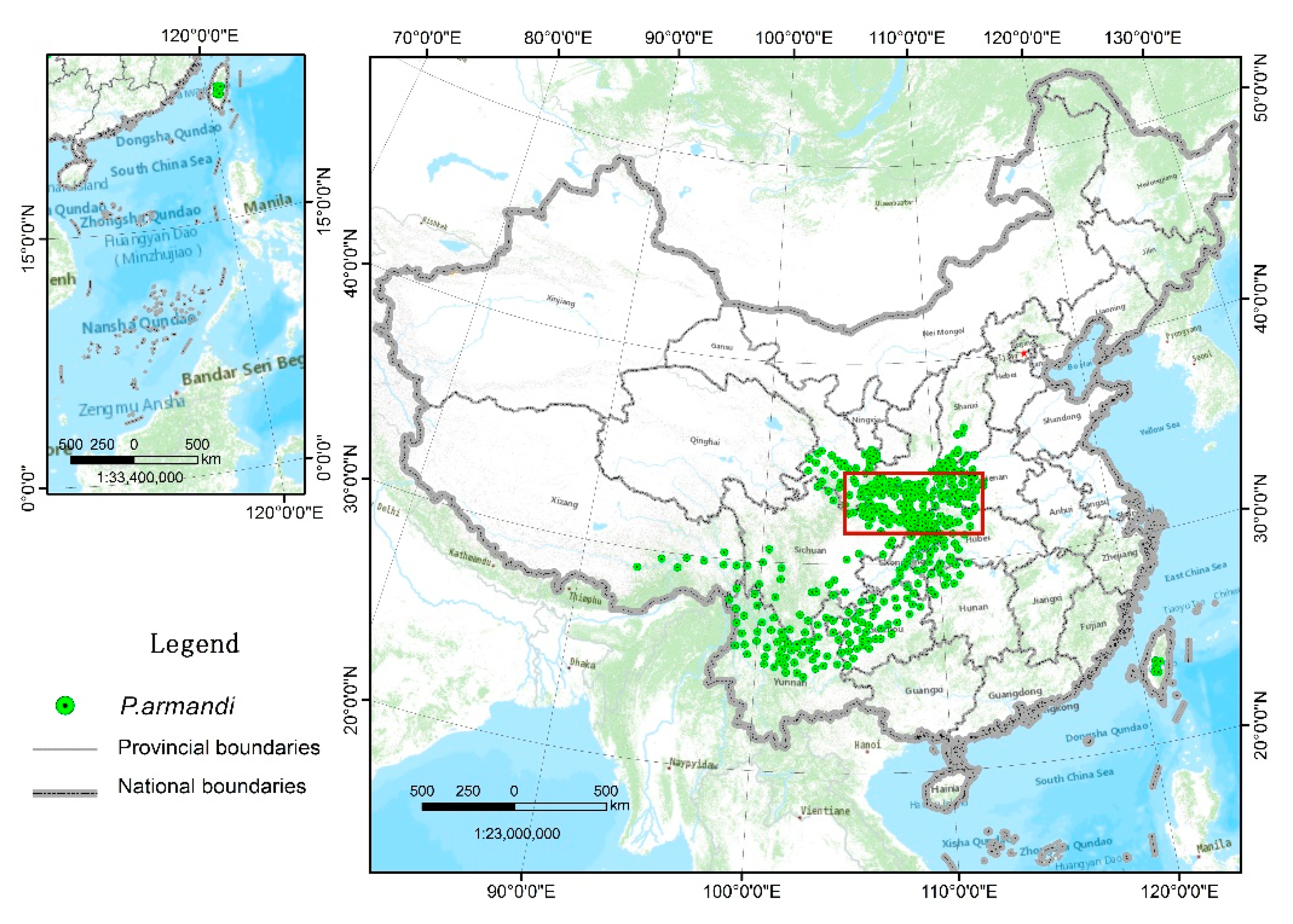
2.2.3. P. armandi Distribution Data
2.3. Bioclimatic Profile of D. armandi
2.4. Current Potential Distribution (SDMs)
2.4.1. Potential Distribution of D. armandi Using BIOCLIM
2.4.2. Potential Distribution of D. armandi Using ENFA
2.4.3. Potential Distribution of D. armandi Using MaxEnt
3. Results
3.1. Bioclimatic Profile of D. armandi
3.2. Variables Selection
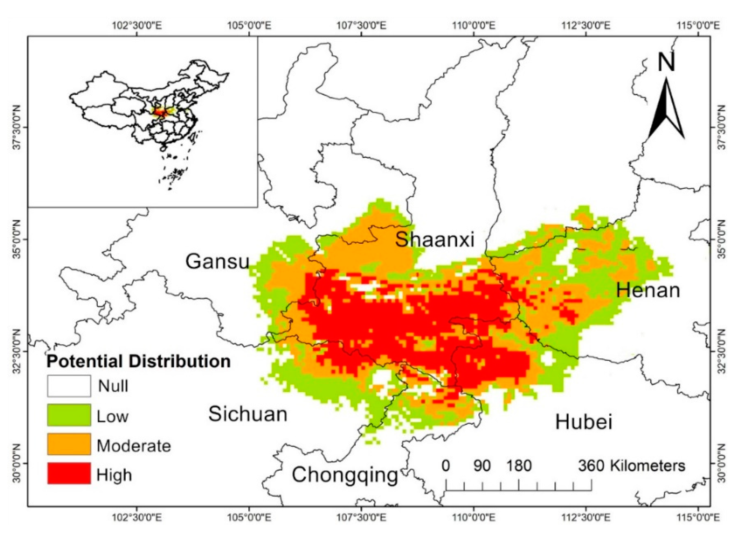
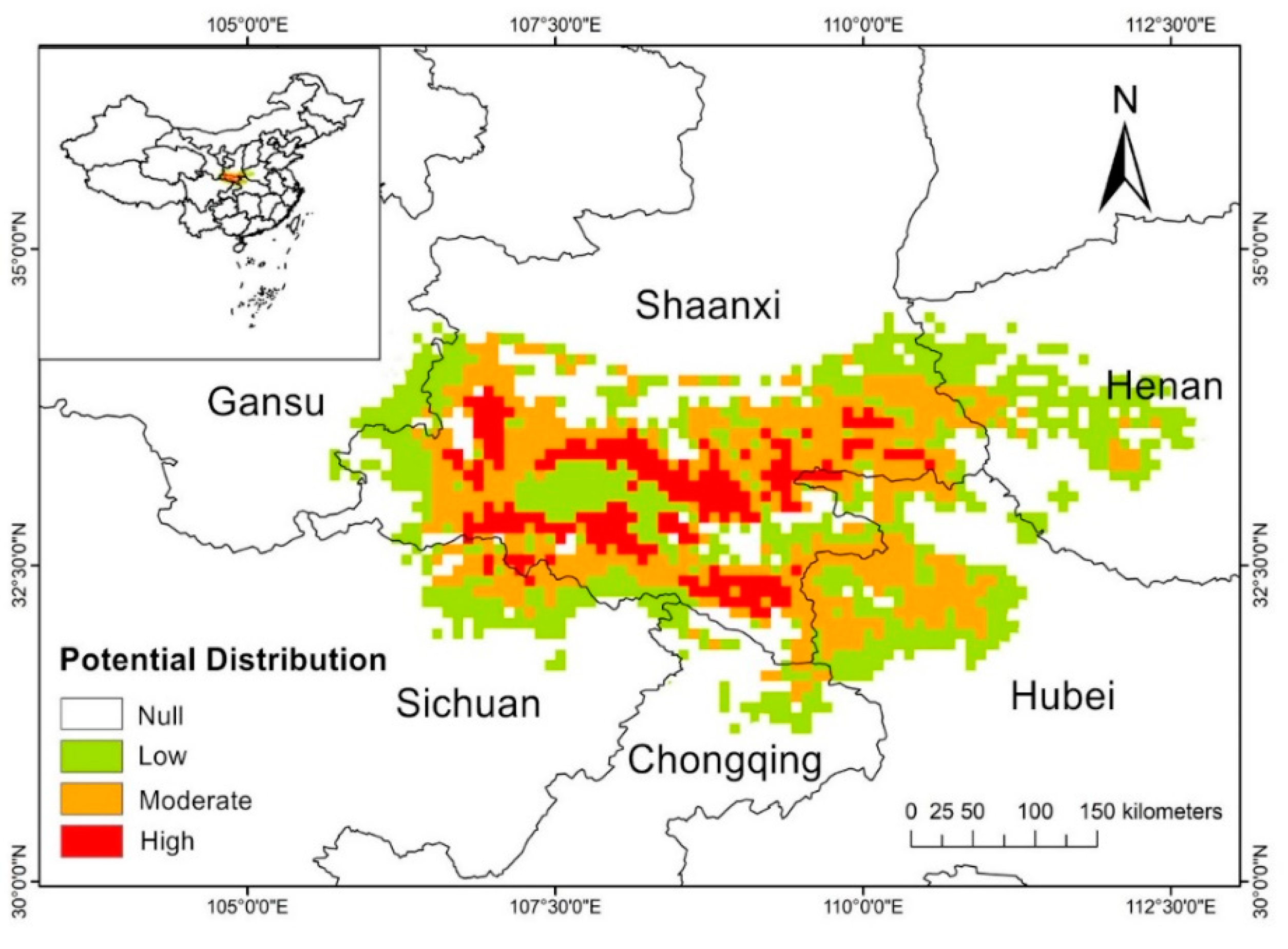
3.3. Potential Distribution of D. armandi Using SDMs
4. Discussion
5. Conclusions
Author Contributions
Funding
Acknowledgments
Conflicts of Interest
References
- Shaver, G.R. Spatial Heterogeneity: Past, Present, and Future. In Ecosystem Function in Heterogeneous Landscape; Lovett, G.M., Jones, C.G., Eds.; Springer: New York, NY, USA, 2005; pp. 443–449. [Google Scholar]
- Vinatier, F.; Tixier, P.; Duyck, P.F.; Lescourret, F. Factors and mechanisms explaining spatial heterogeneity: A review of methods for insect populations. Methods Ecol. Evol. 2011, 2, 11–22. [Google Scholar] [CrossRef]
- Brown, J.H. On the relationship between abundance and distribution of species. Am. Nat. 1984, 124, 255–279. [Google Scholar] [CrossRef]
- Thomas, C.D.; Bodsworth, E.J.; Wilson, R.J.; Simmons, A.D.; Davies, Z.G. Ecological and evolutionary processes at expanding range margins. Nature 2001, 411, 577–581. [Google Scholar] [CrossRef]
- Buckley, H.L.; Hannah, L.; Freckleton, R.P. Understanding the role of species dynamics in abundance-occupancy relationships. J. Ecol. 2010, 98, 645–658. [Google Scholar] [CrossRef] [Green Version]
- MacDonald, G.M. Biogeography: Introduction to Space, Time and Life. Prof. Geogr. 2010, 55, 283–285. [Google Scholar]
- Rodríguez, J.; Brotons, L.; Bustamante, J.; Seoane, J. The application of predictive modeling of species distribution to biodiversity conservation. Divers. Distrib. 2007, 13, 243–251. [Google Scholar] [CrossRef]
- Kearney, M.; Porter, W. Mechanistic niche modelling: combining physiological and spatial data to predict species’ ranges. Ecol. Lett. 2009, 12, 334–350. [Google Scholar] [CrossRef] [Green Version]
- Matern, A.; Drees, C.; Kleinwächter, M.; Assmann, T. Habitat modelling for the conservation of the rare ground beetle species Carabus variolosus (Coleoptera, Carabidae) in the riparian zones of headwaters. Biol. Conserv. 2007, 136, 618–627. [Google Scholar] [CrossRef]
- Srivastava, V.; Griess, V.C.; Padalia, H. Mapping invasion potential using ensemble modelling. A case study on Yushania maling in the Darjeeling Himalayas. Ecol. Modell. 2018, 385, 35–44. [Google Scholar]
- Miller, J. Species distribution modeling. In Geography Compass; Mike, B., Ed.; Wiley: Hoboken, NJ, USA, 2010; pp. 490–509. [Google Scholar]
- Pearson, R.G.; Dawson, T. Predicting the impacts of climate change on the distribution of species: Are bioclimate envelope models useful? Glob. Ecol. Biogeogr. 2003, 12, 361–371. [Google Scholar] [CrossRef]
- Beaumont, L.J.; Hughes, L.; Poulsen, M. Predicting species distributions: use of climatic parameters in BIOCLIM and its impact on predictions of species’ current and future distributions. Ecol. Model. 2005, 186, 251–270. [Google Scholar] [CrossRef]
- Elith, J.; Franklin, J. Species Distribution Modeling. In Encyclopedia of Biodiversity (Second Edition); Simon, A.L., Ed.; Academic Press: Waltham, MA, USA, 2013; pp. 692–705. [Google Scholar]
- Booth, T.H. Why understanding the pioneering and continuing contributions of BIOCLIM to species distribution modelling is important. J. Austral. Ecol. 2018, 43, 852–860. [Google Scholar] [CrossRef]
- Giusti, M.; Bo, M.; Angiolillo, M.; Cannas, R.; Cau, A. Habitat preference of Viminella flagellum (Alcyonacea: Ellisellidae) in relation to bathymetric variables in southeastern Sardinian waters. Cont. Shelf Res. 2017, 138, 41–45. [Google Scholar] [CrossRef]
- Palfreyman, J.; Graham-Brown, J.; Caminade, C.; Gilmore, P.; Otranto, D. Predicting the distribution of Phortica variegata and potential for Thelazia callipaeda transmission in Europe and the United Kingdom. Parasit Vectors 2018, 11, 272. [Google Scholar] [CrossRef]
- Van Gils, H.; Westinga, E.; Carafa, M.; Antonucci, A.; Ciaschetti, G. Where the bears roam in Majella National Park, Italy. J. Nat. Conserv. 2014, 22, 23–34. [Google Scholar] [CrossRef]
- Huang, M.; Ge, X.; Shi, H.; Tong, Y.; Shi, J. Prediction of Current and Future Potential Distributions of the Eucalyptus Pest Leptocybe invasa (Hymenoptera: Eulophidae) in China Using the CLIMEX Model. Pest Manag. Sci. 2019. [Google Scholar] [CrossRef] [PubMed]
- Chen, H.; Tang, M. Spatial and Temporal Dynamics of Bark Beetles in Chinese White Pine in Qinling Mountains of Shaanxi Province, China. Environ. Entomol. 2007, 36, 1124–1130. [Google Scholar] [CrossRef] [PubMed]
- Dai, L.; Ma, M.; Wang, C.; Shi, Q.; Zhang, R. Cytochrome P450s from the Chinese white pine beetle, Dendroctonus armandi (Curculionidae: Scolytinae): Expression profiles of different stages and responses to host allelochemicals. Insect Biochem. Mol. Biol. 2015, 65, 35–46. [Google Scholar] [CrossRef] [PubMed]
- Wang, D.; Liu, J.; Li, D.; Lei, R.; Lan, G. Community characteristics of Pinus armandi forest on Qinling Mountains. J. Appl. Ecol. 2004, 15, 357–362. [Google Scholar]
- Zhang, B.S. Geomorphology of the Qinling mountains. J. Northwest. Univ. 1981, 1, 81–87. [Google Scholar]
- Duque-Lazo, J.; Navarro-Cerrillo, R. What to save, the host or the pest? The spatial distribution of xylophage insects within the Mediterranean oak woodlands of Southwestern Spain. For. Ecol. Manag. 2017, 392, 90–104. [Google Scholar]
- Buse, J.; Schröder, B.; Assmann, T. Modelling habitat and spatial distribution of an endangered longhorn beetle–a case study for saproxylic insect conservation. Biol. Conserv. 2007, 137, 372–381. [Google Scholar] [CrossRef]
- Lausch, A.; Fahse, L.; Heurich, M. Factors affecting the spatio-temporal dispersion of Ips typographus (L.) in Bavarian Forest National Park: A long-term quantitative landscape-level analysis. For. Ecol. Manag. 2011, 261, 233–245. [Google Scholar]
- Zhang, Y.; Cai, H. Geographical distribution and community ecological characteristics of P. armandi. Hunan For. Sci. T. 1989, 4, 5–8. [Google Scholar]
- Zi, S.; Xiong, P.; Ma, L. Preliminary study on the prevention and control of the Chinese white pine beetle in Qinling Mountains and Ta-pa Mountains. J. Green Sci. Technol. 2016, 5, 41–42. [Google Scholar]
- Cuellar, R.G.; Equihua, M.A.; Estrada, V.E.; Mendez, M.T.; Villa, C. Fluctuacion poblacional de Dendroctonus mexicanus Hopkins (Coleoptera: Curculionidae: Scolytinae) atraidos a trampas en el noroeste de Mexico y correlation con variables climaticas. Boletin del Museo de Entomologia de la Universidad del Valle 2012, 13, 12–19. [Google Scholar]
- Hijmans, R.J.; Cameron, S.E.; Parra, J.L. Very high resolution interpolated climate surfaces for global land areas. Int. J. Climatol. 2005, 25, 1965–1978. [Google Scholar] [CrossRef] [Green Version]
- Naimi, B.; Skidmore, A.K.; Groen, T.A.; Hamm, N.A. Spatial autocorrelation in predictors reduces the impact of positional uncertainty in occurrence data on species distribution modelling. J. Biogeogr. 2011, 38, 1497–1509. [Google Scholar] [CrossRef]
- Graham, M.H. Confronting multicollinearity in ecological multiple regression. Ecology 2003, 84, 2809–2815. [Google Scholar] [CrossRef]
- Salinas-Moreno, Y.; Ager, A.; Vargas, C.F.; Hayes, J.L.; Zúñiga, G. Determining the vulnerability of Mexican pine forests to bark beetles of the genus Dendroctonus Erichson (Coleoptera: Curculionidae: Scolytinae). For. Ecol. Manag. 2010, 260, 52–61. [Google Scholar] [CrossRef]
- Allouche, O.; Tsoar, A.; Kadmon, R. Assessing the accuracy of species distribution models: prevalence, kappa and the true skill statistic (TSS). J. Appl. Ecol. 2006, 43, 1223–1232. [Google Scholar] [CrossRef] [Green Version]
- Hanley, J.A.; McNeil, B.J. The meaning and use of the area under a receiver operating characteristic (ROC) curve. Radiology 1982, 143, 29–36. [Google Scholar] [CrossRef]
- Jiménez-Valverde, A. Insights into the area under the receiver operating characteristic curve (AUC) as a discrimination measure in species distribution modelling. Glob. Ecol. Biogeogr. 2012, 21, 498–507. [Google Scholar] [CrossRef]
- Hirzel, A.H.; Hausser, J.; Chessel, D.; Perrin, N. Ecological-Niche Factor Analysis: How to Compute Habitat-Suitability Maps without Absence Data? Ecology 2002, 83, 2027–2036. [Google Scholar] [CrossRef]
- Hirzel, A.H.; Lay, G.L.; Helfer, V.; Randin, C.; Guisan, A. Evaluating the ability of habitat suitability models to predict species presences. Ecol. Model. 2006, 199, 142–152. [Google Scholar] [CrossRef]
- Hortal, J.; Roura-Pascual, N.; Sanders, N.J.; Rahbek, C. Understanding (insect) species distributions across spatial scales. Ecography 2010, 33, 51–53. [Google Scholar] [CrossRef]
- Anderson, R.P.; Lew, D.; Peterson, A.T. Evaluating predictive models of species’ distributions: criteria for selecting optimal models. Ecol. Model. 2003, 162, 211–232. [Google Scholar] [CrossRef] [Green Version]
- Lindenmayer, D.B.; Nix, H.A.; Mcmahon, J.P.; Hutchinson, M.F.; Tanton, M.T. The Conservation of Leadbeater’s Possum, Gymnobelideus leadbeateri (McCoy): A Case Study of the Use of Bioclimatic Modelling. J. Biogeogr. 1991, 18, 371–383. [Google Scholar] [CrossRef]
- Carroll, A.L.; Taylor, S.W.; Régnière, J.; Safranyik, L. Effect of climate change on range expansion by the mountain pine beetle in British Columbia. In Mountain Pine Beetle Symposium: Challenges and Solutions; Shore, T.L., Brooks, J.E., Eds.; Infromation Report BC-X.-399; Natural Resources Canada: Victoria, BC, Canada, 2003; p. 298. [Google Scholar]
- Mendoza, M.G.; Salinas-Moreno, Y.; Olivo-Martínez, A.; Zúñiga, G. Factors influencing the geographical distribution of Dendroctonus rhizophagus (Coleoptera: Curculionidae: Scolytinae) in the Sierra Madre Occidental, Mexico. Environ. Entomol. 2011, 40, 549–559. [Google Scholar] [CrossRef]
- Ungerer, M.J.; Ayres, M.P.; Lombardero, M.J. Climate and the northern distribution limits of Dendroctonus frontalis Zimmermann (Coleoptera: Scolytidae). J. Biogeogr. 1999, 26, 1133–1145. [Google Scholar] [CrossRef]
- Bentz, B.J.; Régnière, J.; Fettig, C.J.; Hansen, E.M.; Hayes, J.L. Climate change and bark beetles of the western United States and Canada: direct and indirect effects. BioScience 2010, 60, 602–613. [Google Scholar] [CrossRef]
- Økland, B.; Berryman, A. Resource dynamic plays a key role in regional fluctuations of the spruce bark beetles Ips typographus. Agric. For. Entomol. 2004, 6, 141–146. [Google Scholar] [CrossRef]
- Wang, X.; Zhang, Z.; Yang, W. Preliminary study on the biological characteristics of Dendroctonus armandi (Coleoptera: Curculionidae: Scolytinae). Sichuan For. Sci. Technol. 2014, 35, 56–58. [Google Scholar]
- Wang, J.; Gao, G.; Zhang, R.; Dai, L.; Chen, H. Metabolism and cold tolerance of Chinese white pine beetle Dendroctonus armandi (Coleoptera: Curculionidae: Scolytinae) during the overwintering period. Agric. For. Entomol. 2017, 19, 10–22. [Google Scholar] [CrossRef]
- Bale, J.S.; Masters, G.J.; Hodkinson, I.D.; Awmack, C.; Bezemer, T.M. Herbivory in global climate change research: direct effects of rising temperature on insect herbivores. Glob. Chang. Biol. 2002, 8, 1–16. [Google Scholar] [CrossRef]
- Wang, J.; Zhang, R.R.; Gao, G.Q.; Ma, M.Y.; Chen, H. Cold tolerance and silencing of three cold-tolerance genes of overwintering Chinese white pine larvae. Sci. Rep. 2016, 6, 34698. [Google Scholar] [CrossRef] [Green Version]
- Jaworski, T.; Hilszczański, J. The effect of temperature and humidity changes on insects development their impact on forest ecosystems in the expected climate change. For. Res. Pap. 2013, 74, 345–355. [Google Scholar] [CrossRef] [Green Version]
- Wang, X.L.; Chen, H.; Ma, C.; Li, Z. Chinese white pine beetle, Dendroctonus armandi (Coleoptera: Scolytinae), population density and dispersal estimated by mark-release-recapture in Qinling Mountains, Shaanxi, China. Appl. Entomol. Zool. (Jpn.) 2010, 45, 557–567. [Google Scholar] [CrossRef]
- Bjornstad, O.N.; Mikko, P.; Liebhold, A.M.; Werner, B. Waves of larch budmoth outbreaks in the European Alps. Science 2002, 298, 1020–1023. [Google Scholar] [CrossRef] [PubMed]
- Ims, R.A.; Leinaas, H.P.; Coulson, S. Spatial and temporal variation in patch occupancy and population density in a model system of an arctic Collembola species assemblage. Oikos 2010, 105, 89–100. [Google Scholar] [CrossRef]
- Giroday, H.M.C.D.L.; Carroll, A.L.; Lindgren, B.S.; Aukema, B.H. Incoming! Association of landscape features with dispersing mountain pine beetle populations during a range expansion event in western Canada. Landsc. Ecol. 2011, 26, 1097–1110. [Google Scholar]
- Powers, J.S.; Sollins, P.; Harmon, M.E.; Jones, J.A. Plant-pest interactions in time and space: A Douglas-fir bark beetle outbreak as a case study. Landsc. Ecol. 1999, 14, 105–120. [Google Scholar] [CrossRef]
- Kolb, T.E.; Fettig, C.J.; Ayres, M.P.; Bentz, B.J.; Hicke, J.A. Observed and anticipated impacts of drought on forest insects and diseases in the United States. For. Ecol. Manag. 2016, 380, 321–334. [Google Scholar] [CrossRef]
- Mattson, W.J.; Haack, R.A. The role of drought in outbreaks of plant-eating insects. BioScience 1987, 37, 110–118. [Google Scholar] [CrossRef]


| Climate Type | Longitude/Latitude | Environmental Overview | Distribution Range |
|---|---|---|---|
| North subtropical evergreen deciduous broad-leaved mixed forest belt | 29° N–33° N 105° E–111° E | The annual average temperature is 7–16 °C, the extreme minimum temperature is −5 to −22 °C, the extreme maximum temperature is 29–41 °C, the accumulated temperature of ≥10 °C is 2300–4500 °C, the annual precipitation is 1000–1400 mm. | The junction of Shannxi, Sichuan, Gansu, Hubei, Chongqing and Henan provinces in southern the Qinling Mountains, including Ta-ba Mountains, Micang Mountains and Wushan Mountains. |
| Central subtropical evergreen broad-leaved forest belt | 24° N–29° N 98° E–105° E | The annual average temperature is 10.5–18.3 °C, the extreme minimum temperature is −1.7 to −13.8 °C, the extreme maximum temperature is 33.8 °C, the accumulated temperature of ≥10 ℃ is 4500 to 5500 °C, the annual precipitation is 500–1400 mm. | Northeast and Northwest Yunnan, western Guizhou, and southwestern Sichuan. |
| Warm temperate deciduous broad-leaved forest belt | 33° N–36° N 105° E–113° E | The annual average temperature is 6–13 °C, the extreme minimum temperature is −18 to −24 °C, the extreme maximum temperature is 30–38 ℃, the accumulated temperature of ≥10 °C is 2000–4000 °C, the annual precipitation is 70–1000 mm. | All the distribution in northern the Qinling Mountains, include the southern the Zhongtiao Mountains in Shanxi, the Liupan Mountains in Ningxia, the Longshan in Gansu, the Funiu Mountains in Henan. |
| Code | Bioclimatic Variables | % Contribution |
|---|---|---|
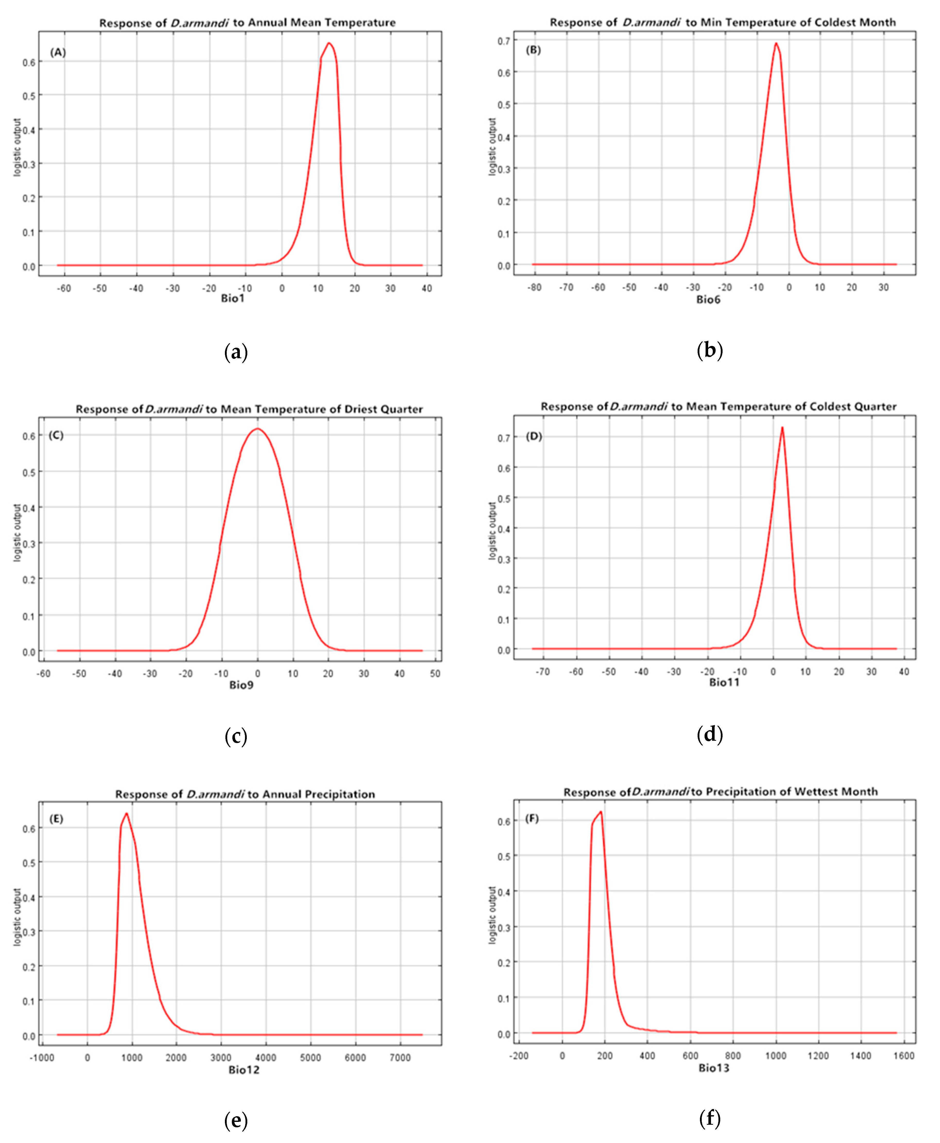
| Bio11 | Mean temp of coldest quarter (°C) | 25.6 |
| Bio9 | Mean temp of driest quarter (°C) | 15.3 |
| Bio6 | Minimum temp of coldest month (°C) | 14.1 |
| Bio1 | Annual mean temp (°C) | 11.5 |
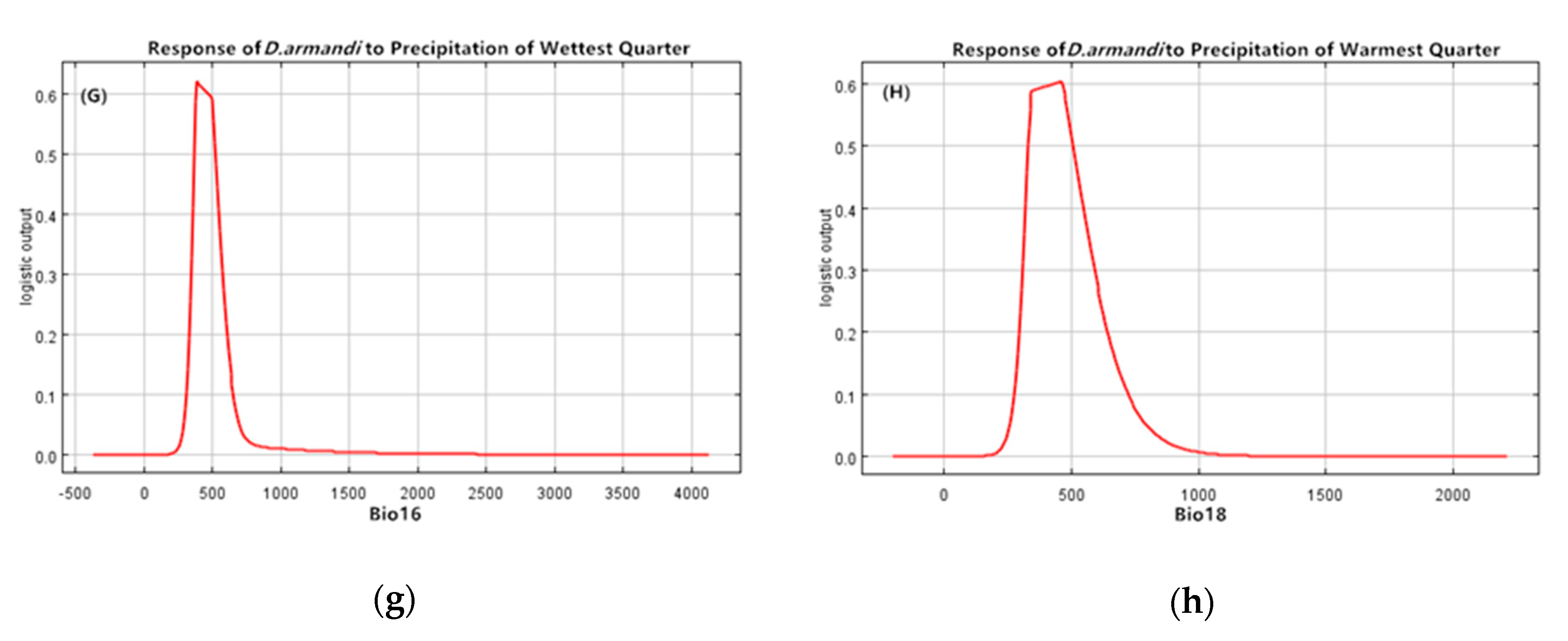
| Bio16 | Precipitation of wettest quarter (mm) | 10.8 |
| Bio18 | Precipitation of warmest quarter (mm) | 9.7 |
| Bio13 | Precipitation of wettest month (mm) | 8.6 |
| Bio12 | Annual precipitation (mm) | 4.5 |
| Title 1 | Climatic Variables | Eigenvalues | ||
|---|---|---|---|---|
| Component 1 | Component 2 | Component 3 | ||
| Bio1 a | Annual mean temp (°C) | 0.70 | 0.71 | −0.05 |
| Bio2 a | Mean diurnal range (°C) | −0.58 | 0.42 | 0.56 |
| Bio3 | Isothermality | −0.62 | −0.19 | 0.25 |
| Bio4 | Temperature seasonality | −0.16 | 0.76 | 0.51 |
| Bio5 | Maximum temp of warmest month (°C) | 0.51 | 0.83 | 0.20 |
| Bio6 a | Minimum temp of coldest month (°C) | 0.84 | 0.40 | −0.30 |
| Bio7 | Temperature annual range | −0.34 | 0.67 | 0.61 |
| Bio8 | Mean temp of wettest quarter (°C) | 0.63 | 0.77 | 0.05 |
| Bio9 a | Mean temp of driest quarter (°C) | 0.78 | 0.54 | −0.22 |
| Bio10 | Mean temp of warmest quarter (°C) | 0.59 | 0.80 | 0.03 |
| Bio11 a | Mean temp of coldest quarter (°C) | 0.78 | 0.54 | −0.02 |
| Bio12 a | Annual precipitation (mm) | 0.83 | −0.53 | 0.14 |
| Bio13 a | precipitation of wettest month (mm) | 0.86 | −0.34 | −0.11 |
| Bio14 a | precipitation of driest month (mm) | 0.75 | 0.42 | 0.49 |
| Bio15 | precipitation seasonality (mm) | −0.41 | 0.35 | −0.73 |
| Bio16 a | precipitation of wettest quarter (mm) | 0.82 | −0.47 | −0.17 |
| Bio17 | precipitation of driest quarter (mm) | 0.75 | −0.42 | 0.51 |
| Bio18 a | precipitation of warmest quarter (mm) | 0.84 | −0.46 | −0.07 |
| Bio19 | precipitation of coldest quarter (mm) | 0.75 | −0.42 | 0.51 |
| % Explained variance | 45.1 | 29.4 | 13.1 | |
| Province | Title 2 | Records (County & Forestry Bureau) |
|---|---|---|
| Shaanxi | 74 | Chang’an District, Huyi District, Zhouzhi, Zhashui, Zhen’an, Ningshan, Shiquan, Langao, Zhenping, Ziyang, Hanying, Foping, Liuba, Mian, Xixiang, Zhenba, Nanzheng, Ningqiang, Taibai, Feng, Mei, Ningxi Forestry Bureau, Ningdong Forestry Bureau, Changqing Forestry Bureau, Hanxi Forestry Bureau, Longcaoping Forestry Bureau, etc. |
| Gansu | 21 | Hui, Liangdang, Wen, Cheng, Kang, Xiaolongshan Forestry Experiment Bureau, etc. |
| Henan | 26 | Lingbao, Lushi, Luoning, Luanchuan, Songshan, Lushan, Nanzhao, Xixia, Xichuan, Neixiang, etc. |
| Sichuan | 17 | Chaotian District, Lizhou District, Wangcang, Jiange, Nanjiang, Tongjiang, Wanyuan City, etc. |
| Chongqing Municipality | 12 | Chengkou, Kaizhou District, Wuxi, Fengjie, Wushan, etc. |
| Hubei | 16 | Zhuxi, Zhushan, Yunxi, Baokang, Badong, Shennongjia Nature Reserve, etc. |
| Environmental Variables | Min. | Max. | Mean | SD | 5% | 10% | 50% | 90% | 95% |
|---|---|---|---|---|---|---|---|---|---|
| Annual mean temp (°C) | 5.6 | 17.1 | 11.6 | 2.7 | 7 | 7.5 | 12 | 15 | 15.3 |
| Mean diurnal range (°C) | 7 | 12 | 9.2 | 0.9 | 8 | 8 | 9 | 10 | 11 |
| Isothermality | 24 | 32 | 29.8 | 1.6 | 27 | 28 | 30 | 31 | 32 |
| Temperature seasonality | 718 | 970 | 792.8 | 55.6 | 728.9 | 735.8 | 782 | 885 | 902.3 |
| Maximum temp of warmest month (°C) | 21 | 33 | 26.4 | 3.1 | 22 | 22 | 26 | 31 | 32 |
| Minimum temp of coldest month (°C) | −11 | 2 | −4.6 | 2.8 | −10 | −9 | −4 | −1 | −1 |
| Temperature annual range | 28 | 38 | 31 | 2.3 | 29 | 29 | 30 | 34 | 36 |
| Mean temp of wettest quarter (°C) | 14 | 26 | 20.3 | 3.0 | 16 | 16 | 20 | 24 | 25 |
| Mean temp of driest quarter (°C) | −5 | 7 | 1.5 | 2.7 | −3.1 | −2.2 | 2 | 4 | 5 |
| Mean temp of warmest quarter (°C) | 15 | 27 | 21.2 | 3.1 | 16 | 17 | 21 | 25 | 26 |
| Mean temp of coldest quarter (°C) | −5 | 7 | 1.5 | 2.7 | −3.1 | −2.2 | 2 | 4 | 5 |
| Annual precipitation (mm) | 579 | 1286 | 910 | 181.9 | 671.8 | 695.8 | 878 | 1195.2 | 1248.8 |
| precipitation of wettest month (mm) | 118 | 232 | 165.8 | 28.1 | 127.9 | 132 | 159 | 204.4 | 211 |
| precipitation of driest month (mm) | 3 | 22 | 9.6 | 4.7 | 4 | 4 | 8 | 17 | 19 |
| precipitation seasonality (mm) | 63 | 94 | 72.2 | 6.7 | 64 | 65 | 72 | 81 | 83 |
| precipitation of wettest quarter (mm) | 301 | 564 | 436.2 | 66 | 348 | 362.8 | 423 | 524 | 544.6 |
| precipitation of driest quarter (mm) | 12 | 74 | 35.3 | 15.8 | 15 | 17 | 31 | 59 | 67 |
| precipitation of warmest quarter (mm) | 269 | 552 | 405.6 | 73.7 | 317.9 | 323 | 381 | 510 | 535.7 |
| precipitation of coldest quarter (mm) | 12 | 74 | 35.3 | 15.8 | 15 | 17 | 31 | 59 | 67 |
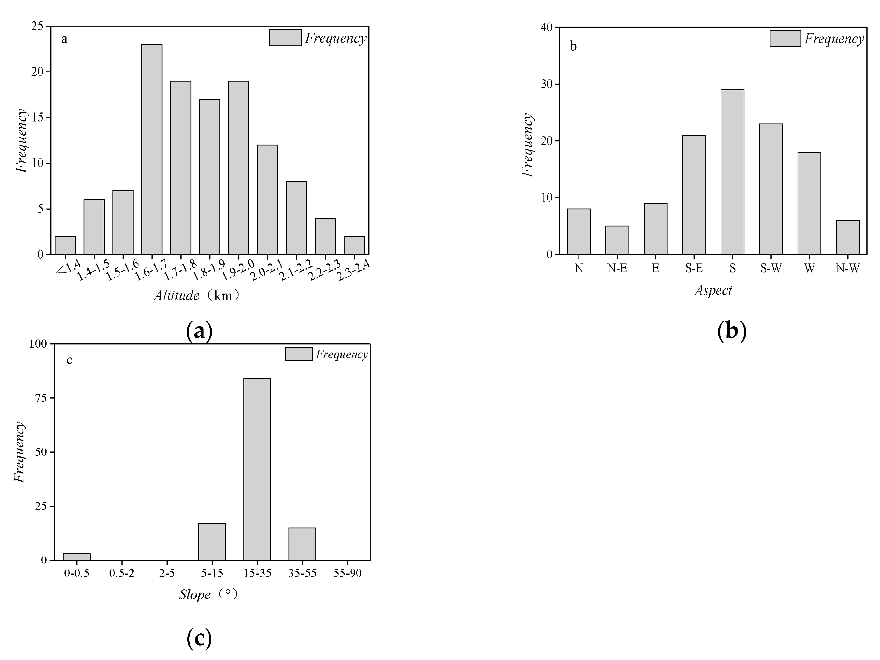
| Altitude (m a.s.l.) | 1323.5 | 2333.9 | 1815.9 | 213.9 | 1490 | 1559 | 1807 | 2114 | 2200 |
| Pinus Species | Incidence (%) |
|---|---|
| P. armandi Franch | 98.21 |
| P. tabulaeformis Carr. (Pinaceae) | 1.79 |
| P. massoniana Lamb. | 0 |
| P. bungeana Zucc. ex Endl. | 0 |
| Larix principis-rupprechtii Mayr | 0 |
| Category | Ecogeographic Variable (EGVs) | D. armandi | |||
|---|---|---|---|---|---|
| MF (100%) SF1 (28%) | SF2 (47.9%) | SF3 (9.4%) | SF4 (6.3%) | ||
| Climate | Annual mean temp | −0.269 * | −0.018 | −0.070 | −0.011 |
| Minimum temp of coldest month | −0.300 * | 0.027 | 0.015 | 0.000 | |
| Mean temp of driest quarter | −0.314 * | 0.084 | 0.206 * | 0.043 | |
| Mean temp of coldest quarter | −0.377 * | 0.177 * | −0.200 * | −0.210 * | |
| Annual precipitation | 0.211 * | 0.101 | −0.080 | −0.309 * | |
| Precipitation of wettest month | 0.234 * | 0.011 | 0.004 | 0.000 | |
| Precipitation of wettest quarter | 0.301 * | 0.036 | 0.157 * | 0.004 | |
| Precipitation of warmest quarter | 0.133 | 0.032 | 0.079 | 0.023 | |
| Terrain | Altitude | 0.201 * | 0.001 | 0.001 | 0.000 |
| Aspect | 0.176 * | 0.000 | 0.001 | 0.000 | |
| Slope | 0.153 * | 0.000 | 0.000 | 0.000 | |
| Host | P. armandi distribution | 0.171 * | −0.036 | −0.027 | 0.000 |
| Ecogeographic Variables | % Contribution |
|---|---|
| Mean temp of coldest quarter | 29.3 |
| Mean temp of driest quarter | 15.1 |
| Minimum temp of coldest month | 14.8 |
| Altitude | 12.6 |
| Precipitation of wettest quarter | 9.7 |
| Annual mean temp | 6.9 |
| Precipitation of warmest quarter | 5.5 |
| Precipitation of wettest month | 2.8 |
| Annual precipitation | 1.4 |
| Aspect | 1.1 |
| Slope | 0.8 |
| Host distribution | 0.1 |
© 2019 by the authors. Licensee MDPI, Basel, Switzerland. This article is an open access article distributed under the terms and conditions of the Creative Commons Attribution (CC BY) license (http://creativecommons.org/licenses/by/4.0/).
Share and Cite
Ning, H.; Dai, L.; Fu, D.; Liu, B.; Wang, H.; Chen, H. Factors Influencing the Geographical Distribution of Dendroctonus armandi (Coleoptera: Curculionidae: Scolytidae) in China. Forests 2019, 10, 425. https://doi.org/10.3390/f10050425
Ning H, Dai L, Fu D, Liu B, Wang H, Chen H. Factors Influencing the Geographical Distribution of Dendroctonus armandi (Coleoptera: Curculionidae: Scolytidae) in China. Forests. 2019; 10(5):425. https://doi.org/10.3390/f10050425
Chicago/Turabian StyleNing, Hang, Lulu Dai, Danyang Fu, Bin Liu, Honglin Wang, and Hui Chen. 2019. "Factors Influencing the Geographical Distribution of Dendroctonus armandi (Coleoptera: Curculionidae: Scolytidae) in China" Forests 10, no. 5: 425. https://doi.org/10.3390/f10050425
APA StyleNing, H., Dai, L., Fu, D., Liu, B., Wang, H., & Chen, H. (2019). Factors Influencing the Geographical Distribution of Dendroctonus armandi (Coleoptera: Curculionidae: Scolytidae) in China. Forests, 10(5), 425. https://doi.org/10.3390/f10050425