Article

Examining Naturogenic Processes and Anthropogenic Influences on Tree Growth and Development via Stem Analysis: Data Processing and Computational Analytics

Natural Resources Canada, Canadian Forest Service, Canadian Wood Fibre Centre, Sault Ste. Marie, ON P6A 2E5, Canada
Forests 2019, 10(12), 1058; https://doi.org/10.3390/f10121058
Submission received: 6 September 2019 / Revised: 8 November 2019 / Accepted: 13 November 2019 / Published: 21 November 2019
(This article belongs to the Section Forest Ecology and Management)

Abstract

:
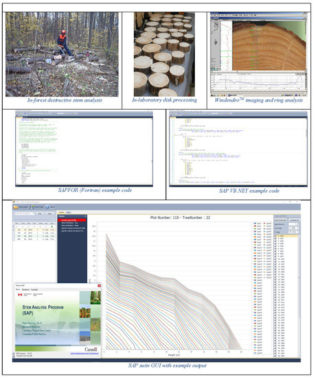
The objective of this study was to develop a stem analysis data processing and computational algorithm and associated software suite that was (1) applicable to temperate and boreal forest tree species, (2) mathematically consistent with excurrent tree stem geometric and allometric principles, (3) compatible with data structures obtained using proprietary and non-proprietary imaging systems, and (4) executable on Windows®-based operating systems. Computationally, the suite denoted SAP (Stem Analysis Program), deployed sectional-specific formulae that were in accord with the following geometric assumptions: (1) stump section was treated as a solid of revolution resembling a cylinder; (2) sections between the stump and the tip were treated as a solid of revolution resembling a frustum of a cone for sections with continuous annual increments, otherwise treated as a cone; and (3) tip section was treated as a solid of revolution resembling a cone. The algorithm also corrected for the slant-based sectional length measurements using Pythagorean Theorem and eliminated the requirement to predict age-specific apex height development through the use of a linear interpolation procedure. Based on input data structures consisting of annual ring-width xylem sequences measured from cross-sectional disk samples acquired at multiple positions along the tree’s main stem, the suite produces a broad array of output, inclusive of radial and longitudinal ring-width sequences, apical growth increments, annual and cumulative sectional and cumulative volume production patterns, and historically reconstructed stem taper profiles. In total, the SAP creates six output data files for each tree analyzed: (1) input data reference summary (e.g., geometric mean ring-widths and resultant radii for each cross-section); (2) radial growth patterns for the cross-section sampled at breast-height (e.g., absolute and relative diameter and basal area growth estimates); (3) sectional (vertical) profiles of volume growth patterns (e.g., absolute and relative growth estimates within each section (bolt)); (4) cumulative volume growth patterns for the entire tree; (5) historical taper profile estimates (e.g., heights and diameters by year); and (6) texturally-labeled compendium of all output files generated. Additionally, real-time graphical output was produced for the purposes of data assessment and verification during the radial sequence data acquisition stage (e.g., graphical presentation of annual ring-width sequences by radii and disk, for use in validating input data structures and increment measurements derived from the imaging system), and interpreting growth and development patterns (e.g., vertical growth layer and specific volume increment profiles by age or year). The utility of the SAP suite was exemplified by processing WindendroTM-based annual ring-width xylem sequences obtained from cross-sectional disks extracted from a jack pine (Pinus banksiana Lamb.) tree via percent-height destructive stem analysis, and subsequently elucidating growth and developmental patterns within the context of silviculture treatment effects (thinning). The SAP suite provides the conceptual and logistical foundation for the continued deployment of the stem analysis approach in a wide range of investigations, including those examining the effect of naturogenic processes and anthropogenic influences on tree growth and development.

Graphical Abstract

1. Introduction

Stem analysis, the demarcation and subsequent analysis of annual tree ring sequences that are encased within the main stem of temperate and boreal tree species, provides an analytical framework for examining naturogenic processes and anthropogenic effects on tree growth and development. As exemplified by numerous examples, stem analysis has been one of the principal approaches used in detecting and assessing historical growth and development patterns of excurrent tree species. Those examining naturogenic processes would include studies quantifying the effects of edaphic variation [1], resource competition [2], abiotic wind stress [3], insect defoliation [4], drought [5], and pathogens [6,7] on tree growth, whereas anthropogenic based investigations would include studies assessing tree growth responses to intensive forest management treatments, such as pre-commercial thinning [8] and commercial thinning [9], atmospheric pollution [10], and global warming [11]. Stem analysis has also been an essential tool for reconstructing ecological disturbance histories (e.g., [12,13,14]) and past climate variability within forest ecosystems (e.g., [15,16]). Furthermore, tree ring sequences have been used as terrestrial-based proxies in reconstructing past continental-scale temperatures and hydroclimatic changes in order to detect anthropogenic-generated climate change and quantifying the associated effects (e.g., [17,18]).
Contextually, stem analysis approaches could be categorized into one of three classes, based on the level of complexity deployed. The first level includes non-destructive approaches, where analyses are focused on the examination of radial annual-ring increment sequences extracted at a single stem position, e.g., at breast height (1.3 m), obtained from single or multiple sample tree(s), in order to draw inferences regarding temporal patterns of cross-sectional growth (e.g., diameter and basal area increments). The majority of research investigations within the fields of dendrochronology, dendroecology, dendroclimatology and dendrohydrology, which involve temperate and boreal forest tree species, could be classified as such (e.g., [19,20]). The standardization of data management protocols and methodologies in terms of cross-dating procedures and statistical approaches, inclusive of the provision of the prerequisite software analogues, are well developed for this analytical class (sensu Laboratory of Tree-Ring Research, University of Arizona, Tucson, AZ, USA). Furthermore, as a consequence, these approaches have received considerable acceptance and deployment, leading to the creation of well-populated open-access global repositories of standardized tree ring chronologies with pertinent metadata attached (e.g., International Tree-ring Data Bank [21]). Analysis of these data sets within the context of climate change have significantly advanced the understanding of the key drivers of tree growth, leading to more informed predictions of the consequences of anthropogenic-induced climate change across the globe (e.g., [22]). The second analytical class would include those approaches involving destructive stem analysis, where sample trees are felled and sectioned in order to obtain (1) radial annual-ring counts (cambial age) at multiple stem heights (e.g., branch nodes), so that that temporal height growth patterns of codominant and dominant trees can be reconstructed and subsequently quantified, yielding site index functions, or (2) outside cross-sectional diameters at multiple stem heights for examining and modeling stem taper and morphological-based allometric relationships. Numerous methodologies have also been established for this analytical class in terms of sampling designs, computational frameworks and biometrical modelling (e.g., [23,24,25,26]).
The third analytical class, which is the most informative and generally represents the “gold standard” in terms of analytical scope and inference potential, includes those approaches which attempt to reconstruct the entire growth and developmental tree-level histories through the acquisition of radial annual-ring increment sequences measured from multiple cross-sectional disks positioned at fixed or variable stem positions over the entire length of the main stem. Although this complete (whole tree) stem analysis approach is the most logistically and analytically challenging to apply, it does enable the 3-dimensional visualization of annual radial and vertical growth layer profiles, and consequently provides for an expanded inference space in terms of analyzing and interpreting the effects of intrinsic and extrinsic influences on temporal growth patterns, allometry and stem morphological development. The conceptual, analytical and inferential frameworks for the complete stem analysis approach were largely established through the efforts of a series of pioneering growth and morphological investigations of red pine (Pinus resinosa Ait.) in central Canada during the early 1950s to mid-1960s, by Duff and Nolan [27,28,29] and Forward and Nolan [30,31,32,33]. However, the computational burden of reconstructing temporal, radial and vertical patterns of tree growth and development from radial annual-ring increment sequences measured on multiple disks, can present a hindrance to its application in forest research investigations and operational forest management. Consequently, in order to potentially overcome this deterrent, the focus of this study was to present the prerequisite computational analytics and an associated software suite that was mathematically consistent with excurrent tree geometry, compatible with current software and hardware environments, and generated the response metrics that could facilitate comprehensive analyses of the effects of naturogenic processes and anthropogenic influences on tree growth and development.

2. Materials and Methods

2.1. Stem Analysis Computational Algorithm: Structure and Development

The VisualBasic.NET software suite, denoted SAP (Stem Analysis Program) herewith, was developed within the Visual Studio® development environment (VS.NET (Version 2012), Microsoft Inc. (MS), Redmond, WA, USA) and utilized a number of third party graphical and tabular reporting tools (i.e., ProEssentials (Version 6), GigaSoft Inc., Keller, TX, USA, and Input Pro for Windows Forms (Version 2.5), Charlotte, NC, USA, respectively). The main computational engine of the suite is the Fortran-based executable program, denoted SAPFOR.EXE (Stem Analysis Program – FORtran). SAPFOR is an improved and expanded version of the stem analysis algorithm previously presented by Newton [34,35]. Briefly, the SAPFOR program was written in Fortran using the Lahey/Fujitsu Fortran 95 compiler (www.lahey.com) and consisted of a main program and two subroutines. The primary function of the main program is to compute the geometric mean ring-widths and resultant radii, calendar date, and age from the raw data file, which consists of the annual ring width sequences from the multiple cross-sectional disk samples for a given sample tree. The first subroutine, denoted GDB for Growth Diameter and Basal area analysis, then computes radial growth estimates for the cross-section at breast-height, specifically. Subsequently, the second subroutine, denoted GVA for Growth Volume and Allometric analysis, computes the sectional and cumulative growth estimates, and stem developmental profiles. The underlying structure, computational assumptions, and mathematical formulae are detailed explicitly in Appendix A.
In terms of data processing, the suite also converts WinDendroTM-based (www.regentinstruments.com) Excel® input files (W3*.xlsx (Version 3 format) or W4*.xlsx (Version 4 format) into the required Fortran-based configuration for use within the SAPFOR. Specifically, the program processes the selected WinDendroTM-based Excel® input file by transcribing it into a 2-dimensional rectangle array format after removing (parsing) all extraneous data columns and infilling blank cells with null zero values, resulting in a correctly structured input file. Generically, the structure of the input file (denoted SWijklmn for Stem Width increments, where ijklmn is a numeric code for identifying the sample tree, and the plot and (or) stand it was sampled from) consists of the each disk’s height position (m) and its total age (years), followed by the cumulative length of the each radial sequence (mm or cm) and each annual ring-width increment (mm or cm) along each radii, starting from the pith and progressing outward to the outmost annual ring. Note that, as long as the increment data is presented in this structure, non-WindendroTM generated input files may also be processed by the program. Refer to input file SW11002.xlsx in Supplementary: Material S1 for an applicable example.
More specifically, employing radial xylem sequences derived from cross-sectional disks located at multiple sample points along the stem of excurrent (single-stem) forest tree species, the program calculates: (1) annual increments and one periodic increment for diameter and basal area growth at breast-height (1.3 m) in both absolute and relative terms; (2) annual volume increments and one periodic volume increment for each section in both absolute and relative terms; (3) annual increments and one periodic increment for volume growth in both absolute and relative terms for all sections combined; and (4) annual diameters and corresponding heights for each year. Note that the time interval pertaining to the periodic measurement is defaulted to unity, which in essence treats the periodic computation as an annual one. Currently, this option is included to enable further program expansion for addressing situations where (1) biotic or abiotic damage has resulted in partial disk samples, where all annual increment measurements along the radial sequence are not available (e.g., pathogenic incipient decay within the inner core) or (2) logistical limitations or study objectives dictate the annual measurement of only a fixed outer portion of the radial sequence (e.g., analyzing only post-treatment annual growth response patterns arising after the implementation of a mid-rotation silvicultural treatment).
Relative measures of growth included relative growth rate [36], growth percentage [37], specific volume increment [28], and relative production rate [38]. Relative growth rate and growth percentage express absolute growth as a proportion of initial size. Specific volume increment is defined as the rate of stem volume production per unit of stem surface area and, hence, indirectly reflects the ability of a tree to supply photosynthate (i.e., assimilates produced through photosynthesis) to the vascular cambium for xylem production. Relative production rate reflects the rate of change in stem volume growth between successive growth years. Conceptually, relative growth rate, growth percentage, specific volume increment and relative production rate, attempt to remove the effect of cumulative tree size, thus providing an unbiased method to assess growth performance among sample trees, irrespective of their size differences.

2.2. Exemplification of the Utility of the Resultant SAP Suite

In order to demonstrate the utility of the SAP suite, the processing of the annual ring-width increment sequences obtained from cross-sectional disks obtained from a jack pine (Pinus banksiana Lamb.) sample tree, and the associated analysis of the derived growth layer and specific volume increment profiles, are examined within the context of (1) identifying intrinsic developmental patterns generic to excurrent tree species, and (2) examining longitudinal growth responses to thinning treatments. Silviculturally, the selected sample tree had grown in a natural-origin, even-aged, monospecific (> 90% jack pine by basal area) stand that had been established via natural seeding in the year following a wildfire in 1945. The stand was located in the Tyrol Research Forest, which falls within the Nipigon Forest Section (B.10) of the Canadian Boreal Forest [39]. The stand was situated on a dry-to-moderately fresh sandy-textured conifer site type (ES 13 [40]) and was above-average in terms of its productivity (site index = 19 m [41]). In 1962, the stand was subjected to an operational precommercial thinning treatment when the sample tree was 17 years of age. This treatment reduced the stand density from approximately 8500 stems/ha to 2419 stems/ha (nominal 2.0 × 2.0 m spacing). Thirty-five years later, the stand was subjected to an experimental thinning treatment in 1997, when the sample tree was 52 years of age. This treatment reduced the stand density from approximately 1669 to 748 stems/ha (3.7 × 3.7 m nominal spacing). At the individual tree level, this treatment reduced the number of immediate competitors (i.e., trees within a 3 m radius of the sample tree) from five relatively smaller and larger sized (height-based) competitors down to two smaller sized competitors. Stand-level mensurational parameters at the time of the stem analysis sampling (autumn 2015) for stand density, quadratic mean diameter, mean dominant height, basal area, total volume, merchantable volume and relative density were, respectively: 622 stems/ha (4.0 × 4.0 m nominal spacing), 21.7 cm, 24.6 m, 23.07 m2/ha, 268.6 m3/ha, 252.2 m3/ha and 0.70. Tree-level measurements at time of sampling indicated that the selected sample tree had diameter at breast height (1.3 m), total height and live crown ratio values of 22 cm, 22 m and 29%, respectively.
In-forest stem analysis sampling procedures consisted of felling, delimbing, measuring for crown length and total stem length, and subsequently sectioning the main stem at the following height positions: stump (0.3 m), breast-height, and at 10% height intervals (10, 20,…,90). A cross-sectional disk was then removed from each of these positions, yielding a total of 11 disks. The section lengths were measured and the disks were then returned to cold storage until laboratory processing. In-laboratory procedures for each disk consisted of (1) sanding its cross-sectional surface, and (2) determining and marking its geometric mean diameter from which two annual ring width radial sequences were measured via the WindendroTM imaging system (Version 2012b; www.regentinstruments.com). The raw data files were saved in the Version 4 format (denoted W411002.xlsx; see Supplementary Material S1). In order to demonstrate the SAP suite employing all three possible input data file configurations, a WindendroTM Version 3 file and a SW data file, were also created (denoted W311002.xlsx and SW11002.xlsx, respectively; see Supplementary Material S1). Note, the file name (identifier) used for this example was 110022 (ijklmn) which indicated that the sample tree number was 022, sampled from plot number 110.

3. Results

3.1. Overview of the Resultant SAP Suite

Contextually, the SAP suite is a data-base driven MS Access application, consisting of a VB-based program in which input data files are assessed for their size parameters and subsequently manipulated in order to comply with the input requirements of the Fortran-based computational algorithm (SAPFOR). Consistent with widely accepted bole shape principles for excurrent tree species (sensu [42]), the SAPFOR-based computational formulae were based on the following geometric identities: (1) stump section was treated as a solid of revolution resembling a cylinder; (2) sections between the stump and the tip were treated as a solid of revolution resembling a frustum of a cone in cases where the annual increment was continuous throughout the section, or a cone in cases where the annual increment was not continuous throughout the section; and (3) tip section was treated as a solid of revolution resembling a cone. The algorithm also corrected for the slant-based sectional length measurements using Pythagorean Theorem and eliminated the need to predict height at a given age through the employment of a linear interpolation procedure. Based on input data structures consisting of annual ring-width xylem sequences measured from cross-sectional samples acquired at multiple positions along the main stem, the resultant suite produced a broad array of output, including radial and longitudinal ring-width sequences, apical growth increments, annual and cumulative sectional and cumulative volume production patterns, and historical stem developmental profiles. Graphics were also generated for data verification (e.g., evaluating the measured annual ring-width data by radii and disk) and interpreting temporal growth and developmental patterns (e.g., analyzing vertical growth layers and specific volume increment profiles by age or year).

3.2. Input File Format and Structure, Program Execution, and Generated Output

The input file containing the ring-width sequences must be formatted as a complete rectangular matrix with all cells populated if the input file is manually created from an imaging system other than WindendroTM. The required structure for manually inputted annual-ring sequences for each cross-sectional disk is the following: age of the kth cross-section (year); height of the kth cross-section (m); radial-specific ring-width sequences, each consisting of the total radial length (cm), and annual ring widths (mm) arranged in a pith-to-bark order. The order of the disks must also follow a specified pattern: sequences obtained from the stump cross-section, then the breast-height cross-section, then the sections between the breast-height and the tip ordered by increasing height, terminating with the tip section (refer to file SW11002.xlsx in the Supplementary Material S1 for an example of the correct structure). Otherwise, in the case of WindendroTM generated Excel® files, either in Version 3 or 4 format, the suite automatically completes this data management step. Specifically, it parses and rearranges the raw WindendroTM data files and then completes the necessary preliminary calculations resulting in the correctly structured SGijklmn.DAT (Stem Growth increment) input file. In terms of analytical scope, one to eight radial sequences per disk, and up to 16 cross-sectional disks per tree, can be accommodated.
Upon execution, the SAP suite creates six output data files which can be readily exported for further analysis: (1) GFijklmn.DAT (Geometric Formatted file), consisting of the geometric mean ring-widths and resultant radii for each cross-section; (2) BIijklmn.xlsx (Breast-height Increment data file), consisting of the diameter and basal area growth metrics for the breast-height cross-section only; (3) SSijklmn.xlsx (Stem Sectional data file), consisting of volume growth metrics for each section; (4) STijklmn.xlsx (Stem Total data file), consisting of the cumulative volume growth metrics based on all sections combined; (5) SFijklmn.xlsx (Stem Form data file), consisting of the historical reconstructed stem taper profiles by year; and (6) REijklmn.xlsx (REference data file), consisting of a labeled summary of all five files collated together. Graphics are also produced for data verification and preliminary growth analysis. Specifically, in terms of data verification, the actual increment widths by year for each radii on each disk are presented to assist the analyst in verifying the input data derived from the imaging system (e.g., graphical detection of outliers or incorrect measurements). An average trend line is also produced for each disk, in order to visually evaluate the general growth trends within and among disks. In terms of preliminary analyses and to aid interpretation, the growth layer and the specific volume increment profiles for the entire tree are also graphically illustrated.
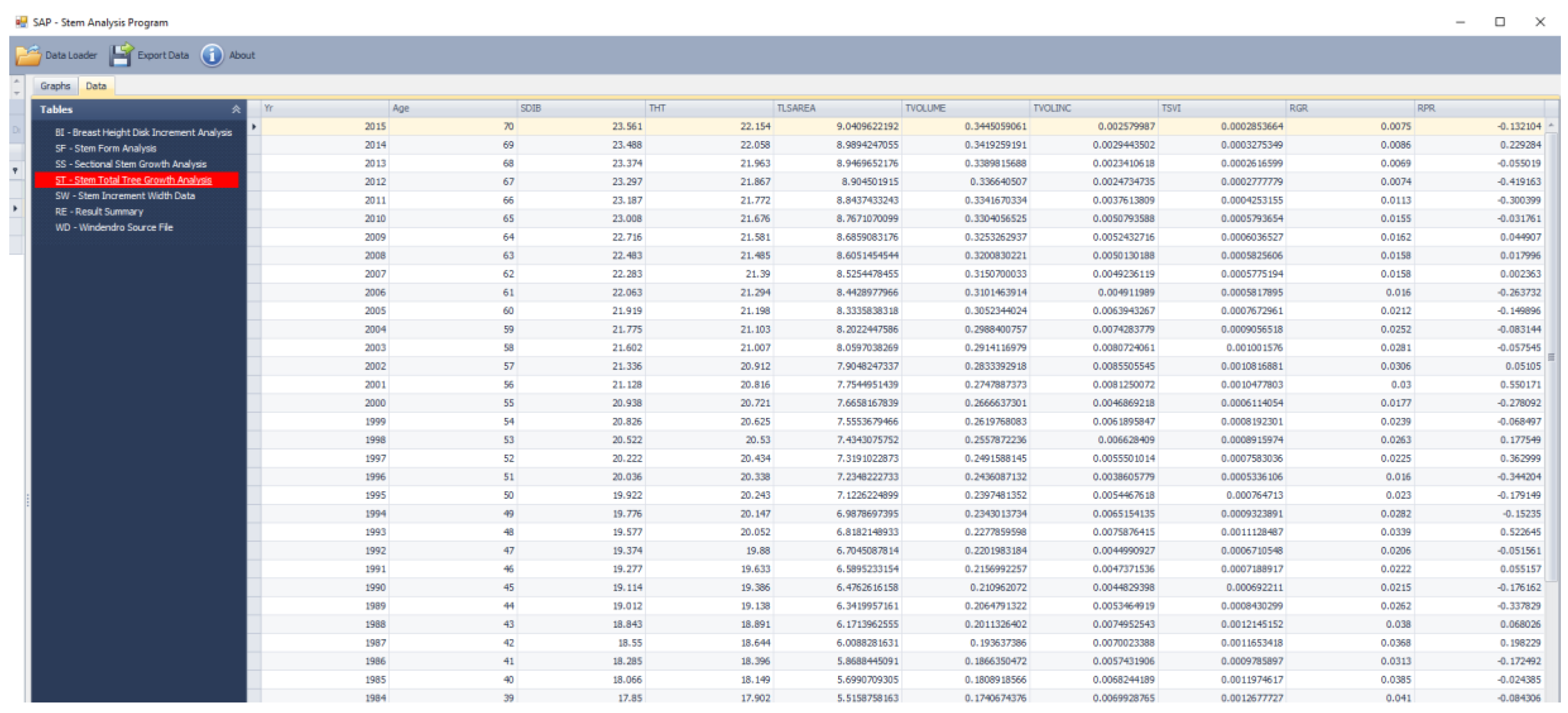
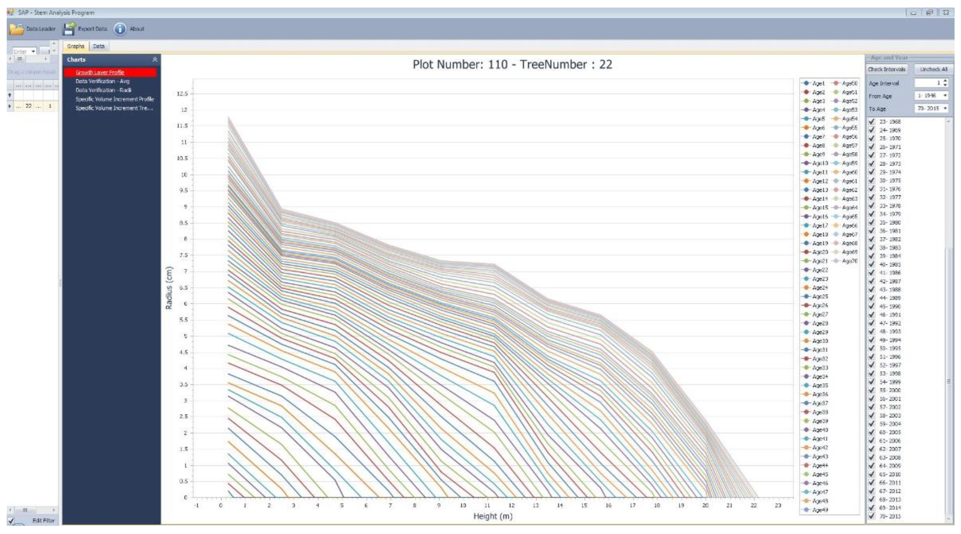
By way of example, in reference to the sample tree demonstration, the input files were placed in a separate computer directory and, upon execution of the SAP suite, loaded into the suite using the “Data Loader” tool bar (Figure 1). Note, the end-user must specify the (1) sampling year, (2) number of years for the periodic increment (currently the value is set to a default value of unity), (3) annual increment measurement units (cm or mm), and (4) identify the source folder (C:\Users\pnewton\Documents\SAP-BETA-EXEC\TESTTREE) and associated increment file (e.g., W4110022.xlsx). Following the selection of the input data file and setting the above parameters, the SAP suite provides the original source input file from the imaging system (e.g., W411002.xlsx) and its associated SAP-compatible reformatted input file, followed by the generated six output data files. Note, the RE110022.xlsx file which includes all 5 of the individual labelled output files is presented in the Supplementary Material S2. Within the SAP graphical user interface (GUI), all of these files are presented as a set of tables under the “Data” tool bar (Figure 2). The data verification, growth layer and specific volume increment profiles graphics are presented as a set of figures under the “Graph” tool bar (Figure 3). Additionally, for the profile graphs, end-users have the option of selecting increment profile illustrations for one or more of the years analyzed.

3.3. Interpretation Guidance and Related Inferences Derived

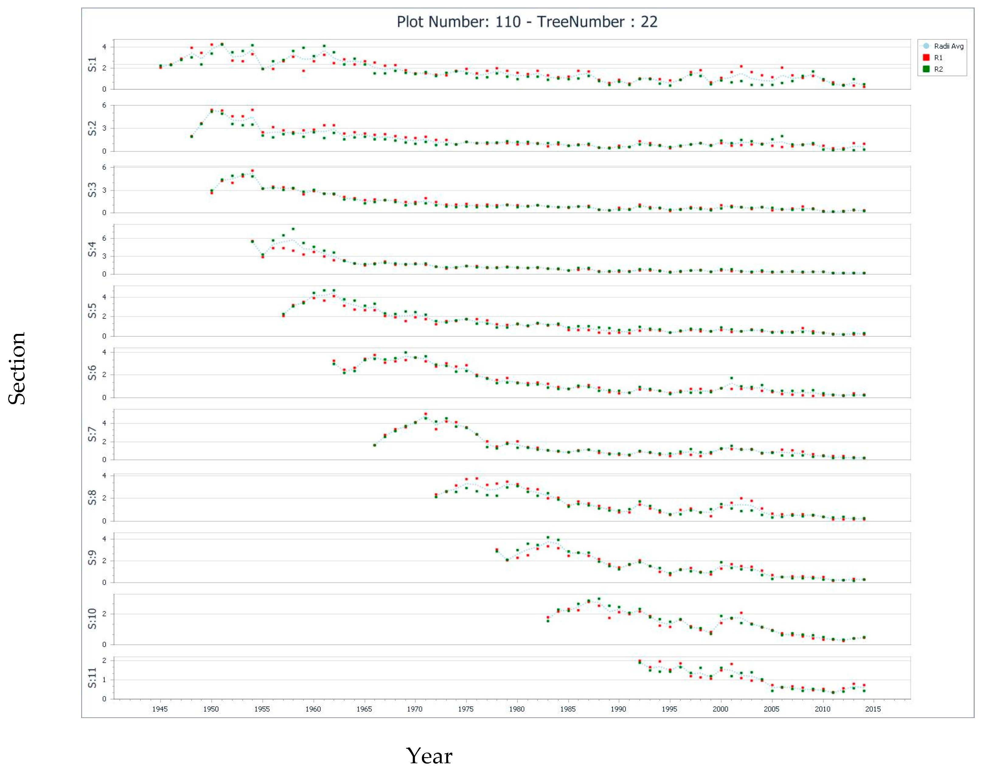
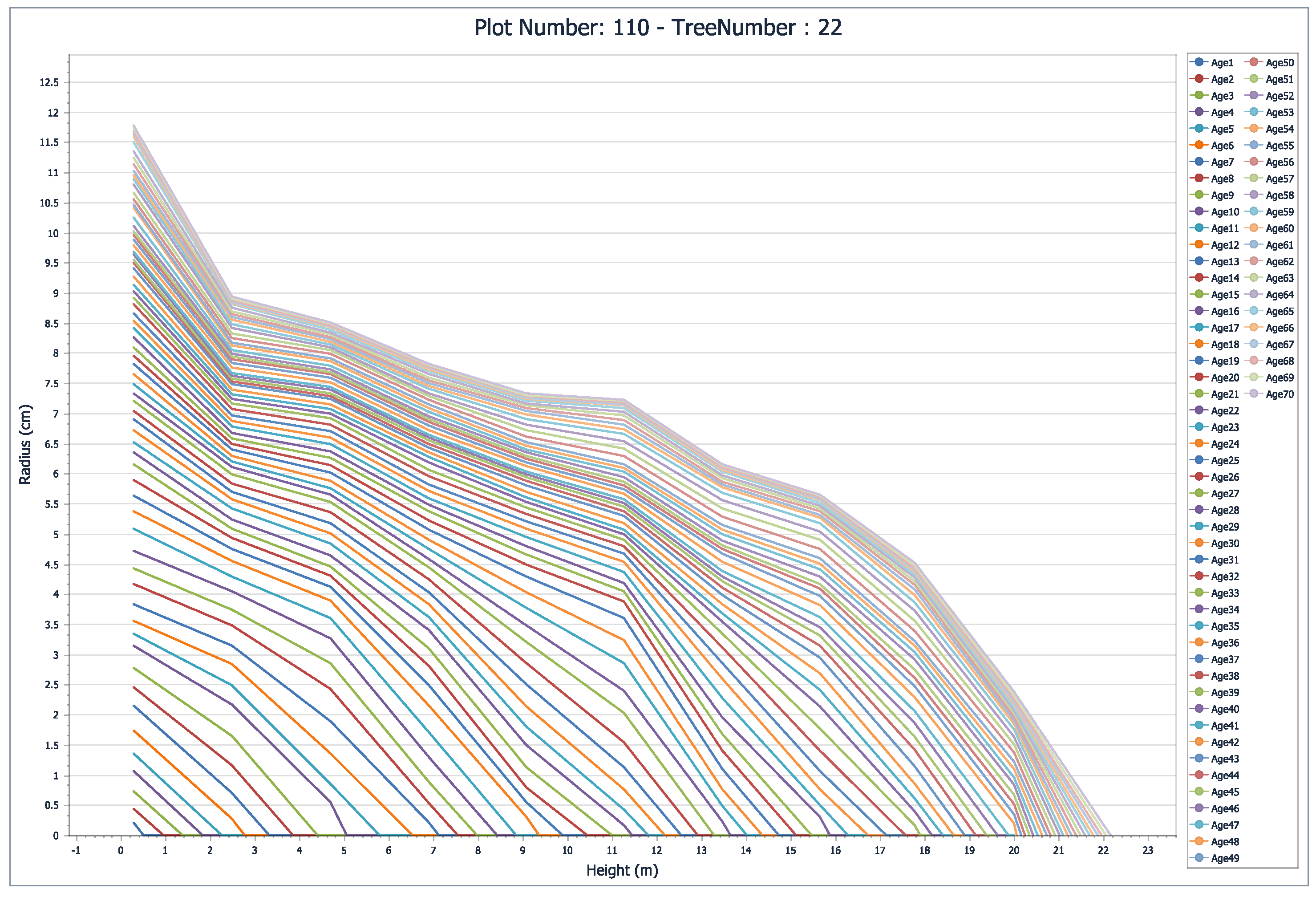
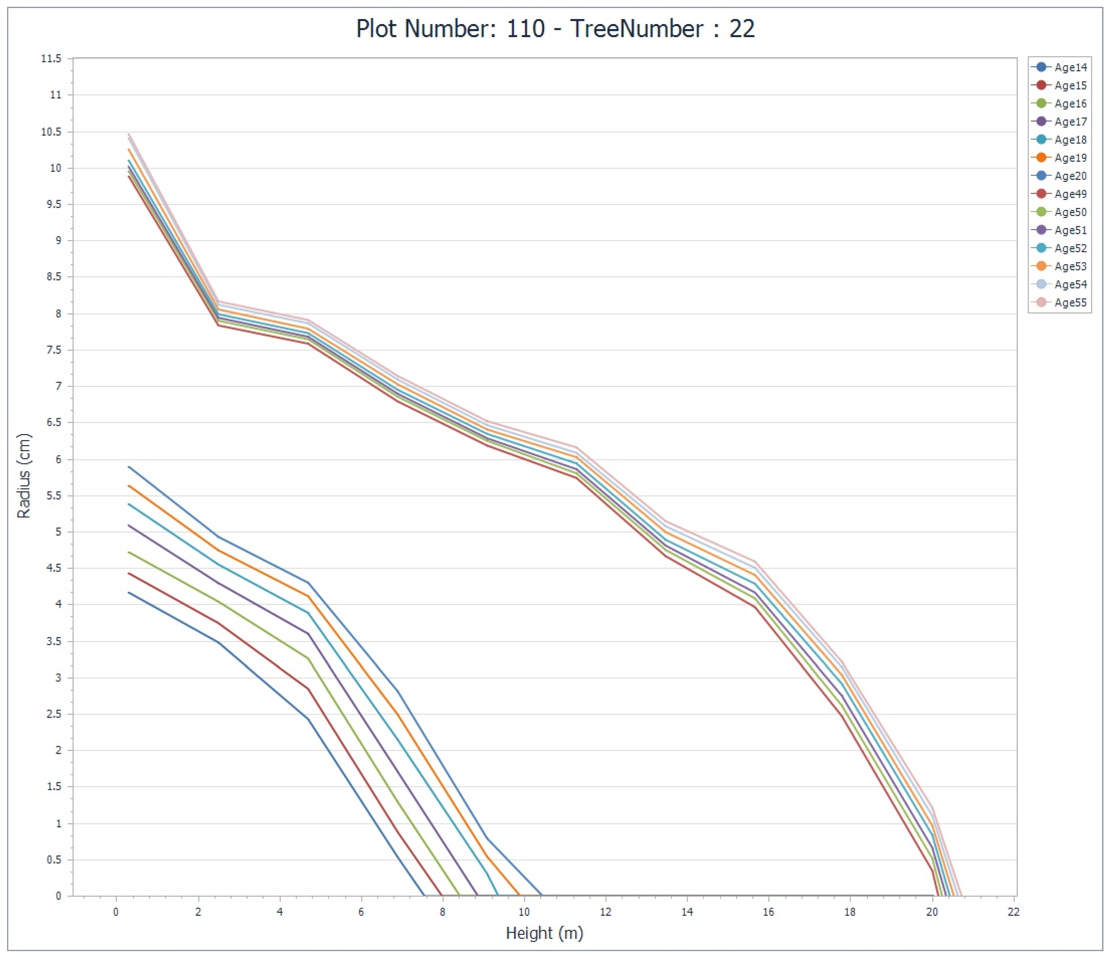
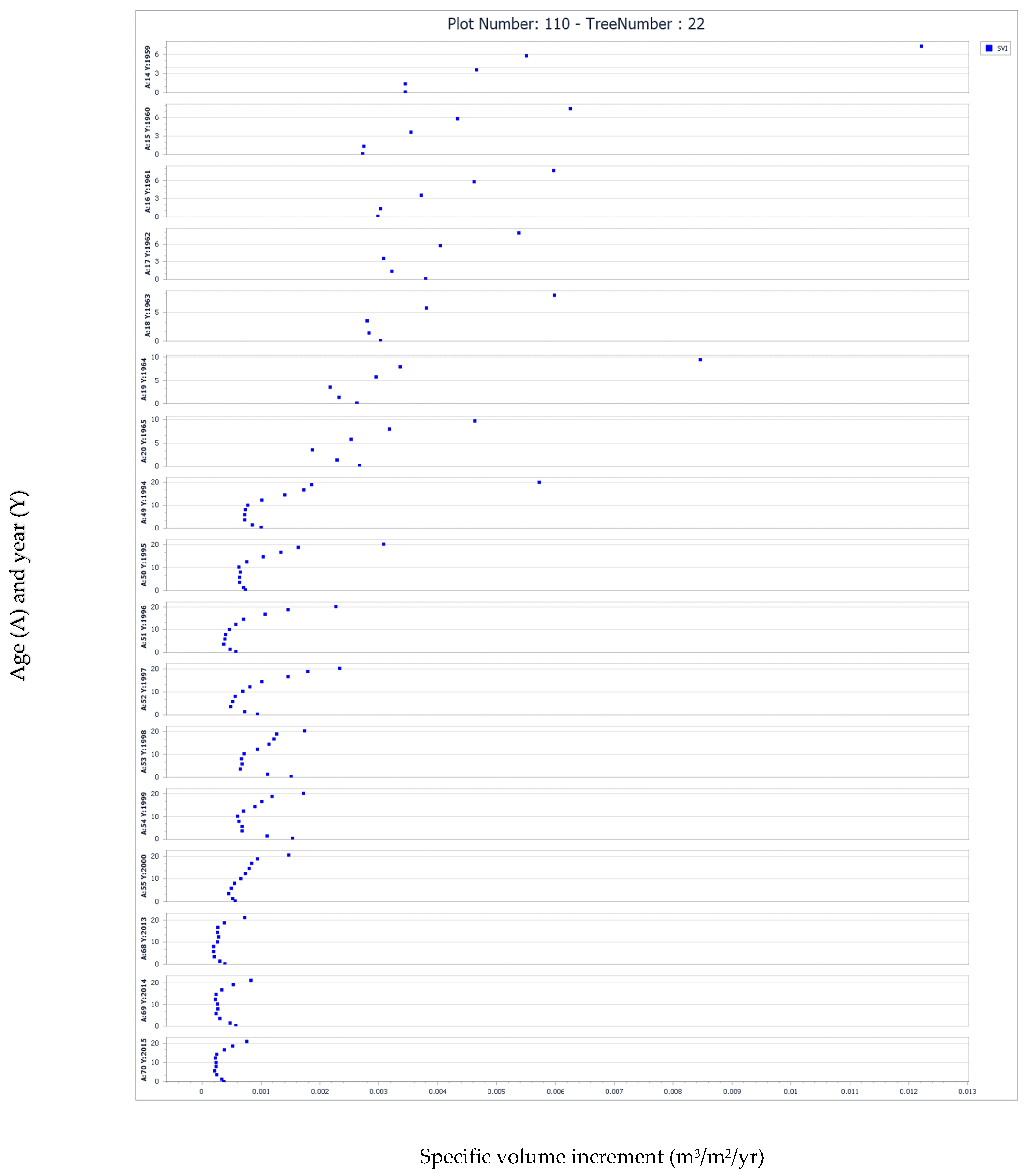
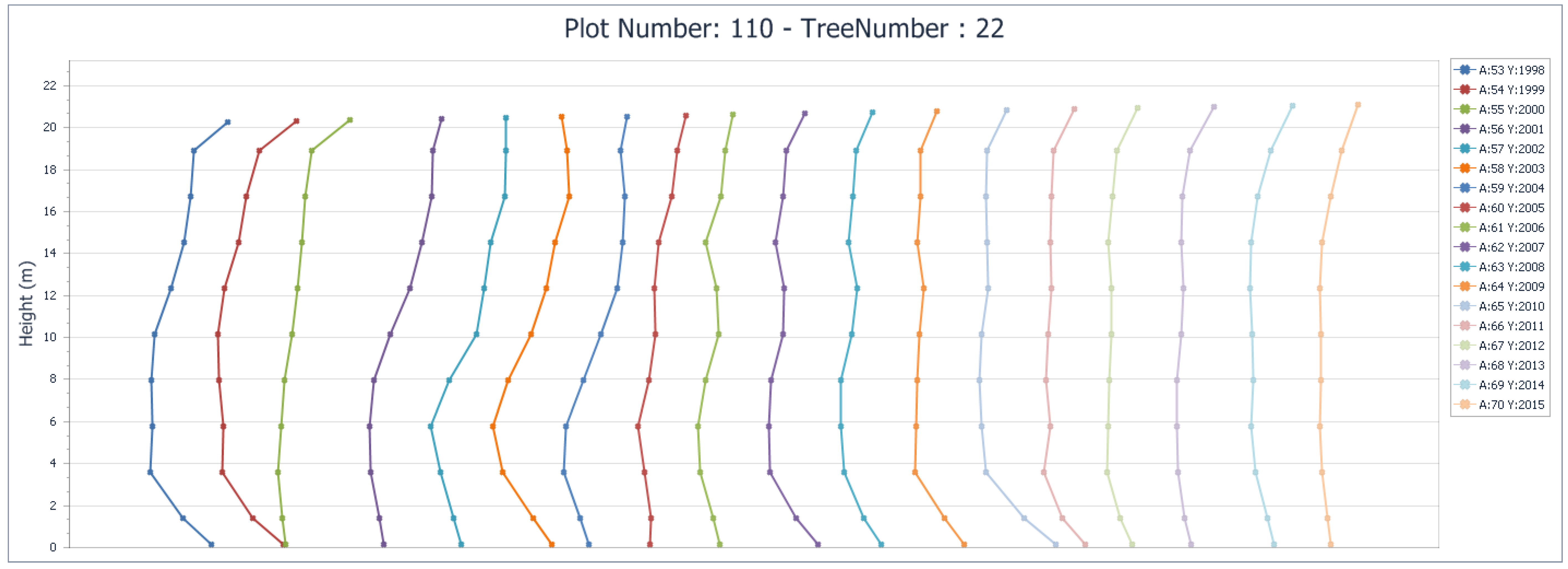
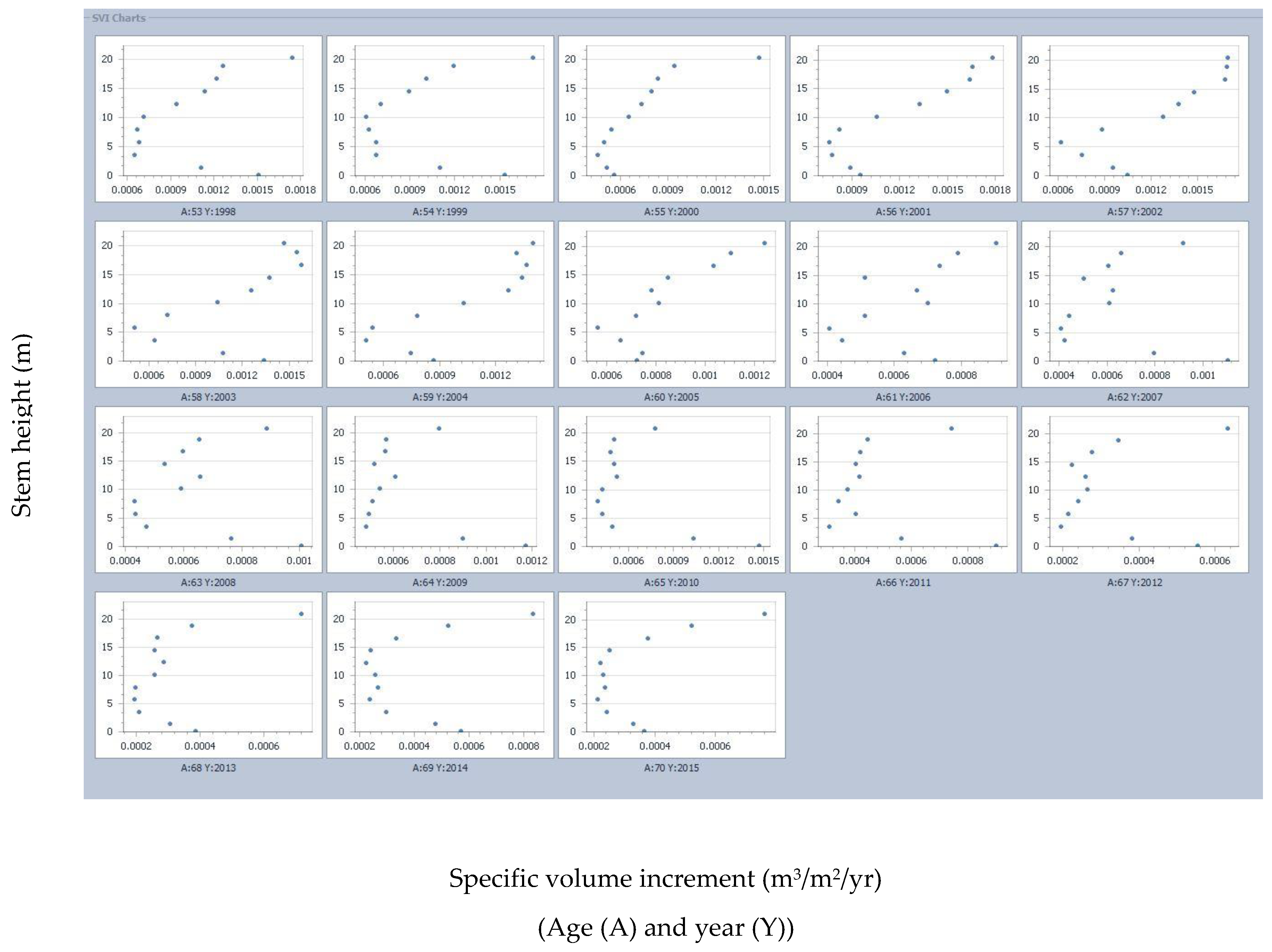
Figure 4 illustrates the actual increment widths by year for each of the two radii on each of the 11 disks obtained from the jack pine sample tree. Visual examination of the radius-specific increment values, along with the mean increment trend line by disk, revealed no discernable outliers in the raw increment data. The resultant growth layer profile for the tree is presented in Figure 5. The growth layer profiles were consistent with expectations: (1) for any given growth layer, the radial increment exhibited a general increase from the stump upwards and then declined rapidly as the apex was approached; empirically the maximum increment occurs at the 80% height percentile position, which corresponded to a point approximately 1/3 into the basal portion of the live crown, (2) as the tree aged, the point at which the radial increment was minimal occurred at a height of approximately 20%; and (3) although this increment profile pattern became more pronounced with age, presumably due to increasing intraspecific competition, the width of the radial increments temporally increased following the thinning treatments, particularly after the second thinning (Figure 6). These longitudinal increment patterns follow those espoused by Farrar [43]: i.e., (1) the point of the maximum increment occurring at the stem position where the crown density was the highest (assumed to occur at an 80% height percentile for the sample tree analyzed in this study), (2) the increment increasing from the apex to the mid-crown position, but thereafter declining with decreasing height until a minimum is approached (assumed to occur at a 20% height percentile for the sample tree analyzed in this study), and (3) increments then slightly increasing from that point until the base of the tree is reached. This increase in the lower bole (stump region) has been associated with mechanical stability requirements of excurrent tree species (i.e., butt swell; sensu [43]).More specifically, the growth layer profile indicated a period of rapid early growth, reflecting generally, the open-growing conditions lasting approximately 12 years in duration (1946–1958). Examination of the within-tree specific volume increment profiles (Figure 7, Figure 8 and Figure 9) indicates an increasing apex-to-base growth compression during the years preceding the precommercial thinning treatment (1959–1961), immediately followed by a pattern consistent with thinning release effects. Specifically, the thinning treatment elicited an increase in the increment widths towards the upper part of the stem (upper two thirds) which was largely maintained until the effects of intraspecific competition took hold at approximately 15 years after the PCT treatment (1978). A period of continuous growth reduction throughout the entire stem continued until the time of the second thinning (1997).
Similar to the first treatment, this second treatment elicited an increase in the increment widths towards the upper part of the stem (upper two thirds) until the effects of intraspecific competition took hold at approximately 7 years post-treatment (2004) and continued for the following 11 years (2005–2015). Note, these patterns before and after the second thinning are also evident in the tree-level tabular responses, as shown in Figure 2, in terms of relative growth rate and specific volume increment. The specific volume increment profiles for each 3 year period before and after the two thinning treatments, in addition to the last 3 years of growth, as shown in Figure 7, exhibited a consistent apex-to-base C-shaped pattern. More precisely, based on the vertical distribution of growth efficiency, maximum values occurred within the uppermost portion of the stem but then rapidly declined with decreasing stem height until reaching a minimum value near the mid-lower portion of the stem, and then slightly increasing as the stem base was approached. Although lacking the distinctive reverse S-shape reported for jack pine trees following thinning treatments by Goudiaby [9], the observed patterns are in general accord with the conceptual constructs advanced for conifers [43]: (1) specific volume increment maximizes near the point at which the concentration of foliage is the greatest (e.g., 33% live crown percentile (vertical position)) due to the proximity of the photosynthate production centre; (2) the distribution of photosyntate then declines with decreasing height, resulting in declines in specific volume increments; and (3) photosynthate is allocated in a manner which maximizes survival probabilities. Examples with respect to the last construct could include (1) increased allocation to the mid-portion of the stem in order to increase sapwood area for servicing the higher hydrological requirements arising from increased foliage production following thinning, and (2) increased allocation to the stump region in order for the tree to adjust its taper for addressing the additional stability requirements arising from the increased crown mass (as plausibly evident in this study from the slight increase in specific volume increment in the lowest portion of the stem). This latter effect results in a decreased height/diameter ratio [44] thus yielding increased stability, and is similar in theory, to that proposed for the development of butt swell (sensu [43]).

4. Discussion

4.1. The SAP Suite

Computationally, the accuracy of the growth estimates and developmental profiles obtained through stem analysis are partially dependent not only on the sampling strategy, in terms of the number of cross-sections sampled and the number and type of radial sequences measured (e.g., [4,25,45]), but also on the applicability of the underlying geometric assumptions embedded in the computational algorithms used. For the SAP suite, the geometric assumptions deployed within the core computational algorithm (SAPFOR) were consistent with those commonly accepted for excurrent tree forms [42]: geometric solids of revolution resembling a (1) cylinder for the stump section, (2) frustum of cone for central sections, where annual radial increments were continuous throughout, or, alternatively, a cone, when annual radial increments were not continuous, and (3) cone for the apex section (tip). The algorithm employed a tangential height growth projection method to estimate the location of embedded terminal height growth positions. Specifically, deploying Carmean’s linear interpolation procedure for all non-terminal sections (Equation (A8); [46]) and Newberry’s [47] modification of Carmean’s method for the apex section (Equation (A9)). This approach has been shown to be acceptable in terms of the tenability of the underlying assumption (tangential linear growth) and predictive precision when applied to excurrent forest tree species (e.g., [26,48,49,50]). Additionally, in the field, section lengths are measured along the outer periderm surface, which geometrically represents the slant length. However, this is not equivalent to the vertical length measurement required for the conic computations. The SAPFOR utilizes Pythagorean Theorem to estimate vertical lengths from the measured slant length and radial measurements before commencing with the volumetric calculations (e.g., Equation (A7)). Likewise, based on this theorem, the vertical length estimates along with radial measurements are used to calculate the unobserved slant lengths of embedded growth years, which is a prerequisite for calculating internal lateral surface areas (e.g., Equation (A13)). Collectively, these advancements provide a mathematically sound foundation for deriving growth estimates and reconstructing historical developmental profiles when deploying the stem analysis method.
Furthermore, the inclusion of innovative relative growth output measures, such as the specific volume increment, relative growth rate, and relative production rate, increases the comprehensiveness of the response metrics available to the analyst when evaluating anthropogenic influences and (or) examining naturogenic processes. Notably, however, the growth percentage and relative growth rate express growth as a proportion of initial absolute size, and hence caution should be exercised in their interpretation, given that they can intrinsically decline with increasing size irrespective of external causes (sensu [51]). Conversely, relative production rate reflects the rate of change in absolute growth between successive years or periods, and thereby largely eliminates the potentially confounding effect of initial size. In terms of year-to-year temporal variability, specific volume increment and relative growth rate inherently exhibit more stability than relative production rate when analyzing patterns over time, given that the cumulative memory of size is carried forward within these indices. Consequently, at the analytical stage, consideration of deploying functional growth analysis methods may be a feasible option since this approach would largely mitigate the year-to-year temporal variation commonly observed when using relative production rate (sensu [38]).

4.2. Analytics of Whole Tree Stem Analysis

Logistically, three analytical steps are required to implement whole tree stem analysis once the sample trees are selected: (1) extracting cross-sectional disks at fixed or variable height positions along the main stem, (2) given (1), measuring their radial annual-ring width sequences along selected radii, and (3) given (2), processing the resultant data streams and calculating the growth and developmental metrics of interest. Specifically, with respect to the first step, the actual sampling design deployed is largely driven by the underlying objective of the analysis. For example, studies examining volumetric growth patterns have found that a variable-based, percent-height sampling approach to be optimal in terms of minimizing estimation error (e.g., sampling disks at approximately 10% height intervals [4,35]). Apart from the specifics of the overall sampling design employed, most stem analysis investigations require the measurement of one or more radial annual ring-width sequences from each of the cross-sectional disks acquired. A common practice is that, when disks arrive in the laboratory from the field, they are placed in refrigerated storage in order to avoid pathogenic-caused decomposition or excess drying and associated wood checking. The first processing step commonly involves power sanding or planning the cross-sectional surfaces in order to enable the demarcation of the annual ring-width increments along the selected radii. Various elliptical-based radial selection strategies have been devised, given that cross-sectional surfaces are rarely perfect circles. These commonly include randomly selecting two semiaxes along the axis corresponding to the geometric mean diameter, two semiaxes in which the minimum and maximum semiaxes are measured, two semiaxes along the major axis, or four semiaxes along both the minor and major axes (sensu [35]).
The second step consists of measuring the selected radial axes, employing one of the various semi-automated systems, and obtaining the annual-ring width sequences. Historically, advances in instrumentation and computer science over the last four decades have led to a continuous pattern of innovation in the development of automated systems for tree ring measurement and analysis. Representative systems along this innovation pathway include the Digital Positometer [52], ADDO-X System [53], Holman-Digimicrometer [54,55], Tree Ring Scanner [56], Tree Ring Measurement System [57], TRIM [58,59], DendroScan [60], MacDendroTM and WinDendroTM Image Analysis Systems ([61] and [62], respectively), and Advanced Tree-Ring Image Capturing System (ATRICS [63]). Although this fragmented and discrete pattern of hardware development has hindered the establishment of common standards across systems in terms of input sample requirements, measurement protocols, data structures, computational analytics and software-based algorithms.
The third step involves developing and (or) deploying applicable data processing and computational algorithms which yield the required indices for drawing inferences regarding the effect of naturogenic processes and anthropogenic impacts on tree growth and development. Although a number of very useful software computational algorithms have been developed in the past (e.g., [34,35,58,61,63,64,65,66,67,68]), they have been generally non-generic in their applicability and are specific in terms of their input data structure requirements, underlying computations and associated assumptions employed, growth and morphological metrics produced, and tabular and graphical outputs generated. Furthermore, even though only a few system-specific processing and analysis software programs are still currently available and actively supported (e.g., XLSTEM part of the WinDendroTM Image Analysis Systems (Regent Instruments Inc, Quebec City, Quebec, Canada) and TSAP-WinTM within Digital Positiometer System (Rinntech®, Heidelberg, Germany)), the accessibility of comprehensive non-proprietary computational suites, that are able to readily produce output metrics that are consistent with the conceptual foundation and analytical stem analysis framework advanced by Duff, Nolan and Forward [27,28,29,30,31,32,33], and compatible with current computer hardware and software operating systems, are generally lacking. Hence the SAP software suite, which is (1) applicable to a wide range of temperate and boreal forest tree species, (2) mathematically consistent with excurrent tree geometric and allometric principles, (3) compatible with data structures obtained using both proprietary and non-proprietary imaging systems, and (4) executable on the dominant microcomputer operating system, represents a consequential contribution in fulling this knowledge gap. Specifically, the development of a software suite for processing and analyzing stem analysis data that (1) in addition to the commonly computed growth and developmental metrics, provides sectional and cumulative estimates of cambial stem surface area, specific volume increment [28], relative growth [36] and relative production rate [38], which are increasingly used to analyze naturogenic processes (e.g., [2]) and anthropogenic influences (e.g., [9]), (2) includes the computational innovations introduced for excurrent forest tree species (e.g., correcting for slant-based sectional length measurements and deploying an internal linear interpolation algorithm for height estimation), and (3) is compatible with current and foreseeable computer hardware and software environments, represents an incremental step in advancing stem analysis methodology in forest research and management investigations.
Moreover, the SAP suite was developed by (1) generalizing the input data requirement so that the core computational algorithm could accept a diverse range of input data structures, (2) expanding the computational structure in order to generate enhanced tabular and graphic outputs, and (3), given (1) and (2), integrating the resultant algorithm into a hybrid VB-Fortran programming platform. Furthermore, the employment of the revised Fortran-based program (i.e., SAPFOR) eliminated the requirement to transcribe and recode the core computational engine into the VB.NET programming language. Consequently, the analytical innovations originally introduced in stem analysis algorithm [34,35] were preserved, including (1) correction for slant-based sectional length measurements using the Pythagorean theorem, which was commonly overlooked in previous stem analysis programs, and (2) eliminating the requirement to externally predict terminal heights using an embedded linear interpolation procedure. In terms of deployment, the scope of the SAP suite’s applicability currently includes temperate and boreal excurrent forest tree species. The program is able to accept input data structures derived from a variety of imaging systems, provided that they are formatted correctly. The executable variant of the SAP suite requires no additional software programs other than Windows® 7 SP1 or newer and Microsoft’s NET Framework 4.6 to run. All the other executable software required for the GUI and graphical and tabular reporting are embedded. Further suite developments will focus on enabling the optional processing of periodic-based increment sequences and establishing a web-based knowledge transfer site. Note, interested non-commercial potential end-users are invited to contact [email protected] regarding the current availability of the SAP executable.

5. Conclusions

The conceptual, computational and analytical foundation of the stem analysis approach is well documented within the scientific literature. The approach has been widely used as the primary investigative tool for quantifying the growth, development and allometric responses of excurrent trees to a broad array of anthropogenic influences and naturogenic processes. However, the evolution of instrumentation, along with the processing and analytical algorithms required for implementing the stem analysis approach has been largely fragmented over the last 4 decades, as evident from the infrequent short-term periods of rapid activity interspersed by long periods of inactivity. As a result, the computational side of the stem analysis method has generally not kept pace with technological advancements in imaging systems, computer hardware or software design, nor in terms of incorporating new growth and developmental response metrics useful in forest research and management. Consequently, the SAP suite presented in this study which (1) overcomes the significant computational challenges involved in processing radial-based sequences extracted from multiple cross-sectional disks obtained throughout the entire tree stem, (2) analytically addresses the complex dimensionality of excurrent tree species via the deployment of a mathematical approach that is consistent with underlying geometric and allometric principles, (3) is compatible with data structures obtained using both proprietary and non-proprietary imaging systems, and (4) is executable on the globally dominant microcomputer operating system, represents an incremental contribution in terms of advancing the utility of the stem analysis approach in forest research and management investigations.

Supplementary Materials

The following are available online at https://www.mdpi.com/1999-4907/10/12/1058/s1, Material S1: SM-S1.ZIP. Example input files for the example tree for each input data structure: (1) W3110022.xlsx for increment sequences derived from the sample tree using the WindendroTM imaging system and subsequently stored in the WindendroTM V3 format; (2) W4110022.xlsx for increment sequences derived from the sample tree using the WindendroTM imaging system and subsequently stored in the WindendroTM V4 format; and (3) SW110022.xlsx for increment sequences manually derived from the sample tree and stored as a correctly structured input data file. Material S2: SM-S2.ZIP. Upon execution, the suite creates six output data files for each input file (tree): (1) GFijklmn (Geometric Formatted file where ijklmn are end-user-defined tree, plot or stand identifier code) file, consisting of the geometric mean ring-widths and resultant radii for each cross-section; (2) BIijklmn (Breast-height Increment data file), consisting of the diameter and basal area growth analysis results; (3) SSijklmn (Stem Sectional data file), consisting of volume growth analysis for each section; (4) STijklmn (Stem Total data file), consisting of the cumulative volume growth analysis based on all sections combined; (5) SFijklmn (Stem Form data file), consisting of the historical taper profile data by year; and (6) REijklmn (REference data file), consisting of a labeled summary of all five files collated together. The example composite output file, with the labeled output for the sample tree, is provided in RE110022.DAT.

Funding

Canadian Wood Fibre Centre (CWFC), Canadian Forest Service (CFS), Natural Resources Canada (NRCan).

Acknowledgments

The author expresses his appreciation to (1) Daniel Kaminski, Naturalogic Inc. North Bay, Ontario, Canada for providing VB.NET programing assistance inclusive of the coding of the embedded data manipulation procedures, incorporating the tabular and graphic reporting tools and integrating the SAAFOR computational engine within the SAP suite, (2) the Canadian Wood Fibre Centre, Canadian Forest Service, Natural Resources Canada, for fiscal support, and (3) the anonymous referees for their time and effort in reviewing the research and providing insightful and constructive comments and suggestions, which collectively yielded an improved contribution.

Conflicts of Interest

The author declares no conflict of interest. The funder had no role in the design of the study, in the collection, analyses, or interpretation of data, in the writing of the manuscript, or in the decision to publish the results.

Appendix A. Analytical Structure, Computation Formulae and Underlying Geometric Assumptions Deployed in the SAPFOR Algorithm

The SAPFOR algorithm computes: (1) annual increments and one periodic increment for diameter and basal area growth at breast-height (1.30 m) in absolute and relative terms; (2) annual volume increments and one periodic volume increment for each section in absolute and relative terms; (3) annual increments and one periodic increment for volume growth in absolute and relative terms for all sections combined; and (4) annual diameters and corresponding heights for each section. This program was written in Fortran using the Lahey/Fujitsu Fortran 95 compiler and consisted of a main program and two subroutines, denoted the Growth Diameter and Basal Area Analysis Subroutine (GDB) and the Growth Volume and Allometric Analysis Subroutine (VGA). The primary function of the main program is to compute the geometric mean ring-widths and resultant radii, calendar date and age from the input data file, and store the results in a transitional input data file (denoted GFijklmn; Growth Formatted data file). The GDB subroutine computes radial growth estimates for the cross-sectional disk located at breast-height (1.3 m), utilizing the growth data file (GFijklmn) and deposits the resultant diameter and basal area growth estimates into the Breast-height Increment data output file (denoted BIijklmn). The VGA subroutine computes the sectional and cumulative growth estimates, and stem taper developmental profiles, similarly using the growth data file values (GFijklmn). The resultant output is deposited into one of three output files: (1) SSijklmn (Stem Sectional data file) consisting of volume growth analysis for each section; (2) STijklmn (Stem Total data file) consisting of the cumulative volume growth analysis based on all sections combined; and (3) SFijklmn (Stem Form data file) consisting of the reconstructed annual-based taper profiles.

Appendix A.1. Growth Diameter and Basal Area Analysis Subroutine (GDB)

The GDB subroutine computes radial growth estimates for the cross-section at breast-height for sample trees having non-zero cross-sectional data. These estimates include diameter increment (cm/(year or period), basal area increment (m2/(year or period)), relative diameter increment (loge(cm)/(year or period) [36]), relative basal area increment (loge(m2)/(year or period) [36]), diameter and basal area growth percentage (%·10−2/(year or period) [37]), and relative diameter and basal area production rate [38]. More specifically, absolute and relative diameter growth estimates were computed via Equations (A1–A3):
D I ( t ) = ( D ( t ) D ( t 1 ) ) / ( t ( t 1 ) )
D I R ( t ) = ( log e ( D ( t ) ) log e ( D ( t 1 ) ) ) / ( t ( t 1 ) )
D I G P ( t ) = ( D I ( t ) / D ( t 1 ) ) / ( t ( t 1 ) )
where D I ( t ) is the diameter increment (cm/(year or period)) at time t, D ( t ) is the diameter (cm) at time t, D I R ( t ) is the relative diameter increment (loge(cm)/(year or period)) at time t [36], and D I G P ( t ) is the diameter increment expressed as a growth percentage (%·10−2/(year or period)) at time t [37]. Similarly, absolute and relative basal area growth estimates were computed via Equations (A4–A6):
B A I ( t ) = ( B A ( t ) B A ( t 1 ) ) / ( t ( t 1 ) )
B A I R ( t ) = ( log e ( B A ( t ) ) log e ( B A ( t 1 ) ) ) / ( t ( t 1 ) )
B A I G P ( t ) = ( B A I ( t ) / B A ( t 1 ) ) / ( t ( t 1 ) )
where B A I ( t ) is the basal area increment (m2/(year or period)) at time t, B A ( t ) is the basal area (m2) at time t ( B A ( t ) = π 4 10 4 D ( t ) 2 ) , B A I R ( t ) is the relative basal area increment (loge(m2)/(year or period)) at time t [36], and B A I G P ( t ) is the basal area increment expressed as a growth percentage (%·10−2/(year or period)) at time t [37].

Appendix A.2. Growth Volume and Allometric Analysis Subroutine (GVA)

The GVA subroutine computes the sectional and cumulative growth estimates, and stem developmental metrics. The computations are based on the following assumptions: (1) the stump section was considered a geometric solid of revolution resembling a cylinder; (2) sections between the stump and the tip were considered geometric solids of revolution resembling a (i) frustum of a cone when annual increments were continuous throughout the section, or (ii) cone, in the case where annual increments were not continuous throughout a section; (3) the tip section was considered a geometric solid of revolution resembling a cone; and (4) vertical section lengths were based on the Pythagorean theorem (Equation (A7); [34,35]):
L V = L S 2 ( R B R T ) 2
where L V is the vertical sectional length (m), L S is the slant (field measured) sectional length (m), and R B and R T are the radii (m) at the bottom and top of the section, respectively. Carmean’s [46] linear interpolation procedure was used to estimate height at a given age for all non-terminal sections (Equation (A8); [34,35]), whereas Newberry’s [47] modification was used for the terminal (top) section (Equation (A9) [34,35]):
H i j = h i + [ h i + 1 h i 2 ( r i r i + 1 ) ] + ( j 1 ) [ h i + 1 h i r i r i + 1 ]
H i j = h i + [ h i + 1 h i 2 ( r i r i + 1 0.5 ) ] + ( j 1 ) [ h i + 1 h i r i r i + 1 0.5 ]
where Hij is the estimated total height (m) for the jth growth ring based on the sectioning point i, hi is the measured height (m) at the ith sectioning point, hi+1 is the measured height (m) at the ith+1 sectioning point, ri is the number of growth rings at the ith sectioning point, ri+1 is the number of growth rings at the ith+1 sectioning point, and j is the growth ring number based on the pith being the starting point (j=1,…,ri).

Appendix A.2.1. Sectional Computations

(1) Stump Section
Volume and lateral surface area computations for the stump section were based on a geometric solid of revolution resembling a cylinder: Equation (A10) ([34,35]) and Equation (A11), respectively.
V S ( t ) = A T S ( t ) L V S ( t )
L S A S ( t ) = P T S ( t ) L S S ( t )
where V S ( t ) is the volume (m3) of the stump section at time t, A T S ( t ) is the area (m2) at the top of the stump section at time t ( A T S ( t ) = π 10 4 R T S ( t ) 2 where R T S ( t ) 2 is the radius (cm) at the top of the stump section at time t), L V S ( t ) is the vertical length (m) of the stump section at time t, which is equivalent to L S S ( t ) under the cylindrical assumption, L S A S ( t ) is the lateral surface area (m2) of the stump section at time t, P T S ( t ) is the perimeter (m) at the top of the stump at time t ( P T S ( t ) = 2 π 10 2 R T S ( t ) ) , and L S S ( t ) is the slant length (m) of the stump at time t, which is equivalent to L V S ( t ) under the cylindrical assumption. The V S ( t ) and L S A S ( t ) values were then used to calculate absolute and relative growth rate estimates specific to the stump section (i.e., absolute volume increment and specific volume increment by year or period).
(2) Sections between the Stump and the Tip
The geometric assumptions for the computations related to the sections between the stump and tip depended on the continuality of the increments throughout the section. Specifically, for sections in which increments are continuous throughout, volume and lateral surface area computations were based on a geometric solid of revolution resembling a frustum of a cone, Equation (A12) and Equation (A13), respectively [34,35].
V l ( t ) = 1 3 [ ( L V l ( t ) ) ( A B l ( t ) + ( A B l ( t ) A T l ( t ) ) 1 / 2 + A T l ( t ) ) ]   where   L V l ( t ) = [ L S l ( T ) 2 ( ( R B l ( t ) R T l ( t ) ) / 100 ) 2 ] 1 / 2
L S A l ( t ) = 1 2 ( P B l ( t ) + P T l ( t ) ) L S l ( t )   where   L S l ( t ) = [ L V l ( t ) 2 + ( ( R B l ( t ) R T l ( t ) ) / 100 ) 2 ] 1 / 2
where V l ( t ) is the volume (m3) of the lth section at time t, L S l ( t ) is the slant length of the lth section at time t, L V l ( t ) is the vertical length of the lth section at time t, R B l ( t ) is the radius (cm) at the base of the lth section at the time t, R T l ( t ) is the radius (cm) at the top of the lth section at the time t, A B l ( t ) is the area (m2) at the base of the lth section at time t ( A B l ( t ) = π 10 2 R B l ( t ) 2 ) , A T l ( t ) is the area (m2) at the top of the lth section at time t ( A T l ( t ) = π 10 2 R T l ( t ) 2 ) , L S A l ( t ) is the lateral surface area (m2) of the lth section at time t, P B l ( t ) is the perimeter (m) at the base of the lth section at the time t ( P B l ( t ) = 2 π 10 2 R B l ( t ) ) , and P T l ( t ) is the perimeter (m) at the top of the lth section at the time t ( P T l ( t ) = 2 π 10 2 R T l ( t ) ) .
Conversely, for sections in which increments are not continuous throughout, volume and lateral surface area calculations were based on a geometric solid of revolution resembling a cone, Equation (A14) and Equation (A15), respectively [34,35].
V l ( t ) = 1 3 A B l ( t ) L V l ( t )   where   L V l ( t ) = [ L S l ( T ) 2 ( N B l N T l ) ] + ( j 1 ) [ L S l ( T ) N B l N T l ]
L S A l ( t ) = 1 2 P B l ( t ) L S l ( t )   where   L S l ( t ) = [ L V l ( t ) 2 + ( R B l ( t ) / 100 ) 2 ] 1 / 2
where N B l is the number of growth rings at the base of the the lth section, N T l is the number of growth rings at the top of the the lth section, and j is the growth ring number based on the pith being the starting point (j = 1, …, J; J= N B l ) .
Sectional volume increment and specific volume increment were calculated by Equations (A16) and (A17), respectively:
V I l ( t ) = V l ( t ) V l ( t 1 ) t ( t 1 )
S V I l ( t ) = V I l ( t ) / L S A l ( t 1 )
where V I l ( t ) is the volume increment (m3/(yr or period)) of the lth section at time t, and S V I l ( t ) is the specific volume increment ((m3/m2)/(year or period)) for the lth section at time t [1,28].
(3) Apex Section
Volume and lateral surface area computations for the tip section were based on a geometric solid of revolution resembling a cone, Equation (A18) and Equation (A19), respectively [34,35].
V T ( t ) = 1 3 A B T ( t ) L V T ( t ) where   { if   increment   continuous   throughout   section L V T ( t ) = [ L S T ( t ) 2 ( R B T ( t ) / 100 ) 2 ] 1 / 2   if   increment   is   not   continuous   throughout   section L V T ( t ) = [ L S T ( T ) 2 ( N B T N T T 0.5 ) ] + ( j 1 ) [ L S T ( T ) N B T N T T 0.5 ]  
L S A T ( t ) = 1 2 P B T ( t ) L S T ( t ) where   L S T ( t ) = [ L V T ( t ) 2 + ( R B T ( t ) / 100 ) 2 ] 1 / 2
where V T ( t ) is the volume (m3) of the tip section at time t, A B T ( t ) is the area (m2) at the base of the tip section at time t ( A B T ( t ) = π 10 2 R B T ( t ) 2 where R B T ( t ) 2 is the radius (cm) at the base of the tip section at the time t), L V T ( t ) is the vertical length (m) of the tip section at time t, L S T ( t ) is the slant length (m) of the tip section at time t, N B T is the number of growth rings at the base of the tip section, N T T is the number of growth rings at the top of the tip section, and j is the growth ring number based on the pith being the starting point (j = 1, …, J; J= N B T ) , L S A T ( t ) is the lateral surface area (m2) of the tip section at time t, and P B T ( t ) is the perimeter (m) at the base of the tip section at the time t ( P B T ( t ) = 2 π 10 2 R B T ( t ) ) .
Tip volume increment was calculated by Equation (A20):
V I T ( t ) = V T ( t ) V T ( t 1 ) t ( t 1 )
where V I T ( t ) is the volume increment (m3/(year or period)) of the tip section at time t. These volume increments, combined with the lateral surface area estimates, yielded the corresponding specific volume increment values unique to the tip section.

Appendix A.2.2. Cumulative Computations

Cumulatively, whole stem estimates of volume and lateral surface area were derived from the summation of the sectional values (Equation (A21) and Equation (A22), respectively; [34,35]) from which volume increment was calculated (Equation (A23); [34,35]):
T V ( t ) = V S ( t ) + l = 1 L V l ( t ) + V T ( t )
T L S A ( t ) = L S A S ( t ) + l = 1 L L S A l ( t ) + L S A T ( t )
T V I ( t ) = T V ( t ) T V ( t 1 ) t ( t 1 )
where T V ( t ) is the cumulative volume (m3) of all sections at time t, T L S A ( t ) is the cumulative lateral surface area of all sections at time t, and T V I ( t ) is the cumulative volume increment (m3/(year or period)) at time t. These cumulative values were then used to calculate tree-level specific volume increment ( T S V I l ( t ) (Equation (A24); [1,28])), relative volume growth rates ( T V I R ( t ) (Equation (A25); [36]) and T V I G P ( t ) (Equation (A26); [37]) and relative production rate ( T V I R P R ( t ) (Equation (A27); [38])):
T S V I ( t ) = T V I ( t ) / T L S A ( t 1 )
T V I R ( t ) = ( log e ( T V I ( t ) ) log e ( T V I ( t 1 ) ) ) / ( t ( t 1 ) )
T V I G P ( t ) = ( T V I ( t ) / T V ( t 1 ) ) / ( t ( t 1 ) )
T V I R P R ( t ) = ( T V I ( t ) / T V I ( t 1 ) ) / ( t ( t 1 ) )
where T S V I ( t ) is expressed in units of m3/m2/yr or period at time t, T V I R ( t ) is expressed in loge(m3)/year or period at time t [36], and T V I G P ( t ) is expressed as a growth percentage (%·10−2/(year or period)) at time t, and T V I R P R ( t ) is a dimensionless rate value at time t.

References

  1. Shea, S.R.; Armson, K.A. Stem analysis of jack pine (Pinus banksiana Lamb.): Techniques and concepts. Can. J. For. Res. 1972, 2, 392–406. [Google Scholar] [CrossRef]
  2. Newton, P.F.; Jolliffe, P.A. Assessing processes of intraspecific competition within spatially heterogeneous black spruce stands. Can. J. For. Res. 1998, 28, 259–275. [Google Scholar] [CrossRef]
  3. Mitchell, S.J. Stem growth responses in Douglas-fir and Sitka spruce following thinning: Implications for assessing wind-firmness. For. Ecol. Manag. 2000, 135, 105–114. [Google Scholar] [CrossRef]
  4. Thomson, A.J.; van Sickle, G.A. Estimation of tree growth losses caused by pest activity. Can. J. For. Res. 1980, 10, 176–182. [Google Scholar] [CrossRef]
  5. Mette, T.; Falk, W.; Uhl, E.; Biber, P.; Pretzsch, H. Increment allocation along the stem axis of dominant and suppressed trees in reaction to drought—Results from 123 stem analyses of Norway spruce, Scot pine and European beech. Austrian J. For. Sci. 2015, 132, 223–238. [Google Scholar]
  6. Lee, E.H.; Beedlow, P.A.; Waschmann, R.S.; Burdick, C.A.; Shaw, D.C. Tree-ring analysis of the fungal disease Swiss needle cast in western Oregon coastal forest. Can. J. For. Res. 2013, 43, 677–690. [Google Scholar] [CrossRef]
  7. Wang, X.; Stenströmc, E.; Bobergc, J.; Olsd, C.; Drobyshev, I. Outbreaks of Gremmeniella abietina cause considerable decline in stem growth of surviving Scots pine trees. Dendrochronologia 2017, 44, 39–47. [Google Scholar] [CrossRef]
  8. Piene, H. Early Growth Responses to Operational Spacing in Young Balsam Fir Stands on the Cape Breton Highlands, Nova Scotia; Information Report M-X-125; Environment Canada, Canadian Forestry Service, Maritimes Forest Research Centre: Fredericton, NB, Canada, 1981. [Google Scholar]
  9. Goudiaby, V.; Brais, S.; Berninger, F.; Schneider, R. Vertical patterns in specific volume increment along stems of dominant jack pine (Pinus banksiana) and black spruce (Picea mariana) after thinning. Can. J. For. Res. 2012, 42, 733–748. [Google Scholar] [CrossRef]
  10. LeBlanc, D.C.; Raynal, D.J.; White, E.H. Acidic deposition and tree growth: I. The use of stem analysis to study historical growth patterns. J. Environ. Qual. 1987, 16, 325–333. [Google Scholar] [CrossRef]
  11. Wood, L.J.; Smith, D.J.; Hartley, I.D. Predicting softwood quality attributes from climate data in interior British Columbia, Canada. For. Ecol. Manag. 2016, 361, 81–89. [Google Scholar] [CrossRef]
  12. Côté, D.; Lupi, C.; Gagnon, R.; Lord, D.; Morin, H. Growth dynamics of successive post-fire cohorts of black spruce: Is site potential reduced? For. Chron. 2014, 90, 96–104. [Google Scholar] [CrossRef]
  13. Girardin, M.P.; Guo, X.J.; De Jong, R.; Kinnard, C.; Bernier, P.; Raulier, F. Unusual forest growth decline in boreal North America covaries with the retreat of Arctic sea ice. Glob. Chang. Biol. 2014, 20, 851–866. [Google Scholar] [CrossRef] [PubMed]
  14. Holeksa, J.; Zielonka, T.; Zywiec, M.; Fleischer, P. Identifying the disturbance history over a large area of larch–spruce mountain forest in Central Europe. For. Ecol. Manag. 2016, 361, 318–327. [Google Scholar] [CrossRef]
  15. Esper, J.; Cook, E.R.; Fritz, H.; Schweingruber, F.H. Low-frequency signals in long tree-ring chronologies for reconstructing past temperature variability. Science 2002, 295, 2250–2253. [Google Scholar] [CrossRef]
  16. Wilson, R.; Anchukaitis, K.; Briffa, K.R.; Büntgen, U.; Cook, E.; D’Arrigo, R.; Davi, N.; Esper, J.; Frank, D.; Gunnarson, B.; et al. Last millennium northern hemisphere summer temperatures from tree rings: Part I: The long term context. Quat. Sci. Rev. 2016, 134, 1–18. [Google Scholar] [CrossRef]
  17. PAGES 2k Consortium. Continental-scale temperature variability during the past two millennia. Nat. Geosci. 2013, 6, 339–346. [Google Scholar] [CrossRef]
  18. Marvel, K.; Cook, B.I.; Bonfils, C.J.W.; Durack, P.J.; Smerdon, J.E.; Williams, A.P. Twentieth-century hydroclimatic changes consistent with human influence. Nature 2019, 569, 59–65. [Google Scholar] [CrossRef]
  19. Fritts, H.C.; Swetnam, T.W. Dendroecology: A tool for evaluating variations in past and present forest environments. Adv. Ecol. Res. 1989, 19, 111–188. [Google Scholar]
  20. Cook, E.R.; Kairiukstis, L.A. Methods of Dendrochronology: Applications in the Environmental Sciences; Springer Science & Business Media B.V.: Dordrecht, The Netherlands, 2013. [Google Scholar]
  21. Zhao, S.; Pederson, N.; D’Orangeville, L.; HilleRisLambers, J.; Boose, E.; Penone, C.; Bauer, B.; Jiang, Y.; Manzanedo, R.D. The International Tree Ring Data Bank (ITRDB) revisited: Data availability and global ecological representativity. J. Biogeogr. 2019, 46, 355–368. [Google Scholar] [CrossRef]
  22. Babst, F.; Bouriaud, O.; Poulter, B.; Trouet, V.; Girardin, M.P.; Frank, D.C. Twentieth century redistribution in climatic drivers of global tree growth. Sci. Adv. 2019, 5, eaat4313. [Google Scholar] [CrossRef]
  23. Heger, L. A method of constructing site-index curves from stem analysis. For. Chron. 1968, 44, 11–15. [Google Scholar] [CrossRef]
  24. B.C. Forest Productivity Council. Minimum Standards and Stem Analysis Procedures for Site Index Research. 2000. Available online: https://www.for.gov.bc.ca › hre › pubs › docs › stem_analysis (accessed on 5 September 2019).
  25. Newton, P.F.; Sharma, M. Evaluation of sampling design on taper equation performance in plantation-grown Pinus banksiana. Scand. J. For. Res. 2008, 23, 358–370. [Google Scholar] [CrossRef]
  26. Subedi, N.; Sharma, M. Evaluating height-age determination methods for jack pine and black spruce plantations using stem analysis data. North. J. Appl. For. 2010, 27, 50–55. [Google Scholar] [CrossRef]
  27. Duff, G.H.; Nolan, N.J. Growth and morphogenesis in the Canadian forest species. I. The controls of cambial and apical activity in Pinus resinosa Ait. Can. J. Bot. 1953, 31, 471–513. [Google Scholar] [CrossRef]
  28. Duff, G.H.; Nolan, N.J. Growth and morphogenesis in the Canadian forest species. II. Specific increments and their relation to the quantity and activity of growth in Pinus resinosa Ait. Can. J. Bot. 1957, 35, 527–572. [Google Scholar] [CrossRef]
  29. Duff, G.H.; Nolan, N.J. Growth and morphogenesis in the Canadian forest species. III. The time scale of morphogenesis at the stem apex of Pinus resinosa Ait. Can. J. Bot. 1958, 36, 687–706. [Google Scholar] [CrossRef]
  30. Forward, D.F.; Nolan, N.J. Growth and morphogenesis in the Canadian forest species. IV. Radial growth in branches and main axis of Pinus resinosa Ait. Under conditions of open growth, suppression and release. Can. J. Bot. 1961, 39, 385–409. [Google Scholar] [CrossRef]
  31. Forward, D.F.; Nolan, N.J. Growth and morphogenesis in the Canadian forest species. V. Further studies of wood growth in branches and main axis of Pinus resinosa Ait. Under conditions of open growth, suppression and release. Can. J. Bot. 1961, 39, 411–436. [Google Scholar] [CrossRef]
  32. Forward, D.F.; Nolan, N.J. Growth and morphogenesis in the Canadian forest species. VI. The significance of specific increment of cambial area in Pinus resinosa Ait. Can. J. Bot. 1962, 40, 95–111. [Google Scholar] [CrossRef]
  33. Forward, D.F.; Nolan, N.J. Growth and morphogenesis in the Canadian forest species. VII. Progress and control of longitudinal growth of branches in Pinus resinosa Ait. Can. J. Bot. 1964, 42, 923–950. [Google Scholar] [CrossRef]
  34. Newton, P.F. Stem analysis program for coniferous forest tree species. Comput. Electron. Agric. 2003, 39, 61–66. [Google Scholar] [CrossRef]
  35. Newton, P.F. A stem analysis computational algorithm for estimating volume growth and its empirical evaluation under various sampling strategies. Comput. Electron. Agric. 2004, 44, 21–31. [Google Scholar] [CrossRef]
  36. Evans, G.C. The Quantitative Analysis of Plant Growth; University of California Press: Berkeley, CA, USA, 1972. [Google Scholar]
  37. Husch, B.; Miller, C.I.; Beers, T.W. Forest Mensuration, 3rd ed.; Ronald Press Co.: New York, NY, USA, 1982. [Google Scholar]
  38. Brand, D.G.; Weetman, G.F.; Rehsler, P.R. Growth analysis of perennial plants: The relative production rate and its yield components. Ann. Bot. 1987, 59, 45–53. [Google Scholar] [CrossRef]
  39. Rowe, J.S. Forest Regions of Canada; Publication No. 1300; Government of Canada, Department of Environment, Canadian Forestry Service: Ottawa, ON, Canada, 1972.
  40. Chambers, B.A.; Naylor, B.J.; Nieppola, J.; Merchant, B.; Uhlig, P. Field Guide to Forest Ecosystems of Central Ontario; SCSS Field Guide FG-01; Ontario Ministry of Natural Resources, Southcentral Science Section, Science Development and Transfer Branch: North Bay, ON, Canada, 1997.
  41. Carmean, W.H.; Hazenberg, G.; Niznowski, G.P. Polymorphic site index curves for jack pine in Northern Ontario. For. Chron. 2001, 77, 141–150. [Google Scholar] [CrossRef] [Green Version]
  42. Kershaw, J.A., Jr.; Ducey, M.J.; Beers, T.W.; Husch, B. Forest Mensuration, 5th ed.; John Wiley & Sons, Ltd.: Chichester, UK, 2017. [Google Scholar]
  43. Farrar, J.L. Longitudinal variation in the thickness of the annual ring. For. Chron. 1961, 37, 323–330. [Google Scholar] [CrossRef] [Green Version]
  44. Muhairwe, C.K. Tree form and taper variation over time for interior lodgepole pine. Can. J. For. Res. 1994, 24, 1904–1913. [Google Scholar] [CrossRef]
  45. Matérn, B. On the geometry of cross-section of a stem. Medd. Från Statens Skogsforskningsinstitut Band 1956, 46, 1–28. [Google Scholar]
  46. Carmean, W.H. Site index curves for upland oaks in the central states. For. Sci. 1972, 1, 109–120. [Google Scholar]
  47. Newberry, J.D. A note on Carmean’s estimate of height from stem analysis data. For. Sci. 1991, 37, 368–369. [Google Scholar]
  48. Dyer, M.E.; Bailey, R.L. A test of six methods for estimating true heights from stem analysis data. For. Sci. 1987, 33, 3–13. [Google Scholar]
  49. Fabbio, G.; Frattegiani, M.; Manetti, M.C. Height estimation in stem analysis using second differences. For. Sci. 1994, 40, 329–340. [Google Scholar]
  50. Franceschini, T.; Martin-Ducup, O.; Schneider, R. Allometric exponents as a tool to study the influence of climate on the trade-off between primary and secondary growth in major north-eastern American tree species. Ann. Bot. 2016, 117, 551–563. [Google Scholar] [CrossRef] [PubMed] [Green Version]
  51. Causton, D.R.; Venus, J.C. The Biometry of Plant Growth; Edward Arnold: London, UK, 1981. [Google Scholar]
  52. Johann, K. Eine neue Jahrringmessanlage für Bohrkerne und Stammscheiben. Forstarchiv 1977, 10, 204–206. [Google Scholar]
  53. Graham, R.T. Measuring Annual Growth Rings Using an Electronic Measurement Machine; Research Note 289; USDA Forest Service, Intermountain Forest and Range Experiment Station: Ogden, UT, USA, 1980.
  54. Jordon, G.A.; Ballance, R.H. A microcomputer-based annual ring measurement system. For. Chron. 1983, 59, 21–25. [Google Scholar] [CrossRef] [Green Version]
  55. Clarke, R.F.; Murchison, G.H. 1987. Evaluation of Holman-Digimicrometer. For. Chron. 1987, 63, 80–83. [Google Scholar] [CrossRef]
  56. Liu, C.J. Tree ring scanner: An automatic tree-ring-measuring machine. In Proceedings of the Mensuration, Growth and Yield Instruments and Methods in Forest Mensuration Workshop; Solomon, D., Brann, T.B., Eds.; Miscellaneous Publication 69; Maine Agricultural Experiment Station, University of Maine: Orono, MA, USA, 1986; pp. 129–132. [Google Scholar]
  57. Clyde, M.A.; Titus, S.J. A new computerized system for tree ring measurement and analysis. For. Chron. 1987, 63, 23–27. [Google Scholar] [CrossRef] [Green Version]
  58. Fayle, D.C.F.; Maclver, D.; Bentley, C.V. Computer-graphing of annual ring widths during measurement. For. Chron. 1983, 59, 291–293. [Google Scholar] [CrossRef] [Green Version]
  59. MacIvor, D.C.; Raymond, F.; Dallans, H. TRIM Sampling Design Manual; Forest Resources Group, Ontario Ministry of Natural Resources, Queen’s Park: Toronto, ON, Canada, 1985. [Google Scholar]
  60. Varem-Sanders, T.M.L.; Cambell, I.D. DendroScan: A Tree-Ring Width and Density Measurement System; UBC Press: Vancouver, BC, Canada, 1996. [Google Scholar]
  61. Guay, R.; Gagnon, R.; Morin, H. A new automatic and interactive tree ring measurement system based on a line scan camera. For. Chron. 1992, 68, 138–141. [Google Scholar] [CrossRef]
  62. Regent Instruments Inc. WinDENDROTM Tree Rings and Wood Density. Available online: http://regent.qc.ca/assets/windendro_software.html (accessed on 5 September 2019).
  63. Levanič, T. ATRICS-A new system for image acquisition in dendrochronology. Tree Ring Res. 2007, 63, 117–122. [Google Scholar] [CrossRef]
  64. Pluth, D.J.; Cameron, D.R. Announcing Fortran IV program for computing and graphing tree growth parameters from stem analysis. For. Sci. 1971, 17, 102. [Google Scholar]
  65. Kavanagh, J. Stem analysis: Sampling Techniques and Data Processing. Master’s Thesis, School of Forestry, Lakehead University, Thunder Bay, ON, Canada, 1983. Available online: http://knowledgecommons.lakeheadu.ca/bitstream/handle/2453/2322/KavanaghJ1983m-1b.pdf?sequence=1&isAllowed=y (accessed on 4 September 2019).
  66. Timmer, V.R.; Verch, B.R. SAPP: A computer program for plotting stem analysis. For. Chron. 1983, 59, 298–303. [Google Scholar] [CrossRef] [Green Version]
  67. Rinn, F. TSAP-Win. Rinntech®; Heidelberg, Germany. 2003. Available online: http://www.rinntech.de/content/view/17/48/lang,english/index.html (accessed on 5 September 2016).
  68. Özdemir, G.A.; Özdemir, E. Stem analysis program (GOAP) for evaluating of increment and growth data at individual tree. J. Fac. For. Istanb. Univ. 2016, 66, 659–673. [Google Scholar] [CrossRef] [Green Version]
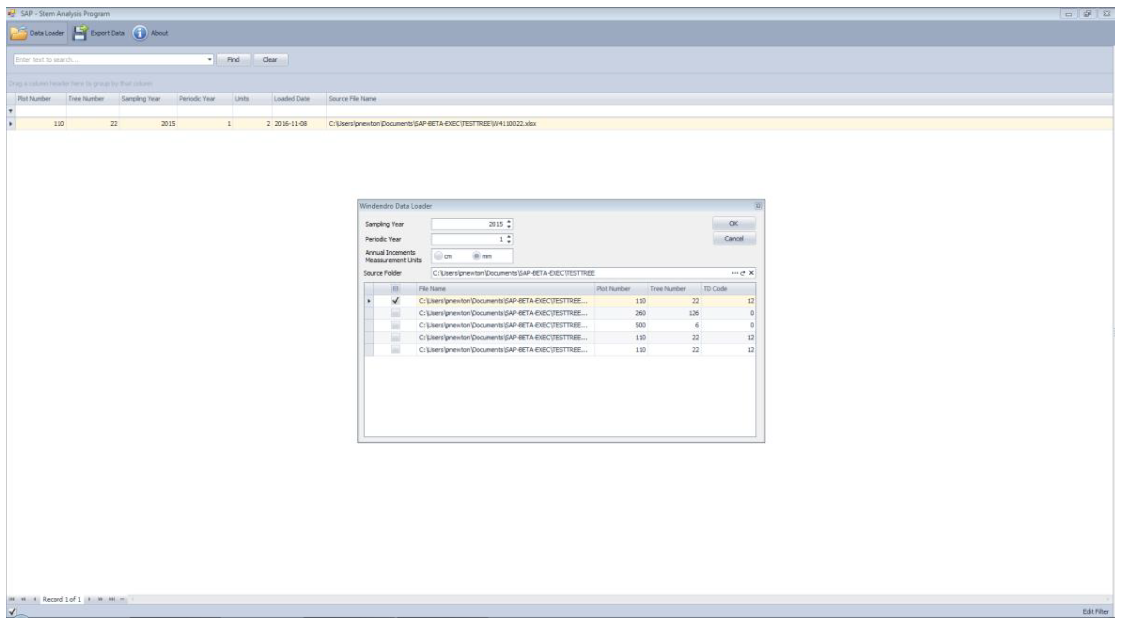
Figure 1. Screenshot of the “Data Loader” tool bar for the example tree.
Forests 10 01058 g001
Figure 2. Screenshot of the output data file/table list under the “Data” tool bar for the example tree, with the partial ST110022 file output displayed, which details the annual volumetric growth responses from 1984 to 2015 for the entire tree, inclusive of the 2nd thinning treatment in 1997 (n., the rapid increases in specific volume increment (TSVI) and relative growth rate (RGR) for approximately 7 years post-treatment (1997–2004)).
Forests 10 01058 g002
Figure 3. Screenshot of the output graphic list under the “Graphs” tool bar with the annual growth layer profiles displayed by year selected for the example tree.
Forests 10 01058 g003
Figure 4. Data verification for the 70 year-old jack pine example tree: illustration of the annual increment widths (mm) by year, radii (denoted R1 and R2 in legend) and cross-section. Note, the (1) section denotations (S: 1–11; y-axis) refer to the sections sampled at stump height, breast-height, and 10%, 20%, 30%, 40%, 50%, 60%, 70%, 80% and 90% relative height positions, respectively, (2) mean trend line for each cross-section is superimposed, and (3) thinning treatments occurred in years 1962 and 1997.
Forests 10 01058 g004
Figure 5. Entire growth layer profile for a 70 year-old jack pine tree.
Forests 10 01058 g005
Figure 6. Selected growth layer profiles for the example tree illustrating the longitudinal distribution of radial annual increment widths with increasing stem height, for the three years prior to the 1st and 2nd thinnings (1959–1961 and 1994–1996, respectively), the year of thinning treatments (1962 and 1997), the following three years after the 1st and 2nd thinnings (1963–1965 and 1998–2000, respectively).
Forests 10 01058 g006
Figure 7. Specific volume increment profile derived from a 70 year-old jack pine tree illustrating the distribution of relative responses throughout the stem for the 3 years prior to the 1st and 2nd thinnings (1959–1961 and 1994–1996, respectively), the year of thinning treatments (1962 and 1997), the following 3 years after the 1st and 2nd thinnings (1963–1965 and 1998–2000, respectively), and the final 3 years (2013–2015).
Forests 10 01058 g007
Figure 8. Relational temporal specific volume increment profiles derived from a 70 year-old jack pine tree, illustrating the distribution of relative response throughout the stem for each of the 18 years following the second (last) thinning (1998–2015; see legend).
Forests 10 01058 g008
Figure 9. Temporal specific volume increment profiles derived from a 70 year-old jack pine tree illustrating the distribution of relative response throughout the stem for each of the 18 years following the second (last) thinning (1998–2015).
Forests 10 01058 g009