Topography Affects Tree Species Distribution and Biomass Variation in a Warm Temperate, Secondary Forest

1
State Key Laboratory of Vegetation and Environment Change, Institute of Botany, Chinese Academy of Sciences, Beijing 100093, China
2
School of Natural Resources, University of Missouri, Columbia, MO 65211, USA
3
Key Laboratory of Ecological Restoration in Hilly Area, Pingdingshan University, Pingdingshan 467000, China
*
Author to whom correspondence should be addressed.
†
S.W. and G.Q. contributed equally to this work.
Forests 2019, 10(10), 895; https://doi.org/10.3390/f10100895
Submission received: 29 August 2019
/
Revised: 7 October 2019
/
Accepted: 7 October 2019
/
Published: 10 October 2019
(This article belongs to the Section Forest Ecology and Management)
Abstract
:A thorough understanding of carbon storage patterns in forest ecosystems is crucial for forest management to slow the rate of climate change. Here, we explored fine-scale biomass spatial patterns in a secondary warm temperate deciduous broad-leaved forest in north China. A 20-ha plot was established and classified by topographic features into ridge, valley, gentle slope, and steep slope habitats. Total tree biomass varied from 103.8 Mg/ha on the gentle slope habitats to 117.4 Mg/ha on the ridge habitats, with an average biomass of 109.6 Mg/ha across the entire plot. A few species produced the majority of the biomass, with five species contributing 78.4% of the total tree biomass. These five species included Quercus mongolica Fisch. ex Ledeb (41.7 Mg/ha, 38.1%), Betula dahurica Pall. (19.8 Mg/ha, 18.0%), Acer mono Maxim. (12.6 Mg/ha, 11.5%), Betula platyphylla Suk. (7.0 Mg/ha, 6.4%), and Populus davidiana Dode. (4.8 Mg/ha, 4.4%). The five species were also associated with certain habitats; for example, Q. mongolica was positively associated with the ridge habitat and A. mono was positively associated with the valley habitat. Results from this work document the variability in forest biomass across a warm temperate forest ecosystem of north China, with implications for managing and accounting forest carbon.
1. Introduction
Forests play a critical role in the Earth’s carbon cycle, providing a major carbon reservoir and serving as a globally important carbon sink [1,2,3]. Most of the total carbon pool within forest ecosystems is stored as either plant biomass or soil organic matter (SOM). Carbon stored within the SOM pool is relatively stable [4], whereas plant biomass carbon dynamics are closely related to patterns of ecological disturbance and forest stand dynamics that directly affect rates of carbon sequestration or release [5]. Losses in forest carbon have long been associated with land-use change and deforestation practices [6,7,8], and recent studies have attributed global patterns in carbon sinks to the regrowth of forest biomass following past disturbance through either afforestation of non-forest land or forest development following management [9,10].
Within forested landscapes, the distribution of carbon stored in plant biomass and the rate of carbon sequestration can be variable at local scales, with potential impacts on management or land use decisions [11]. Local forest carbon dynamics are related to abiotic drivers of productivity such as soil type, topographic position, aspect, and elevation, as well as biotic factors such as species composition and forest diversity [12,13,14]. Generally, site factors such as topographic position, aspect, and terrain shape affect availability of resources such as nutrients and water to drive forest productivity and biomass accumulation [15]. Similarly, site factors can also affect local tree composition, further accentuating differences in forest biomass through species-level variability in carbon storage within forests [16].
Forest biomass estimates are often based on inventory data from relatively small sample plots dispersed throughout a landscape [17,18,19]. These studies provide valuable estimation of carbon at broad spatial scales and often depict patterns of variation associated with regional site productivity [20,21]. However, these estimates are limited in that they represent average biomass values across representative forest conditions and are unable to capture fine-scale variability in biomass patterns within local environments [11,22].
A few large-scale forest plot studies have documented within-site biomass variation to improve the resolution at which carbon dynamics can be described [12,13,23,24]. For example, a 24-ha forest dynamics plot in Gutian Mountain, Zhejiang, China was used to describe biomass variation across topographic features [13]. The average aboveground biomass was 223.0 Mg/ha but varied among four topographically defined habitats, with the greatest biomass on lower ridge habitats and the least amount of biomass on upper ridge habitats. Differences in biomass among habitats were related, in part, to different habitat preferences and ecological strategies among tree species [13].
Previous studies reporting on large forest dynamics plots have mostly been from subtropical and tropical forests. Fine-scale relationships between biomass and environmental factors remains extremely limited in temperate forests, despite estimates that temperate forests stored 119 Pg C (14%) and contributed 27% and 34% to the global C sinks for 1990–1999 and 2000–2007, respectively [2]. In this study, we report on biomass patterns across topographic conditions from a 20-ha forest plot located in a temperate forest in China. The objectives of this study were to determine within-site biomass variability and biomass differences in tree species among forest habitats in a warm temperate forest ecosystem. The study makes it possible to evaluate fine-scale relationships between biomass and environmental factors in the temperate forest ecosystem.
2. Materials and Methods
2.1. Study Site and Data Collection
Xiaolongmen National Forest Park (115°26’ E, 39°58’ N) is located at the foot of Dongling Mountain in Beijing, China (Figure 1). The region is characterized by warm temperate deciduous broad-leaved forests, dominated by oak (Quercus mongolica) and maple (Acer mono). The study area has a temperate continental monsoon climate with a mean annual temperature of 4.3 °C and an annual precipitation of 589 mm [25]. The area is distributed with mountainous dark brown soil. Except for cliffs and ridges, the soil layer is generally above 30 cm, the surface litter layer is thick, the humus is well developed, and the soil is rich in organic matter. The region has a history of steel and iron production through the late 1950s, resulting in areas of secondary or planted forests that are generally 60 to 80 years old [26]. Selection harvesting during this period left some residual trees, with the largest oak trees about 100 years old. Since the 1950s, the region has been protected by the government in order to prevent water and soil loss and conserve biodiversity [27]. The study area was selected as representative of secondary forest in warm, temperate deciduous broad-leaved forest within the middle stages of succession in this region, and with generally similar land use history throughout [28,29].
In 2010, a 20-ha (400 × 500 m) permanent forest dynamics plot (DLS) was established in the core area of Xiaolongmen National Forest Park as part of the Chinese Forest Biodiversity Monitoring Network (CForBio; http://www.cfbiodiv.org/). All trees ≥1 cm diameter at breast height (1.3 m; DBH) were mapped, tagged, and identified to species following standard field procedures [30]. In total, we measured 52,681 trees across the entire plot, belonging to 51 species in 32 genera and 19 families. The most common species in the plot were Q. mongolica, A. mono, Betula dahurica, Syringa pubescens, Abelia biflora, and Corylus mandshurica.
2.2. Habitat Classification
The study area was divided into a 20 × 20 m grid (500 cells). For each cell, we calculated values for four topographical attributes: elevation, convexity, slope, and aspect. These four topographic attributes were computed for each 20 × 20 m cell in this study area based on protocols described by Lai, et al. [31] and Legendre, et al. [32]. Elevation for each cell was calculated as the average of the elevation of each cell vertex. Convexity was calculated as the elevation of the target cell minus the mean elevation of the eight surrounding cells. To determine slope and aspect, four triangular planes were created for each cell by connecting three of its corners. Slope was the deviation from horizontal for the mean of the four triangular planes, and aspect was calculated as the direction the slope faces. The negative cosine transformation of the aspect was used to be consistent with light intensity. The topographical information from each grid cell was used for habitat categorization using the Ward’s D hierarchical cluster analysis, which was computed with the “hclust” [33].
2.3. Forest Characteristics
Forest structure was described based on quadratic mean diameter (QMD), basal area, tree density, species richness, and biomass. The basal area was calculated as the sum of the cross-sectional areas of each stem at breast height and secondary stems at breast height that branched from the main stem below breast height. Total tree biomass was defined as the dry mass (Mg/ha) of all living trees with DBH ≥ 1 cm and was estimated using allometric equations (Table A1). For individuals with multiple stems, we summed the calculated biomass of each stem. Tree heights required for the allometric equations were estimated following the method described by Fang, et al. [34]. We used univariate analysis of variance (ANOVA) to determine effects of habitat (as identified through the cluster analysis) on each of the forest characteristics. Most values are reported as means ±95% confidence intervals (CI). To estimate 95% confidence intervals, 1000 bootstrap replicates for each 20 × 20 m subplot were generated.
2.4. Relative Contributions of Species to Total Biomass in Different Habitats
For each of the habitats identified through the cluster analysis, we determined the 10 tree species with the greatest biomass in each habitat and the entire plot. A modification of the torus-translation randomization test [35] was used to test whether a given species significantly contributed to the biomass of one or more habitat types. The 1999 translated maps were produced to provide a value of expected relative contribution. The observed relative contribution of a species was compared to the frequency distribution of expected values. If the observed value was ≤2.5% or ≥97.5% of the expected values, it was considered to have a significantly lower or higher contribution, respectively, to the habitat at a significance level of 0.05.
The relationships between biomass and environment (elevation, convexity, slope, aspect) and forest structure (quadratic mean diameter, basal area, tree density and species richness) were analyzed using spatial simultaneous autoregressive models at the cell level using the ‘spatialreg’ package. Models were run for the entire plot and for each habitat type, with the lowest AIC value indicating the best model fit. We calculated model efficiency (EF) following McEwan et al. [12], with EF = 1 indicating a 1-to-1 fit and values further from 1 indicating decreasing fit. All analyses were carried out using R version 2.12.
3. Results
3.1. Habitat Types
The DLS was spatially heterogeneous; elevation, convexity, slope, and aspect were 1394 m (range: 1292.2–1506.3 m), 0.03 m (−7.5–4.4 m), 32.0° (8.5°–48.5°), and 105.9° (0.1°–358.9°), respectively. The DLS was categorized into four habitats: ridge, valley, steep slope, and gentle slope (Figure 2 and Table 1). The valley habitat type was the largest (6.76 ha, 33.8% of the total area), and the steep slope habitat type was the smallest (3.48 ha, 17.4% of the total area).
3.2. Forest Characteristics across Habitat Types
Biomass averaged 109.6 Mg/ha (95% CI: 107.0–112.3 Mg/ha; Table 1) across the entire plot, and a total of 13 species made up the 10 highest biomass species for all habitat types. Jointly, these species contributed more than 95.0% of the total biomass in the plot (Table 2).
The five most common species contributed 78.4% of the total biomass, and the 10 most dominant tree species accounted for 91.1% of the total tree biomass. These five most important species were Quercus mongolica (41.7 Mg/ha, 38.1%), Betula dahurica (19.8 Mg/ha, 18.0%), Acer mono (12.6 Mg/ha, 11.5%), B. platyphylla (7.0 Mg/ha, 6.4%), and Populus davidiana (4.8 Mg/ha, 4.4%). In general, Q. mongolica had the largest mean QMD except for on the gentle slopes, and A. mono was the most abundant across habitat types (Table 3).
Forest structure significantly differed among these four habitat types (Table 1). The gentle slope had the lowest basal area (21.4 m2/ha, 95% CI: 20.3–22.6 m2/ha) and the lowest biomass (103.8 Mg/ha, 95% CI: 97.9–109.5 Mg/ha), whereas the ridge had the greatest basal area (25.8 m2/ha, 95% CI: 24.7–26.9 m2/ha), the lowest richness (10.3, 95% CI: 9.7–10.9), and the greatest biomass (117.4 Mg/ha, 95% CI: 112.1–122.9 Mg/ha). Basal area, richness, and biomass significantly differed between the gentle slope and the ridge. The steep slope had the greatest tree density (5965 trees/ha, 95% CI: 5426–6698 trees/ha).
3.3. Habitat-Specific Differentiation in Biomass Contribution
Of the 52 torus-translation tests, we found 19 significant associations of species with habitat types. Ten of the 13 most dominant tree species showed significant associations with one or several of the four habitat types (Table 2), with only Syringa pubescens, Ulmus macrocarpa and U. pumila not significantly associated with any habitat type. Steep slopes were positively associated with Fraxinus rhynchophylla and Tilia mongolica, and gentle slopes were positively associated with Beula dahurica, B. platyphylla, Sorbus discolor, and U. laciniata. The valley habitats were positively associated with Acer mono, Populus davidiana, and U. laciniata, whereas the ridge habitats were positively associated with Quercus mongolica.
No environmental variables were consistent significant predictors across the different habitat types. Although aspect was significant on steep slopes and slope was significant on gentle slopes, AIC indicated these were not the best predictors and EF < 0 for both relationships. Based on the AIC values, basal area was the best predictor of biomass across all habitat types and the entire plot (Table 4). According to EF, the fit was strongest on gentle slopes (EF = 0.76), steep slope (EF = 0.67), and ridge (EF = 0.59) but poor on valley habitats and across the entire plot (EF < 0).
4. Discussion
The biomass estimates from this study are consistent with previously published reports, with global patterns of forest biomass generally increasing from temperate to tropical regions [12,36]. Aboveground biomass estimates in some tropical forests may exceed 400 Mg/ha, whereas aboveground biomass in temperate regions have commonly been reported < 200 Mg/ha [12,37]. In China, studies have reported total tree biomass estimates up to nearly 300 Mg/ha in temperate regions (Figure 3). Reports of the greatest biomass in this region have been from broad-leaved Korean pine forests [38,39], although reports from oak forests have ranged widely (Figure 3). Biomass in birch and oak forests at Dongling Moutain ranged from 91.6–100 Mg/ha to 70–75.4 Mg/ha between 1992 and 1994 [34], and Sang, et al. [40] reported biomass of a warm temperate deciduous broad-leaved forest at 122.24 Mg/ha. While considerable variability has been reported for biomass values within temperate forests of China (Figure 3), studies have also documented the associated between forest age and biomass. For example, at Xiaoxing’an Mountains, oak forest biomass increased with increasing stand age, with 11.5 Mg/ha biomass at 24 age and 137.8 Mg/ha biomass at 101 age [41]. Results from our study fall near the middle of the biomass range for many of the reported studies, although we anticipate that biomass will increase as the forest continues to age.
Comprehensive understanding of carbon dynamics within forest systems requires information at several spatial scales. Information at broad spatial scales is necessary for generating national or global carbon budgets. Previous studies have noted that challenges with accurate forest carbon or biomass accounting have been improved by using consistent and robust field surveys of forest conditions [18,42,43]. However, the sampling protocols on national scales, such as the Forest Inventory and Analysis program in the United States, often sample at a plot intensity of one per > 1000 ha of land, a scale that cannot describe local variability in biomass stocks. Recent efforts to integrate remote sensing data with field inventory data show promise for improving the accuracy of broad-scale biomass and carbon estimates but are challenged to capture fine-scale variability missed by the field inventory [44,45]. The fine-scale sampling across the 20-ha plot in our study provides valuable information that is not available through from plot-based forest inventories. For example, the results demonstrate variability and patterns across different spatial scales, with examples of high local variability in forest biomass among adjacent grid cells (the 20 × 20 m scale) as well as broader patterns throughout the plot (e.g., relatively low biomass within the northeastern corner). Previous work from the study area estimated 122 Mg/ha biomass for this forest type based on forest inventory plots [40], suggesting that the overestimation of biomass was related, in part, to coarse sampling across local variability and habitat types.
Biomass varied substantially among the four habitats in our study, with the ridge sites supporting the greatest biomass and the gentle slope positions having the least. The four habitat types differed in topographic features, with ridge sites noted at the highest elevations and with the greatest convexity. In contrast, the valley habitats had the lowest convexity. Due to the rugged, incised character of the landscape, the ridge and valley habitats were not flat positions, although their slopes were intermediate between gentle and steep slope habitats. In addition, aspect was not found to strongly drive the habitat types, as none of the habitat types was identified as strongly associated with a single aspect. Topographic features, including those used to classify the habitats in this study, have commonly been associated with forest productivity. Terrain shape, aspect, and slope are commonly important drivers of nutrient and water availability [52,53,54]. In temperate forests of North America, productivity was found to decrease from cove to ridge positions and from low to high elevations, both of which associate with nutrient and water availability [15], and in the Shaanxi Province of interior China productivity generally decreased with elevation across the range observed in our study [55].
In addition to site productivity, forest biomass is also associated with interactions with disturbance patterns across topographical conditions. For example, in a subtropical forest in Taiwan, high aboveground biomass was found in flat areas that were protected from landslides caused by heavy rains during typhoons [12]. Despite greater soil productivity, lower stand biomass was also reported for low slope positions due to higher mortality from treefall during wet conditions in tropical rainforests of the Amazon basin [56]. In our study area, the history of anthropogenic disturbance, with selective harvesting for the developing iron and steel industries in the late 1950s, likely contributes to the patterns of forest biomass. For example, the greatest forest biomass was located on the ridge habitats, where trees were likely retained during the cutting period to block wind and stabilize soil on the ridge, although documentation of such patterns do not exist.
Legacy effects of past land use likely contribute to the successional development across the study area, with forest biomass previously reported to increase with stand age. For example, at Bingla Mountain, the oak forest biomass increased from 112 Mg/ha to 276 Mg/ha as forest age from 20 to 55 years old [48]. The forest of our study was generally 60 years old, although variation in stand age exists across the study area. Forest structural characteristics suggest that the ridge habitats may include older trees, in that the stands had relatively large QMD, basal area, and tree numbers. In contrast, the high tree number and lower QMD on steep slopes suggest these stands have abundant, small trees, often characteristic of early stages of stand development [57]. The strong relationship observed between stand basal area and biomass was expected because tree diameter is used to calculate both variables.
Similar to many previous studies (e.g., [13,58,59]), our results indicate that only a few species contributed to most of the tree biomass within the study area. Although the plot had 51 species, only five species accounted for 78.4% of the biomass and only 10 species accounted for 91.1% of the biomass. Several previous studies have found positive relationships between biodiversity and productivity in temperate forests [14,60,61], although the relationship has not been consistent across studies [62,63]. In temperate forests ecosystems, tree diversity is affected by complex interactions of climate, disturbance/successional development, herbivory, and other biological constraints [64,65,66,67]. Patterns of species dominance change through successional development [68], and much of the study area was relatively young following recovery from past land use.
We observed several patterns in species association with habitat types, although we found a few species (Quercus mongolica, Acer mono, and Betula dahuric) to be dominant across all sites types. Previous work from our study area found that the most dominant species on the site exhibited fewer patterns of spatial aggregation than rare species [29]. Despite the widespread distribution of A. mono, in particular, across the plot [29], our results demonstrate stronger association with the valley habitats than the ridge habitats, likely due to the greater nutrient and water availability within protected, concave landscape positions. In contrast, Q. mongolica, which was identified as the dominant species in each habitat excluding the gentle slope, was positively associated with the ridge habitats, representing harsher conditions that commonly favor the ecology of oak species [69]. Several species showed positive association with the gentle slope habitat type, including Betula dahurica, B. platyphylla, Sorbus discolor, and Ulmus laciniata. This habitat type was characterized by higher elevation and relatively concave landscape position, suggesting more mesic conditions suitable for the silvics of these species.
In general, the patterns of species composition and forest structure suggest the study area is transitioning through forest succession. Across all habitat types, Q. mongolica is a dominant canopy species, with the greatest DBH and basal area contribution for each habitat type excluding the gentle slopes. In contrast, the midstory across the entire study area is dominated by A. mono, indicative of successional transition from early successional birch forest to more shade-tolerant, mesic species exemplified by maple [70,71,72]. Through time, it is unclear if patterns of species composition across habitat types will change as localized tree mortality provides canopy openings for regeneration [70] or if species associations with habitat types will become stronger due to constraints on regeneration processes.
Intensively measured research plots, such as in this study, have long been used to describe detailed patterns in forest ecosystems (e.g., [73,74,75]). These plots provide valuable fine-scale data on ecosystem processes, forest dynamics, and patterns of variability at local scales. Individually, the plots reflect the local conditions within which they occur, and interpretation or extrapolation may be constrained to those specific conditions. In our study, the forest dynamics plot is located within a representative temperate, broad-leaved forest of the region and has been protected for over 60 years [28,29]. However, as with any forested landscape, the conditions we observe are influenced by not only the physical conditions of the area but also the legacy of past land use, indicating the importance of understanding context for interpretation. Recent efforts to increase the number of forest dynamics plots and coordinate efforts across plot networks provide critical opportunity for linking biomass data across spatial scales [76].
5. Conclusions
By establishing a large (20-ha) forest dynamics plot, we report on fine-scale variability and patterns in forest biomass across habitat types and tree species. Traditional forest inventory approaches commonly used in regional or national accounts of forest carbon sample at intensities at which one plot would represent our entire study area. Our results indicate important variability associated with habitat type, with tree biomass ranging from 103.8 Mg/ha on gentle slopes to 117.4 Mg/ha on ridge habitats. The mean biomass across the entire plot was 109.6 Mg/ha, falling within the range of biomass estimates reported for temperate ecosystems in China. Only a few tree species produced the majority of the biomass, with several of the species demonstrating association with specific habitat types. In general, the study area was dominated by Q. mongolica in the overstory and A. mono in the smaller diameter classes. Of the local topographic and stand characteristics measured in the study, forest biomass was most strongly, positively related to stand basal area and, to a lesser degree, to quadratic mean diameter. However, the weak relationships between topographic variables and biomass highlight the importance of composite descriptions of habitat types for estimating forest attributes such as biomass.
Our results provide information useful for both managing forest carbon and improving carbon accounting by providing baseline information on biomass for temperature forests of northern China. We expect that biomass will increase as the forest ages, although species composition may change through successional processes that vary across the habitat types. Understanding the fine-scale patterns in forest biomass and associated drivers, such as topographic features and species composition, can further improve accuracy of forest carbon estimates and be integrated with other data sources to scale up to broader estimates.
Author Contributions
S.W., G.Q. and B.O.K. designed and constructed this study framework; S.W. undertook data analysis and drafted the manuscript; B.O.K. contributed significantly to our introduction and discussion section.
Funding
This research was funded by National Key R&D Program of China (2017YFC0505601), National Natural Science Foundation of China (31570630 and 41601057) and State Key Laboratory of Forest and Soil Ecology (LFSE2015-13).
Acknowledgments
We are grateful to everyone involved in the data collection in the Dongling Moutain 20-ha plot.
Conflicts of Interest
The authors declare no conflict of interest.
Appendix A

Table A1.
Biomass allometric equations used in this study *.
| Species | Allometric Equations | Sources |
|---|---|---|
| Populus cathayana, Populus davidiana, Salix caprea, Salix phylicifolia, Salix viminalis | B = 0.085 × D2.48 | Wang et al. [77] |
| Corylus mandshurica | B = 0.148 × ((D2) × H)0.86 | Fang et al. [34] |
| Abelia biflora, Lonicera chrysantha, Lonicera hispida, Lonicera japonica, Sambucus williams, Viburnum sargentii | B = 0.00349 × ((D2) × H)1.04 | Fang et al. [34] |
| Deutzia grandiflora, Deutzia parviflora, Hydrangea bretschneideri, Philadelphus pekinensis, Ribes pulchellum | B = 0.014 × ((D2) × H)0.873 | Fang et al. [34] |
| Ulmus laciniata, Ulmus macrocarpa, Ulmus pumila | B = 0.07944 × ((D2) × H)0.9613 | Jiang [78] |
| Acer mono, Malus baccata, Prunus armeniaca, Prunus davidiana, Prunus padus, Sorbus discolor | B = 0.09747 × ((D2) × H)0.9510 | Jiang [78] |
| Quercus mongolica | B = 0.1122 × ((D2) × H)0.8500 | Jiang [78] |
| Juglans mandshurica | B = 0.11554 × ((D2) × H)0.8389 | Jiang [78] |
| Betula chinensis, Betula dahurica, Betula platyphylla | B = 0.16034 × ((D2) × H) 0.8354 | Jiang [78] |
| Fraxinus bungeana, Fraxinus rhynchophylla, Syringa pekinensis, Syringa pubescens | B = 0.19932 × ((D2) × H)0.8553 | Jiang [78] |
| Tilia mandshurica, Tilia mongolica | B = 0.20536 × ((D2) × H)0.7611 | Jiang [78] |
| Larix principis-rupprechtii | B = 0.01758 × ((D2) * H)0.9611 + 0.002 × ((D2) * H)1.1193 + 0.0038 × ((D2) * H)0.8828 + 0.01301 × ((D2) * H)0.8551 | Chen [79] |
| Lespedeza bicolor | B = 0.0202 × ((D2) × H)0.877 | Fang et al. [34] |
| Other species | B = 0.0481 × ((D2) × H)0.837 | Fang et al. [34] |
* B: dry biomass (kg), D: diameter at breast height (cm), H: tree height (m).
References
- Dixon, R.K.; Solomon, A.M.; Brown, S.; Houghton, R.A.; Trexier, M.C.; Wisniewski, J. Carbon pools and flux of global forest ecosystems. Science 1994, 263, 185–190. [Google Scholar] [CrossRef] [PubMed]
- Pan, Y.; Birdsey, R.A.; Fang, J.; Houghton, R.; Kauppi, P.E.; Kurz, W.A.; Phillips, O.L.; Shvidenko, A.; Lewis, S.L.; Canadell, J.G.; et al. A large and persistent carbon sink in the world’s forests. Science 2011, 333, 988–993. [Google Scholar] [CrossRef]
- Chen, L.; Guan, X.; Li, H.; Wang, Q.; Zhang, W.; Yang, Q.; Wang, S. Spatiotemporal patterns of carbon storage in forest ecosystems in Hunan Province, China. For. Ecol. Manag. 2019, 432, 656–666. [Google Scholar] [CrossRef]
- Davidson, E.A.; Janssens, I.A. Temperature sensitivity of soil carbon decomposition and feedbacks to climate change. Nature 2006, 440, 165–173. [Google Scholar] [CrossRef] [PubMed]
- Erb, K.-H.; Kastner, T.; Plutzar, C.; Bais, A.L.S.; Carvalhais, N.; Fetzel, T.; Gingrich, S.; Haberl, H.; Lauk, C.; Niedertscheider, M.; et al. Unexpectedly large impact of forest management and grazing on global vegetation biomass. Nature 2018, 553, 73–76. [Google Scholar] [CrossRef] [PubMed]
- Cramer, W.; Bondeau, A.; Schaphoff, S.; Lucht, W.; Smith, B.; Sitch, S. Tropical forests and the global carbon cycle: Impacts of atmospheric carbon dioxide, climate change and rate of deforestation. Philos. Trans. R. Soc. Lond. Ser. B Biol. Sci. 2004, 359, 331–343. [Google Scholar] [CrossRef]
- Van der Werf, G.R.; Morton, D.C.; DeFries, R.S.; Olivier, J.G.J.; Kasibhatla, P.S.; Jackson, R.B.; Collatz, G.J.; Randerson, J.T. CO2 emissions from forest loss. Nat. Geosci. 2009, 2, 737–738. [Google Scholar] [CrossRef]
- Woodwell, G.M.; Hobbie, J.E.; Houghton, R.A.; Melillo, J.M.; Moore, B.; Peterson, B.J.; Shaver, G.R. Global deforestation: Contribution to atmospheric carbon dioxide. Science 1983, 222, 1081–1086. [Google Scholar] [CrossRef] [PubMed]
- Erb, K.H.; Kastner, T.; Luyssaert, S.; Houghton, R.A.; Kuemmerle, T.; Olofsson, P.; Haberl, H. Bias in the attribution of forest carbon sinks. Nat. Clim. Chang. 2013, 3, 854–856. [Google Scholar] [CrossRef] [Green Version]
- Pugh, T.A.M.; Lindeskog, M.; Smith, B.; Poulter, B.; Arneth, A.; Haverd, V.; Calle, L. Role of forest regrowth in global carbon sink dynamics. Proc. Natl. Acad. Sci. USA 2019, 116, 4382–4387. [Google Scholar] [CrossRef] [Green Version]
- Houghton, R.A. Aboveground forest biomass and the global carbon balance. Glob. Chang. Biol. 2005, 11, 945–958. [Google Scholar] [CrossRef]
- McEwan, R.W.; Lin, Y.; Sun, I.F.; Hsieh, C.F.; Su, S.; Chang, L.; Song, G.; Wang, H.; Hwong, J.L.; Lin, K.; et al. Topographic and biotic regulation of aboveground carbon storage in subtropical broad-leaved forests of Taiwan. For. Ecol. Manag. 2011, 262, 1817–1825. [Google Scholar] [CrossRef]
- Lin, D.; Lai, J.; Muller-Landau, H.C.; Mi, X.; Ma, K. Topographic Variation in aboveground biomass in a subtropical evergreen broad-leaved forest in China. PLoS ONE 2012, 7, e48244. [Google Scholar] [CrossRef] [PubMed]
- Paquette, A.; Messier, C. The effect of biodiversity on tree productivity: From temperate to boreal forests. Glob. Ecol. Biogeogr. 2011, 20, 170–180. [Google Scholar] [CrossRef]
- Bolstad, P.V.; Vose, J.M.; McNulty, S.G. Forest productivity, leaf area, and terrain in Southern Appalachian deciduous forests. For. Sci. 2001, 47, 419–427. [Google Scholar]
- Kirby, K.R.; Potvin, C. Variation in carbon storage among tree species: Implications for the management of a small-scale carbon sink project. For. Ecol. Manag. 2007, 246, 208–221. [Google Scholar] [CrossRef]
- Fang, J.; Guo, Z.; Piao, S.; Chen, A. Terrestrial vegetation carbon sinks in China, 1981–2000. Sci. China Ser. D Earth Sci. 2007, 50, 1341–1350. [Google Scholar] [CrossRef]
- Botkin, D.B.; Simpson, L.G. Biomass of the North American boreal forest: A step toward accurate global measures. Biogeochemistry 1990, 9, 161–174. [Google Scholar]
- Goodale, C.L.; Apps, M.J.; Birdsey, R.A.; Field, C.B.; Heath, L.S.; Houghton, R.A.; Jenkins, J.C.; Kohlmaier, G.H.; Kurz, W.; Liu, S.; et al. Forest carbon sinks in the Northern hemisphere. Ecol. Appl. 2002, 12, 891–899. [Google Scholar] [CrossRef]
- Schroeder, P.; Brown, S.; Mo, J.; Birdsey, R.; Cieszewski, C. Biomass estimation for temperate broadleaf forests of the United States using inventory data. For. Sci. 1997, 43, 424–434. [Google Scholar]
- Fang, J.; Chen, A.; Peng, C.; Zhao, S.; Ci, L. Changes in forest biomass carbon storage in China between 1949 and 1998. Science 2001, 292, 2320–2322. [Google Scholar] [CrossRef] [PubMed]
- Su, Y.; Guo, Q.; Xue, B.; Hu, T.; Alvarez, O.; Tao, S.; Fang, J. Spatial distribution of forest aboveground biomass in China: Estimation through combination of spaceborne lidar, optical imagery, and forest inventory data. Remote Sens. Environ. 2016, 173, 187–199. [Google Scholar] [CrossRef] [Green Version]
- Valencia, R.; Foster, R.B.; Villa, G.; Condit, R.; Svenning, J.C.; Hernandez, C.; Romoleroux, K.; Losos, E.; Magard, E.; Balslev, H. Tree species distributions and local habitat variation in the Amazon: Large forest plot in eastern Ecuador. J. Ecol. 2004, 92, 214–229. [Google Scholar] [CrossRef]
- Chave, J.; Condit, R.; Lao, S.; Caspersen, J.P.; Foster, R.B.; Hubbell, S.P. Spatial and temporal variation of biomass in a tropical forest: Results from a large census plot in Panama. J. Ecol. 2003, 91, 240–252. [Google Scholar] [CrossRef]
- Su, H.; Li, G. Simulating the response of the Quercus mongolica forest ecosystem carbon budget to asymmetric warming. Chin. Sci. Bull. (Chin. Ver.) 2012, 57, 1544–1552. (In Chinese) [Google Scholar]
- Zou, Y.; Sang, W.; Wang, S.; Warrenthomas, E.; Liu, Y.; Yu, Z.; Wang, C.; Axmacher, J.C. Diversity patterns of ground beetles and understory vegetation in mature, secondary, and plantation forest regions of temperate northern China. Ecol. Evol. 2015, 5, 531–542. [Google Scholar] [CrossRef] [PubMed] [Green Version]
- Hou, J.; Mi, X.; Liu, C.; Ma, K. Tree competition and species coexistence in a Quercus-Betula forest in the Dongling Mountains in northern China. Acta Oecol. 2006, 30, 117–125. [Google Scholar] [CrossRef]
- Liu, H.; Xue, D.; Sang, W. Species diffusion and niche differentiation of the warm temperate deciduous broad-leaved forest in its functional development process. Chin. Sci. Bull. (Chin. Ver.) 2014, 59, 2359–2366. [Google Scholar]
- Gu, H.; Li, J.; Qi, G.; Wang, S. Species spatial distributions in a warm-temperate deciduous broad-leaved forest in China. J. For. Res. 2019. [Google Scholar] [CrossRef]
- Condit, R. Tropical Forest Census Plots: Methods and Results from Barro Colorado Island, Panama and a Comparison with Other Plots; Springer: Berlin/Landes, Germany; Georgetown, TX, USA, 1998. [Google Scholar]
- Lai, J.; Mi, X.; Ren, H.; Ma, K. Species-habitat associations change in a subtropical forest of China. J. Veg. Sci. 2009, 20, 415–423. [Google Scholar] [CrossRef]
- Legendre, P.; Mi, X.; Ren, H.; Ma, K.; Yu, M.; Sun, I.-F.; He, F. Partitioning beta diversity in a subtropical broad-leaved forest of China. Ecology 2009, 90, 663–674. [Google Scholar] [CrossRef] [PubMed]
- Borcard, D.; Gillet, F.; Legendre, P. Numerical Ecology with R; Springer: New York, NY, USA, 2011. [Google Scholar]
- Fang, J.; Liu, G.; Zhu, B.; Wang, X.; Liu, S. Study on the carbon cycle of three temperate forest ecological system in Donglingshan in Beijing. Sci. China Ser. D Earth Sci. 2006, 36, 533–543. [Google Scholar]
- Harms, K.; Condit, R.; Hubbell, S.P.; Foster, R.B. Habitat associations of trees and shrubs in a 50-ha neotropical forest plot. J. Ecol. 2001, 89, 947–959. [Google Scholar] [CrossRef]
- Saatchi, S.; Harris, N.; Brown, S.; Lefsky, M.; Mitchard, E.T.A.; Salas, W.; Zutta, B.R.; Buermann, W.; Lewis, S.L.; Hagen, S.; et al. Benchmark map of forest carbon stocks in tropical regions across three continents. Proc. Natl. Acad. Sci. USA 2011, 108, 9899–9904. [Google Scholar] [CrossRef] [PubMed] [Green Version]
- Wilson, B.T.; Woodall, C.W.; Griffith, D.M. Imputing forest carbon stock estimates from inventory plots to a nationally continuous coverage. Carbon Balance Manag. 2013, 8, 1. [Google Scholar] [CrossRef] [PubMed]
- Xu, Z.; Li, X.; Dai, H.; Tan, Z.; Zhang, Y.; Guo, X.; Peng, Y.; Dai, L. Research on biological productivity of Korean pine broadleaf forest. In Changbai Mountain in Forest Ecosystem Research; Wang, Z., Ed.; Forestry Press: Beijing, China, 1985; pp. 33–48. [Google Scholar]
- Wang, B.; Yang, X. Comparison of biomass and species diversity of four typical zonal vegetations. J. Fujian Coll For. 2009, 29, 345–350. [Google Scholar]
- Sang, W.; Ma, K.; Chen, L. Primary study on carbon cycling in warm temperate deciduous broad-leaved forest. Acta Phytoecol. Sin. 2002, 26, 543–548. [Google Scholar]
- Hu, H.; Luo, B.; Wei, S.; Wei, S.; Sun, L.; Luo, S.; Ma, H. Biomass carbon density and carbon sequestration capacity in seven typical forest types of the Xiaoxing’an Mountains, China. Chin. J. Plant Ecol. 2015, 39, 140–158. [Google Scholar]
- Brown, S. Measuring carbon in forests: Current status and future challenges. Environ. Pollut. 2002, 116, 363–372. [Google Scholar] [CrossRef]
- Edwards, T.C.; Cutler, D.R.; Zimmermann, N.E.; Geiser, L.; Moisen, G.G. Effects of sample survey design on the accuracy of classification tree models in species distribution models. Ecol. Model. 2006, 199, 132–141. [Google Scholar] [CrossRef]
- Blackard, J.A.; Finco, M.V.; Helmer, E.H.; Holden, G.R.; Hoppus, M.L.; Jacobs, D.M.; Lister, A.J.; Moisen, G.G.; Nelson, M.D.; Riemann, R.; et al. Mapping U.S. forest biomass using nationwide forest inventory data and moderate resolution information. Remote Sens. Environ. 2008, 112, 1658–1677. [Google Scholar] [CrossRef]
- Guitet, S.; Hérault, B.; Molto, Q.; Brunaux, O.; Couteron, P. Spatial structure of above-ground biomass limits accuracy of carbon mapping in rainforest but large scale forest inventories can help to overcome. PLoS ONE 2015, 10, e0138456. [Google Scholar] [CrossRef] [PubMed]
- Zhang, Q.; Wang, C. Carbon density and distribution of six Chinese temperate forest. Sci. China Life Sci. 2010, 53, 831–840. [Google Scholar] [CrossRef] [PubMed]
- Xu, Z.; Li, W.; Liu, W.; Wu, X. Study on the biomass and productivity of Mongolian oak forests in northeast region of China. Chin. J. Eco-Agric. 2006, 14, 21–24. [Google Scholar]
- Huo, C.; You, W.; Zhang, H.; Yan, T.; Wei, W.; Zhao, G.; Guo, J.; Xing, Z. Biomass and net primary productivity of Quecus mongolica plantation in Binglashan Mountains in Liaoning Province. J. Liaoning For. Sci. Technol. 2011, 4, 4–6, 11. [Google Scholar]
- Wang, D.; Cai, W.; Li, D.; Feng, X.; Feng, T.; Li, Y. Study of biomass and production of the forest of Quercus mongolica in Wuling Mountain. Chin. J. Ecol. 1998, 17, 9–15. [Google Scholar]
- Liu, Y.; Wu, M.; Guo, Z.; Jiang, Y.; Liu, S. Biomass and net productivity of Quercus variabilis forest in Baotianman Natural Reserve. Chin. J. Appl. Ecol. 1998, 9, 569–574. [Google Scholar]
- Liu, Y.; Wu, M.; Guo, Z.; Jiang, Y.; Liu, S.; Wang, Z.; Liu, B.; Zhu, X. Studies on biomass and net production of Quercus acutidentata forest in Baotianman Nature Reserve. Acta Ecol. Sin. 2001, 21, 1450–1456. [Google Scholar]
- Iverson, L.R.; Dale, M.E.; Scott, C.T.; Prasad, A. A GIS-derived integrated moisture index to predict forest composition and productivity of Ohio forests (U.S.A.). Landsc. Ecol. 1997, 12, 331–348. [Google Scholar] [CrossRef]
- Western, A.W.; Grayson, R.B.; Blöschl, G.; Willgoose, G.R.; McMahon, T.A. Observed spatial organization of soil moisture and its relation to terrain indices. Water Resour. Res. 1999, 35, 797–810. [Google Scholar] [CrossRef] [Green Version]
- McNab, W.H. A topographic index to quantify the effect of mesoscale landform on site productivity. Can. J. For. Res. 1993, 23, 1100–1107. [Google Scholar] [CrossRef]
- Chen, X.; Chen, J.; An, S.; Ju, W. Effects of topography on simulated net primary productivity at landscape scale. J. Environ. Manag. 2007, 85, 585–596. [Google Scholar] [CrossRef]
- Ferry, B.; Morneau, F.; Bontemps, J.-D.; Blanc, L.; Freycon, V. Higher treefall rates on slopes and waterlogged soils result in lower stand biomass and productivity in a tropical rain forest. J. Ecol. 2010, 98, 106–116. [Google Scholar] [CrossRef]
- Oliver, C.D. Forest development in North America following major disturbances. For. Ecol. Manag. 1980, 3, 153–168. [Google Scholar] [CrossRef]
- Knapp, B.O.; Pallardy, S.G. Forty-eight years of forest succession: Tree species change across four forest types in Mid-Missouri. Forests 2018, 9, 633. [Google Scholar] [CrossRef]
- Chen, J.; Xu, J.; Jensen, R.; Kabrick, J. Changes in aboveground biomass following alternative harvesting in oak-hickory forests in the eastern USA. iForest-Biogeosci. For. 2015, 8, 652–660. [Google Scholar] [CrossRef] [Green Version]
- Morin, X.; Fahse, L.; Scherer-Lorenzen, M.; Bugmann, H. Tree species richness promotes productivity in temperate forests through strong complementarity between species. Ecol. Lett. 2011, 14, 1211–1219. [Google Scholar] [CrossRef]
- Vilà, M.; Vayreda, J.; Comas, L.; Ibáñez, J.J.; Mata, T.; Obón, B. Species richness and wood production: A positive association in Mediterranean forests. Ecol. Lett. 2007, 10, 241–250. [Google Scholar] [CrossRef]
- Fei, S.; Jo, I.; Guo, Q.; Wardle, D.A.; Fang, J.; Chen, A.; Oswalt, C.M.; Brockerhoff, E.G. Impacts of climate on the biodiversity-productivity relationship in natural forests. Nat. Commun. 2018, 9, 5436. [Google Scholar] [CrossRef]
- Szwagrzyk, J.; Gazda, A. Above-ground standing biomass and tree species diversity in natural stands of Central Europe. J. Veg. Sci. 2007, 18, 555–562. [Google Scholar] [CrossRef]
- Glenn-Lewin, D.C. Species diversity in North American temperate forests. Vegetatio 1977, 33, 153–162. [Google Scholar] [CrossRef]
- Armesto, J.J.; Mitchell, J.D.; Villagran, C. A comparison of spatial patterns of trees in some tropical and temperate Forests. Biotropica 1986, 18, 1–11. [Google Scholar] [CrossRef]
- Hille Ris Lambers, J.; Clark, J.S.; Beckage, B. Density-dependent mortality and the latitudinal gradient in species diversity. Nature 2002, 417, 732–735. [Google Scholar] [CrossRef] [PubMed]
- Johnson, D.J.; Beaulieu, W.T.; Bever, J.D.; Clay, K. Conspecific negative density dependence and forest diversity. Science 2012, 336, 904–907. [Google Scholar] [CrossRef]
- Parker, G.R.; Leopold, D.J.; Eichenberger, J.K. Tree dynamics in an old-growth, deciduous forest. For. Ecol. Manag. 1985, 11, 31–57. [Google Scholar] [CrossRef]
- Larsen, D.R.; Johnson, P.S. Linking the ecology of natural oak regeneration to silviculture. For. Ecol. Manag. 1998, 106, 1–7. [Google Scholar] [CrossRef]
- Nowacki, G.J.; Abrams, M.D. The demise of fire and “Mesophication” of forests in the Eastern United States. BioScience 2008, 58, 123–138. [Google Scholar] [CrossRef]
- Yan, Q.; Zhu, J.; Yu, L. Seed regeneration potential of canopy gaps at early formation stage in temperate secondary forests, Northeast China. PLoS ONE 2012, 7, e39502. [Google Scholar] [CrossRef]
- Suh, M.H.; Lee, D.K. Stand structure and regeneration of Quercus mongolica forests in Korea. For. Ecol. Manag. 1998, 106, 27–34. [Google Scholar] [CrossRef]
- Lieberman, D.; Lieberman, M.; Peralta, R.; Hartshorn, G.S. Mortality patterns and stand turnover rates in a wet tropical forest in Costa Rica. J. Ecol. 1985, 73, 915–924. [Google Scholar] [CrossRef]
- Platt, W.J.; Evans, G.W.; Rathbun, S.L. The population dynamics of a long-lived conifer (Pinus palustris). Am. Nat. 1988, 131, 491–525. [Google Scholar] [CrossRef]
- Condit, R.; Ashton, P.S.; Manokaran, N.; LaFrankie, J.V.; Hubbell, S.P.; Foster, R.B. Dynamics of the forest communities at Pasoh and Barro Colorado: Comparing two 50-ha plots. Philos. Trans. R. Soc. B 1999, 354, 1739–1748. [Google Scholar] [CrossRef]
- Andersonteixeira, K.J.; Davies, S.J.; Bennett, A.C.; Gonzalezakre, E.B.; Mullerlandau, H.C.; Wright, S.J.; Abu Salim, K.; Almeyda Zambrano, A.M.; Alonso, A.; Baltzer, J.L.; et al. CTFS-ForestGEO: A worldwide network monitoring forest in an era of global change. Glob. Chang. Biol. 2015, 21, 528–549. [Google Scholar] [CrossRef]
- Wang, N.; Wang, B.; Wang, R.; Cao, X.; Wang, W.; Chi, L. Biomass allocation patterns and allometric models of Populus davidiaa and Pinus Tabulaeformis Carr. in west Shanxi province. Bull. Soil Water Conserv. 2013, 33, 151–155. [Google Scholar]
- Jiang, H. The Research on Plant Ecology; Institute of Botany: Beijing, China, 1992. [Google Scholar]
- Chen, S. Analyzing Features of Leaf Area Index, Net Primary Productivity and Tree-Ring for Typical Forest Communities in Warm Temperate Zone; Institute of Botany: Beijing, China, 2007. [Google Scholar]
Figure 1.
Location and contour map of the 20-ha (400 × 500 m) Dongling Moutain temperate forest plot.
Figure 1.
Location and contour map of the 20-ha (400 × 500 m) Dongling Moutain temperate forest plot.
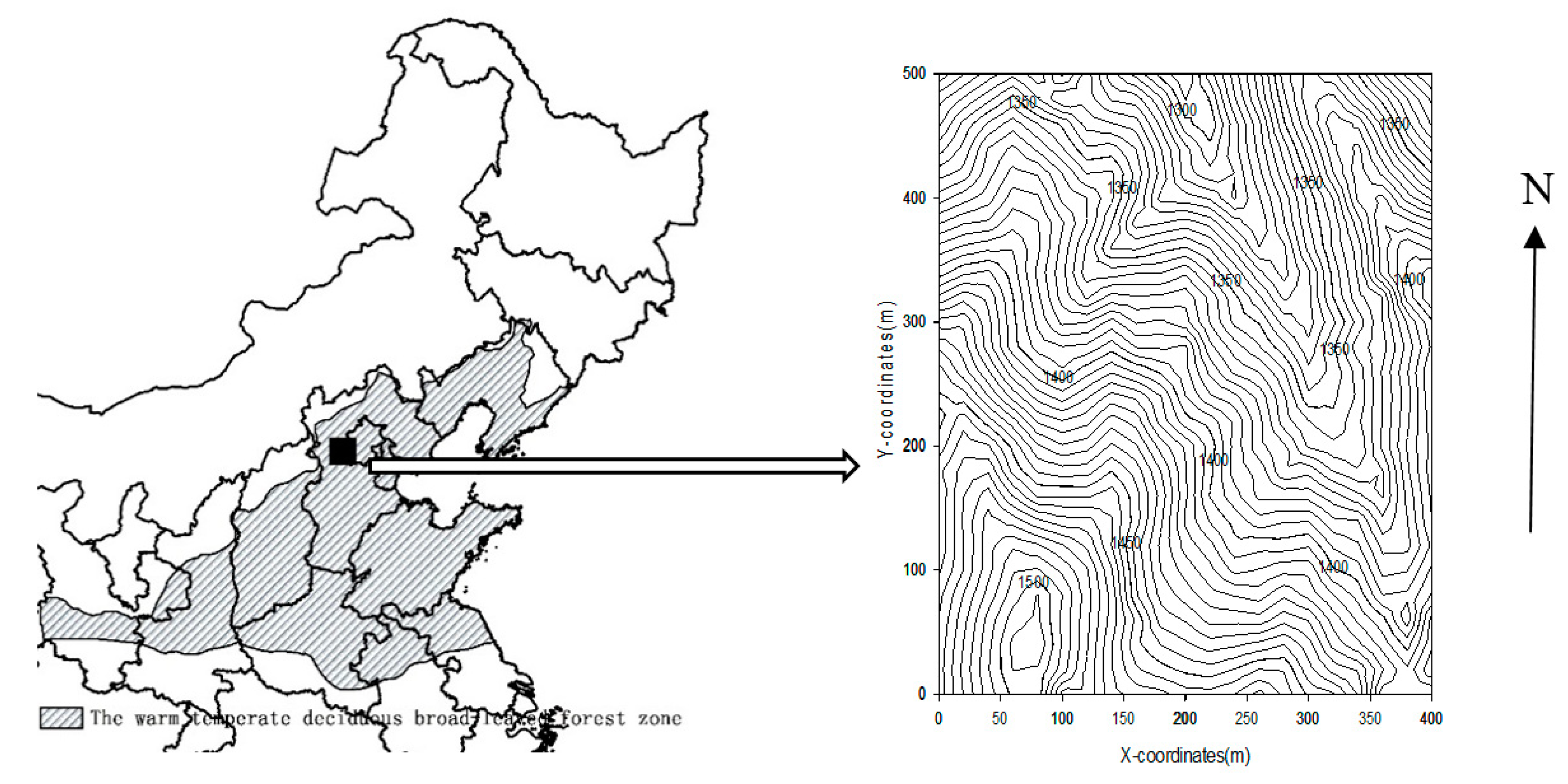
Figure 2.
Biomass (Mg/ha) for each grid cell, with habitat type identified through hierarchical cluster analysis (1: Steep slope; 2: Valley; 3: Ridge; 4: Gentle slope).
Figure 2.
Biomass (Mg/ha) for each grid cell, with habitat type identified through hierarchical cluster analysis (1: Steep slope; 2: Valley; 3: Ridge; 4: Gentle slope).
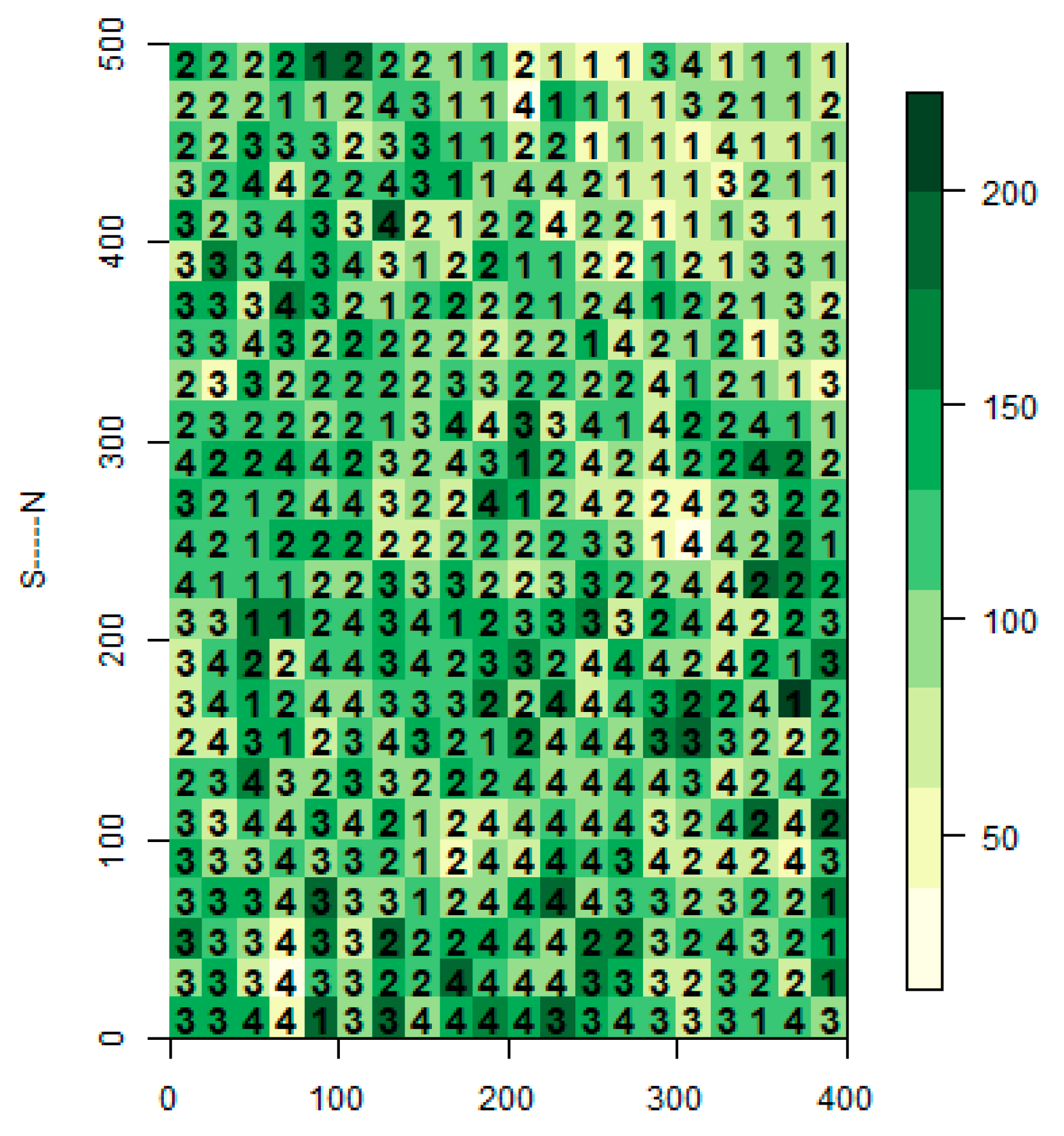
Figure 3.
Estimated biomass of the main temperate forests in China. The studies along the x-axis are organized from north to south as follows, X: Xiaoxing’an Mountains [41]; M: Maor Mountain [46]; L: Laoyeling Mountain [47]; C: Changbai Mountain [38,39]; B: Bingla Moutain [48]; W: Wuling Mountain [49]; D: Dongling Moutain ([34], this study); T: Baotianman [50,51].
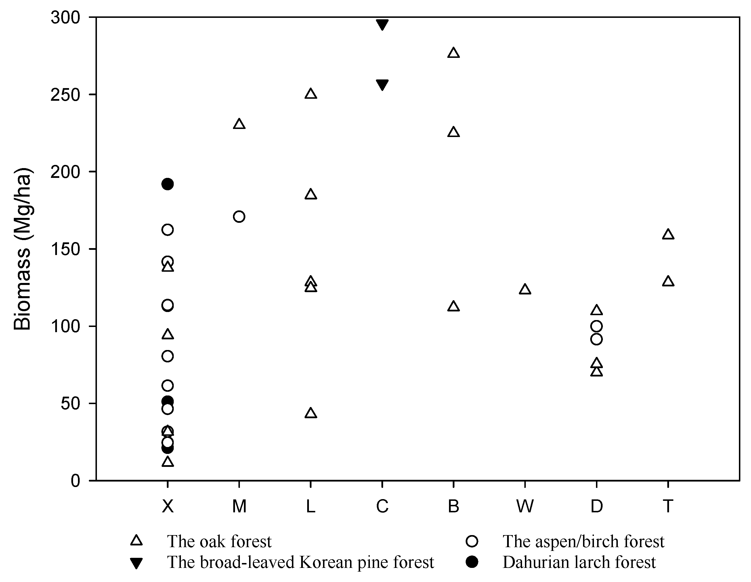
Table 1.
Topographical attribute (A) and forest structure (B) in four different habitats and the entire 20-ha DLS plot *.
Table 1.
Topographical attribute (A) and forest structure (B) in four different habitats and the entire 20-ha DLS plot *.
| (A) | |||||
| Habitat Category | Area (ha) | Elevation (m) | Convexity (m) | Slope (°) | Aspect (°) |
| Steep slope | 3.48 | 1367.73 (1359–1378) c | 0.05 (−0.29–0.42) b | 40.75 (40.24–41.40) a | 122.67 (103.6–143.6) a |
| Gentle slope | 4.6 | 1404.59 (1397–1414) b | −0.58 (−1.12–0.05) bc | 23.47 (22.62–24.10) d | 86.63 (77.95–97.76) b |
| Valley | 6.76 | 1381.87 (1376–1388) c | −0.87(−1.22–0.52) c | 34.21 (33.85–34.50) b | 104.97 (91.8–119.0) ab |
| Ridge | 5.16 | 1420.53 (1413–1429) a | 1.72 (1.46–2.06) a | 30.75 (30.39–31.12) c | 113.03 (100.1–129.7) ab |
| Entire plot | 20 | 1394.61 (1390–1399) | 0.03 (−0.18–0.26) | 31.98 (31.42–32.52) | 105.91 (98.9–113.5) |
| (B) | |||||
| Habitat Category | Quadratic Mean Diameter (cm) | Basal Area (m2/ha) | Tree Density (Trees/ha) | Richness (Number of Species/400 m2) | Biomass (Mg/ha) |
| Steep slope | 7.51 (7.08–8.07) b | 22.7(21.2–24.2) bc | 5965(5426–6698) a | 11.6(10.9–12.3) a | 104.8(98.5–111.7) b |
| Gentle slope | 8.27 (7.91–8.70) ab | 21.4(20.3–22.6) c | 4616(4195–5091) b | 11.7(11.1–12.3) a | 103.8(97.9–109.5) b |
| Valley | 8.52 (8.21–8.91) a | 23.4(22.6–24.3) b | 4875(4491–5279) b | 12.1(11.6–12.7) a | 109.9(105.8–114.3) ab |
| Ridge | 8.88 (8.32–9.53) a | 25.8(24.7–26.9) a | 5515(5011–6111) ab | 10.3(9.7–10.9) b | 117.4(112.1–122.9) a |
| Entire plot | 8.38 (8.18–8.60) | 23.4(22.9–24.0) | 5171(4904–5413) | 11.5(11.1–11.8) | 109.6(107.1–112.4) |
* Quadratic mean diameter, tree density, biomass and basal area were transformed by the quadratic equation in univariate analysis of variance (ANOVA). Values are means with bootstrapped 95% confidence intervals in parentheses. The different letter indicated the significant difference among columns.
Table 2.
Relative species’ contributions to biomass in the four different habitats and the entire 20-ha DLS plot based on torus-translation test *.
Table 2.
Relative species’ contributions to biomass in the four different habitats and the entire 20-ha DLS plot based on torus-translation test *.
| Species Code | Steep Slope | Gentle Slope | Valley | Ridge | Entire Plot |
|---|---|---|---|---|---|
| Acer mono | 14.19 (13.53%) | 10.59 (10.20%) | 15.93 (14.49%) + | 9.15 (7.80%) - | 12.65 (11.55%) |
| Betula dahurica | 11.56 (11.02%) - | 27.25 (26.25%) + | 16.43 (14.94%) | 22.95 (19.55%) | 19.75 (18.03%) |
| Betula platyphylla | 2.88 (2.75%) - | 11.08 (10.67%) + | 5.13 (4.66%) - | 8.53 (7.26%) | 6.98 (6.37%) |
| Fraxinus rhynchophylla | 7.27 (6.94%) + | 1.06 (1.02%) | 1.57 (1.43%) | 1.70 (1.45%) | 2.48 (2.26%) |
| Juglans mandshurica | 3.57 (3.41%) | 6.61 (6.36%) | 5.33 (4.85%) | 0.89 (0.76%)- | 4.17 (3.81%) |
| Populus davidiana | 2.27 (2.16%) | 5.95 (5.73%) | 6.69 (6.08%) + | 3.00 (2.55%) | 4.80 (4.38%) |
| Quercus mongolica | 43.80 (41.78%) | 23.47 (22.61%) - | 40.34 (36.70%) | 58.41 (49.74%) + | 41.72 (38.08%) |
| Sorbus discolor | 0.97 (0.92%) - | 4.52 (4.35%) + | 2.68 (2.44%) | 1.50 (1.28%) | 2.50 (2.28%) |
| Syringa pubescens | 2.69 (2.56%) | 1.70 (1.63%) | 2.63 (2.39%) | 2.72 (2.32%) | 2.45 (2.24%) |
| Tilia mongolica | 3.39 (3.24%) + | 0.71 (0.68%) | 1.59 (1.45%) | 0.82 (0.70%) - | 1.51 (1.37%) |
| Ulmus laciniata | 1.05 (1.00%) | 2.55 (2.46%) + | 2.14 (1.95%) + | 0.01 (0.01%) - | 1.50 (1.37%) |
| Ulmus macrocarpa | 2.03 (1.94%) | 1.43 (1.37%) | 1.96 (1.78%) | 1.23 (1.04%) | 1.66 (1.51%) |
| Ulmus pumila | 3.38 (3.22%) | 1.93 (1.86%) | 1.74 (1.58%) | 2.59 (2.21%) | 2.29 (2.09%) |
* Numbers represented species biomass (Mg/ha), and the percent in parentheses represented percent of species biomass divided by habitat biomass. Based on the torus-translation tests, ‘+’ and ‘-’ indicated contributions that were significantly higher and lower at individual test significance levels of 0.05, respectively.
Table 3.
Quadratic mean diameter (A, cm), basal area (B, m2/ha) and density (C, trees/ha) of the five most common tree species in the four different habitats and the entire 20-ha DLS plot *.
Table 3.
Quadratic mean diameter (A, cm), basal area (B, m2/ha) and density (C, trees/ha) of the five most common tree species in the four different habitats and the entire 20-ha DLS plot *.
| (A) | |||||
| Species | Steep Slope | Gentle Slope | Valley | Ridge | Entire |
| Acer mono | 5.3 (4.83–5.72) ab | 5.56 (5.01–6.26) ab | 6.26 (5.82–6.81) a | 5.00 (4.53–5.63) b | 5.61 (5.37–5.91) |
| Betula dahurica | 7.72 (6.19–9.29) c | 16.12 (14.58–17.45) a | 12.61 (11.27–13.93) b | 13.97 (12.39–15.12) ab | 12.92 (12.22–13.66) |
| Betula platyphylla | 2.93 (1.91–4.32) c | 10.25 (8.47–12.14) a | 7.18 (5.97–8.92) b | 8.70 (7.15–10.24) ab | 7.54 (6.68–8.39) |
| Populus davidiana | 3.20 (2.23–4.36) c | 5.70 (4.36–7.25) ab | 6.46 (5.34–7.61) a | 3.57 (2.71–4.53) bc | 4.97 (4.36–5.62) |
| Quercus mongolica | 15.05 (13.51–16.26) ab | 9.59 (7.68–11.57) c | 14.75 (13.33–16.02) b | 17.98 (16.72–19.13) a | 14.45 (13.67–15.18) |
| (B) | |||||
| Species | Steep Slope | Gentle Slope | Valley | Ridge | Entire |
| Acer mono | 2.25 (1.85–2.80) ab | 1.58 (1.27–2.01) bc | 2.40 (2.13–2.79) a | 1.42 (1.18–1.71) c | 1.93 (1.77–2.11) |
| Betula dahurica | 2.28 (1.73–3.04) b | 5.05 (4.30–5.90) a | 3.09 (2.60–3.67) b | 4.32 (3.58–5.07) a | 3.72 (3.40–4.11) |
| Betula platyphylla | 0.55 (0.32–0.91) c | 2.05 (1.57–2.53) a | 0.96 (0.72–1.32) bc | 1.58 (1.18–2.06) ab | 1.30 (1.12–1.53) |
| Populus davidiana | 0.58 (0.32–0.93) b | 1.31 (0.91–1.78) ab | 1.55 (1.21–1.97) a | 0.73 (0.49–1.08) b | 1.11 (0.93–1.32) |
| Quercus mongolica | 10.32 (8.54–12.25) ab | 5.49 (4.08–7.32) c | 9.36 (7.95–11.00) b | 13.55 (11.81–15.41) a | 9.72 (8.87–10.57) |
| (C) | |||||
| Species | Steep Slope | Gentle Slope | Valley | Ridge | Entire |
| Acer mono | 864.08 (750.2–1014.0) a | 583.91 (504.2–682.0) b | 793.05 (716.4–893.0) a | 612.60 (539.0–713.9) b | 710.75 (660.2–762.3) |
| Betula dahurica | 218.68 (146.6–316.0) a | 186.52 (159.1–211.4) a | 151.78 (128.0–187.5) a | 199.81 (171.6–240.7) a | 183.8 (164.6–206.8) |
| Betula platyphylla | 39.94 (23.56–67.53) b | 82.17 (61.74–109.05) a | 42.90 (32.28–58.35) b | 62.60 (47.87–79.84) ab | 56.5 (48.05–66.00) |
| Populus davidiana | 76.44 (44.32–121.55) a | 82.83 (57.83–128.69) a | 111.98 (88.2–140.8) a | 81.98 (58.18–118.79) a | 91.35 (76.55–109.25) |
| Quercus mongolica | 525.86 (443.9–632.1) a | 206.52 (151.8–277.3) c | 342.31 (292.0–409.4) b | 515.31 (448.4–597.0) a | 387.65 (349.1–422.4) |
* Values were means with bootstrapped 95% confidence intervals in parentheses. The different letter indicated the significant difference among rows.
Table 4.
The relationships between biomass and environment and forest structure variables including elevation, convexity, slope, aspect, quadratic mean diameter, basal area, tree density, and species richness *.
Table 4.
The relationships between biomass and environment and forest structure variables including elevation, convexity, slope, aspect, quadratic mean diameter, basal area, tree density, and species richness *.
| Biomass (Mg/ha) | Steep Slope | Gentle Slope | Valley | Ridge | Entire Plot |
|---|---|---|---|---|---|
| Elevation (m) | −85.13~0.14 (4803.3) | ||||
| Convexity (m) | 148.32~2.15 (4802.5) | ||||
| Slope (°) | 87.68~2.6 (1108.2) | 115.73~1.10 (4788.4) | |||
| aspect (°) | 161.46~15.77 (833.7) | ||||
| Quadratic mean diameter (cm) | −0.22~5.05 (821.7) | 126.53~6.0 (1097.3) | 143.04~6.0 (1578.8) | 138.42~4.93 (1226.2) | 97.44~6.67 (4699.9) |
| Basal area (m2/ha) | −3.61~4.18 (698.8) | 14.51~4.34 (940.5) | 31.85~4.42 (1345.5) | 19.65~4.31 (1037.7) | 34.69~4.41 (3909.3) |
| Tree density (trees/ha) | 140.51~0.001 (4806.5) | ||||
| Species richness (number/400 m2) |
* Only significant slope values are shown (p < 0.05). The negative cosine transformation of the aspect was used in the linear regression. The number before wave line is intercept, the number after wave line is slope, and value in parentheses is AIC.
© 2019 by the authors. Licensee MDPI, Basel, Switzerland. This article is an open access article distributed under the terms and conditions of the Creative Commons Attribution (CC BY) license (http://creativecommons.org/licenses/by/4.0/).
Share and Cite
MDPI and ACS Style
Wang, S.; Qi, G.; Knapp, B.O. Topography Affects Tree Species Distribution and Biomass Variation in a Warm Temperate, Secondary Forest. Forests 2019, 10, 895. https://doi.org/10.3390/f10100895
AMA Style
Wang S, Qi G, Knapp BO. Topography Affects Tree Species Distribution and Biomass Variation in a Warm Temperate, Secondary Forest. Forests. 2019; 10(10):895. https://doi.org/10.3390/f10100895
Chicago/Turabian StyleWang, Shunzhong, Guang Qi, and Benjamin O. Knapp. 2019. "Topography Affects Tree Species Distribution and Biomass Variation in a Warm Temperate, Secondary Forest" Forests 10, no. 10: 895. https://doi.org/10.3390/f10100895
Note that from the first issue of 2016, this journal uses article numbers instead of page numbers. See further details here.