Article

Identifying Biases in Global Tree Cover Products: A Case Study in Costa Rica

University of Maryland, Baltimore County, Baltimore, MD 21250, USA
*
Author to whom correspondence should be addressed.
Forests 2019, 10(10), 853; https://doi.org/10.3390/f10100853
Submission received: 15 August 2019 / Revised: 5 September 2019 / Accepted: 27 September 2019 / Published: 30 September 2019
(This article belongs to the Section Forest Inventory, Modeling and Remote Sensing)

Abstract

:
Global tree cover products are widely used in analyses of deforestation, fragmentation, and connectivity, but are rarely critically assessed. Inaccuracies in these products could have consequences for future decision making, especially in data-poor regions like the tropics. In this study, potential biases in global and regional tree cover products were assessed across a diverse tropical country, Costa Rica. Two global tree cover products and one regional national forest cover map were evaluated along biophysical gradients in elevation, precipitation, and agricultural land cover. To quantify product accuracy and bias, freely available high-resolution imagery was used to validate tree and land cover across these gradients. Although the regional forest cover map was comparable in accuracy to a widely-used global forest map (the Global Forest Change of Hansen et al., also known as the GFC), another global forest map (derived from a cropland dataset) had the highest accuracy. Both global and regional forest cover products showed small to severe biases along biophysical gradients. Unlike the regional map, the global GFC map strongly underestimated tree cover (>10% difference) below 189 mm of precipitation and at elevations above 2000 m, with a larger bias for precipitation. All map products misclassified agricultural fields as forest, but the GFC product particularly misclassified row crops and perennial erect crops (banana, oil palm, and coffee), with maximum tree cover in agricultural fields of 89%–100% across all crops. Our analysis calls into further question the utility of the GFC product for global forest monitoring outside humid regions, indicating that, in tropical regions, the GFC product is most accurate in areas with high, aseasonal rainfall, low relief, and low cropland area. Given that forest product errors are spatially distributed along biophysical gradients, researchers should account for these spatial biases when attempting to analyze or generate forest map products.

Graphical Abstract

1. Introduction

Humid tropical forests play a vital role in various global processes and are under threat [1,2,3,4,5]. Accurate global and regional maps are needed to support conservation policies across the tropics [5,6,7,8], and recent advances in remote sensing have enabled global maps of tropical forest ecosystems [5,9,10]. However, accurately measuring forest cover in the humid tropics is difficult [11]. There are many challenges in estimating tropical forest cover at regional and global scales using remote sensing. Global maps of tree cover must account for variability along numerous abiotic and biotic gradients, including topography [12], high cloud cover [13,14], precipitation [15], phenological variability [16], and the widespread occurrence of perennial erect crops (“tree crops”) that can be confused with forest cover [17,18,19]. As a result, there are relatively few global tree cover products, and no global products that distinguish natural forest cover from agricultural tree cover. In this study, we examine whether current products under- or over-estimate tree cover along gradients of topography, precipitation, and agricultural cover.
Forest cover maps derived from passive optical imagery (e.g., Landsat) require cloud-free imagery for complete, wall-to-wall coverage [11]. Cloud cover is high and persistent over the humid tropics, often aseasonal, and is especially common at high elevation and over forested landscapes [13,20,21]. As a result, cloud-free days are rare, making it difficult to use satellite imagery for timely ground observations [14]. Extensive image compositing is often necessary to create cloud-free imagery over humid tropical forests, and the resulting composite images can still be contaminated with cloud and cloud shadow effects [22]. At higher elevations or in rough terrain, the combined effects of cloud compositing and topographical shadowing on reflectance estimates can make land cover classification particularly challenging [12].
Furthermore, when there are cloud-free days in the tropics, they often occur during the dry season, when the vegetation is not as green and/or is partially or completely drought-deciduous [14]. Phenological variability makes mapping tropical forest cover more challenging [23,24,25]. For example, remote sensing of canopy cover in tropical humid forests is more accurate than in tropical dry forests [26]. In tropical dry forests, many canopy tree species shed their leaves in the dry season. To accurately quantify tropical dry forest cover, wet season imagery is required [27], which is often contaminated with clouds [14]. However, even in humid tropical forests, which receive higher levels of precipitation, precipitation can vary over the year to create distinct wet and dry seasons [28,29]. Although humid forests maintain high leaf cover year-round, they undergo both seasonal variations in greenness and interspecific variability in leaf phenology [30]. In both wet and dry tropical forests, seasonal changes in precipitation drive shifts in vegetation spectral reflectance, which can lead to misclassification and underprediction of forest cover in the dry season.
Another major challenge in accurately measuring tropical forest cover is differentiating between natural forest cover and trees established for agriculture (“tree crops”). Tree crops such as oil palm, eucalyptus, banana, and rubber are increasingly common across the tropics [17,31]. Although FAO (Food and Agricultural Organization) statistics for tree plantation and tree crop area exist at the country scale, they are spatially aggregated estimates intended for calculating net national tree cover change [32]. Current global tree cover maps do not attempt to differentiate between tree crops and natural forest [5,10]. For example, the Global Forest Change dataset (GFC), a widely used forest cover map (3000+ citations), defines forest cover as all trees >5 m in height [5]. Tropek et al. [17] pointed out that the GFC forest cover map includes many types of non-forest tree cover, from timber plantations to perennial crops like banana and oil palm. Because tree crops do not provide the same ecosystem service and biodiversity benefits as natural forest cover [17,33,34], confusing tree crops with natural forest leads to inaccurate estimates of tropical biodiversity, forest loss, and forest recovery [35,36].
One potential solution to the challenges inherent in mapping global forest cover is to simply use regional maps of tree and forest cover, which are often assumed to be more accurate than global maps [37]. For example, UN-RED maps tracking forest cover change require national forest/non-forest classifications based on national forest definitions [38,39]. However regional maps of forest cover can face similar challenges across abiotic and biotic gradients [11,12,21]. Regional maps also take additional effort and money to create and validate, especially when global tree cover products already exist [40,41]. Using global tree cover products to inform or replace regional forest cover maps has been shown to improve forest cover estimates and the accuracy of forest inventories [41]. Furthermore, global percent tree cover maps permit direct comparisons of forest change between countries, as national forest cover estimates can vary widely given national forest definitions [39]. More direct comparisons of the accuracy of global and regional forest cover products are necessary to test the assumption of higher regional accuracy, especially across diverse abiotic and biotic gradients.
In this study, we quantified error and bias in regional and global forest cover products in Costa Rica, a tropical country in Central America. Error in tree cover estimates was defined as observable deviation of predicted tree cover from reference measurements; bias in tree cover estimates occurs where this deviation is predictable along, and correlated with, gradients of interest. Like many other countries in the tropics, Costa Rica has large gradients in precipitation and topography and a variety of tree crops, including oil palm and banana. Available forest cover products vary widely in their estimates of total forest cover in the country (from 50% to 60%). Across Costa Rica, we compared the performance of global and regional forest cover products and tested for the presence of systematic biases in forest cover estimates along gradients of precipitation, topography, and agricultural cover.

2. Materials and Methods
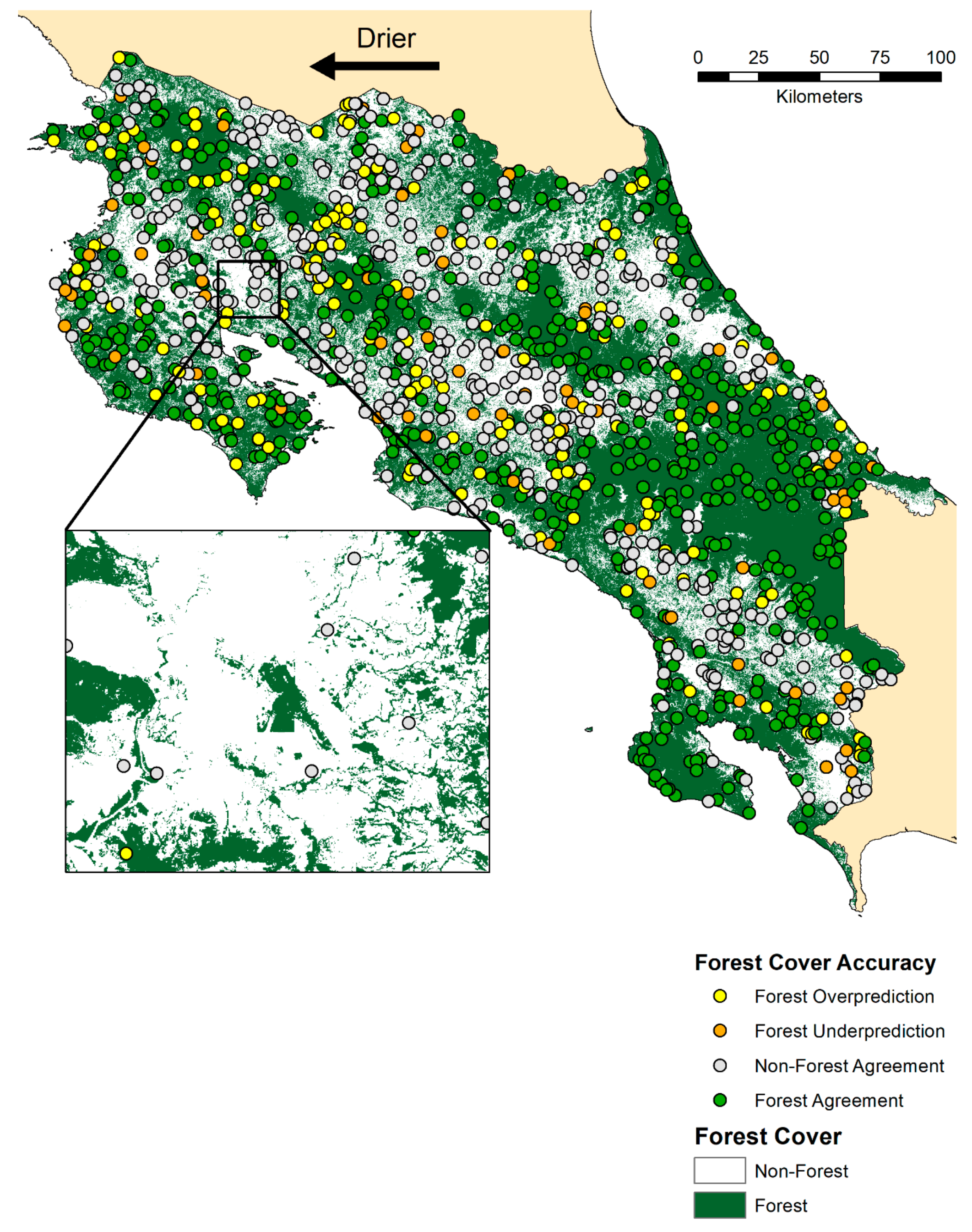
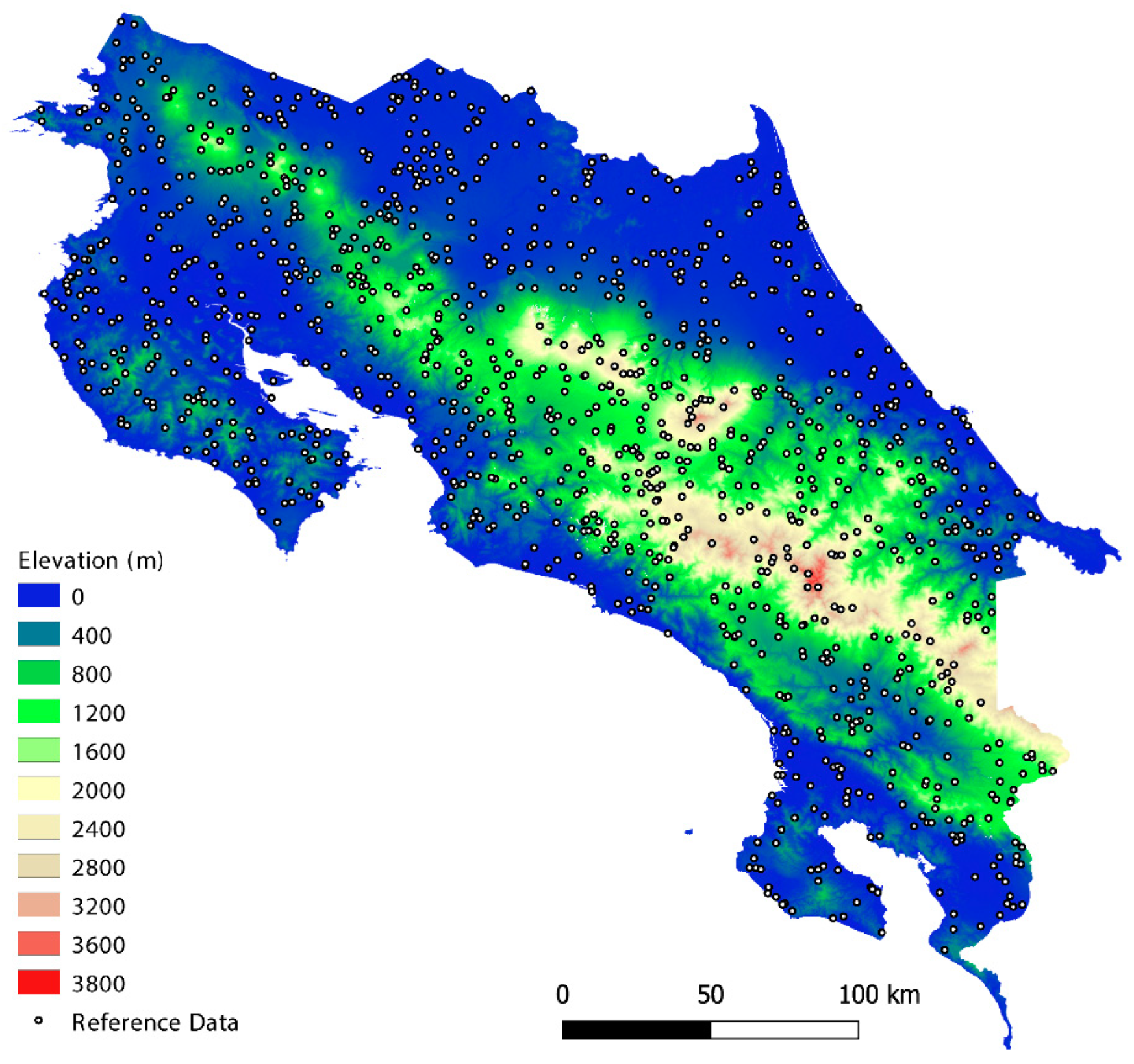
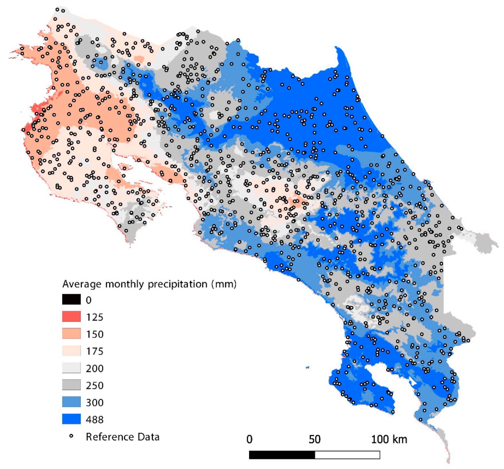
2.1. Study Area

Costa Rica is a small Central American country (~51,000 km2) located between Nicaragua and Panama [27,42]. Although Costa Rica represents only 0.03% of the Earth’s surface area, it contains about 6% of the world’s biodiversity [43]. The country has a diversity of tropical ecosystems, containing 12 different Holdridge life zones [44], which are defined by average annual values of temperature, precipitation, and altitude. Tropical dry forests and humid forests cover extensive areas in Costa Rica, and can be distinguished by their average monthly precipitation as well as seasonal phenology. Average monthly precipitation across Costa Rica ranges from about 70 mm to 410 mm [45] and elevation ranges from sea level to ~4000 m [8].

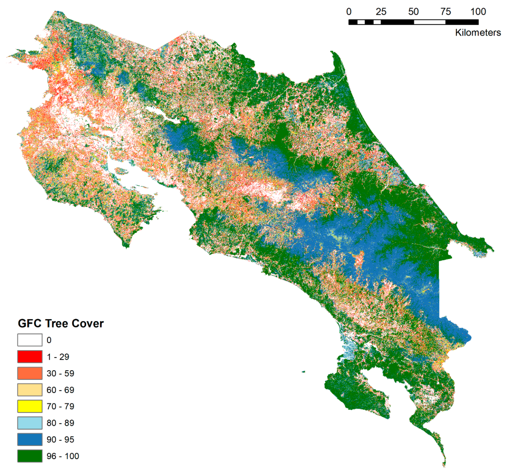
2.2. Tree Cover Products

We compared two global tree cover products and one regional tree cover product over Costa Rica (Table 1). The two global products were: (1) The University of Maryland’s Global Forest Change 2000–2015 tree canopy cover product (version 1.3) developed by Hansen et al. [5] (hereafter GFC, or Hansen; and (2) a modification of the Massey et al. [46,47] global cropland dataset (GCL). The regional product (hereafter, Landa) was developed specifically for Costa Rica by Fernandez-Landa et al. [8] using a Landsat imagery time series between 1985 and 2014.
The GFC product quantifies global tree cover (vegetation taller than 5 m) in the year 2000 and quantifies global forest change (tree cover gain and loss) between 2000 and 2015. To estimate tree cover circa 2015, we added the forest gain pixels (2000–2012) and subtracted the loss pixels (2000–2015) from the 2000 tree cover estimates (0%–100%). Gain pixels were given a tree cover value of 100% (seven reference pixels affected, see below) and loss pixels were given a tree cover value of 0% (42 reference pixels affected, see below).
The other global product used in this research was a modified 2010 global cropland (GCL) dataset [46]. The original GCL dataset consisted of three classes: cropland areas (crops and pastures), non-cropland areas (bare ground, urban areas, forest, etc.), and water. In post-classification processing, it was filtered to remove patches smaller than 0.18 hectares (i.e., two four-connected neighboring pixels). We modified the original GCL dataset to create a tree cover map in two steps. First, we eliminated agricultural areas and water by selecting the non-cropland classification category. We then eliminated non-forest areas from the GCL non-cropland category by removing pixels where the GFC product had 0% tree cover values (i.e., urban areas, bare ground, and other non-forest). This process created the derived GCL product, a forest/non-forest binary classification for the year 2010.
Like the derived GCL global product, the regional Landa product is a forest/non-forest binary classification, for the year 2014. The Landa product defined forest as a minimum land area of one hectare with tree canopy cover of more than 30%, and a minimum tree height of 5 m. The regional forest cover product was developed to track forest resources in the context of REDD+ [8] and has a minimum mapping unit of one hectare.

2.3. Reference Data

To quantify the accuracy of tree cover products, we compared tree cover products to a reference dataset collected by two trained image interpreters (see Supplementary Materials). The reference dataset consisted of randomly selected Landsat pixels across Costa Rica (n = 1300). At each pixel with valid imagery (n = 1154), the interpreters used freely available high-resolution data to quantify tree cover (0%–100%) and identify land use. In each 30 m × 30 m pixel, a 5 × 6 grid was placed on top of each pixel to aid estimation of tree cover percentage. Interpreters used a reference year of 2015; if cloud-free 2015 imagery was not available, the closest available year was used. The average tree cover between the two interpreters was used as the reference tree cover estimate. Trees within intensively cultivated crop fields were not quantified as tree cover (e.g., oil palm, coffee), but hedgerows were considered tree cover. Inclusion of agricultural tree cover in oil palm and coffee fields did not change overall results. Any points that resulted in disagreement between interpreters (either in land cover or a >50% difference in tree cover estimates) were reevaluated to arrive at a consensus reference estimate. Differences in land cover or tree cover >50% occurred in four instances, and in all cases, were resolved after discussion (i.e., they arose from individual user error, not disagreements).
To evaluate potential agricultural cover biases in tree cover products, we quantified commission errors in tree cover prediction using a separate agricultural reference data set. This data set included the top six crop species in Costa Rica by area harvested (Table 2). The agricultural reference data set was created by randomly selecting 50 data points for each of the top six crops (300 points total) from a larger agricultural dataset consisting of crop field locations by species. These agricultural GNSS points were collected by the Ministrio de Agricultura y Ganaderia de Costa Rica (MAG) as part of visits to assess crop pest outbreaks (2008–2011). To ensure the geolocation and species was correct, each of the 300 randomly selected fields were validated using trained collectors and freely available high-resolution satellite imagery. If the points were not located inside agricultural fields in 2015, then they were moved to the closest appropriate field of that species.

2.4. Accuracy Assessment and Tree Cover Thresholding

First, the overall accuracy of the global GFC product was examined using a linear regression between observed and GFC-estimated percentile tree cover estimates (arcsine-transformed). Next, to directly compare the accuracy of the continuous GFC percentile tree cover estimates with the other two binary classification products (GCL and Landa), the GFC product was converted to a binary map (i.e., forest/non-forest) by thresholding tree cover. For example, a 90% threshold meant that the GFC product pixel had to have ≥90% tree cover for it to be considered forest. To determine the optimal tree cover threshold for binary map accuracy, all possible forest thresholds for the GFC product were tested as follows.
The GFC tree cover estimates were first converted to forest/non-forest at every potential tree cover threshold between 1% and 100%. Each resulting binary forest/non-forest GFC map was then compared to our reference data at the same threshold (creating reference forest and non-forest land use classes). For each percentile threshold map, the resulting producer’s accuracy and user’s accuracy were calculated as means across classes using a confusion matrix. The optimal percentile tree cover threshold that maximized overall accuracy while minimizing the difference between class omission and commission errors was then selected as the optimal GFC tree cover threshold for further analysis (Figure 1, see Section 3.1).
Finally, to facilitate consistent comparisons among the three different forest/non-forest products (GFC, GCL, and Landa), all possible tree cover thresholds (1%–100%) were used to convert the reference data to forest/non-forest validation data. The GFC product was similarly thresholded (from 1% to 100%), as described above. The accuracy of each forest/non-forest map was then assessed at each of the possible reference tree cover thresholds. In each map accuracy assessment, a standard confusion matrix was used to assess the overall accuracy, producer’s accuracy (100-commission error), and user’s accuracy (100-omission error) [48].

2.5. Bias Assessment

If biases exist along precipitation and elevation gradients, we would expect errors in the classifications to be nonrandom with respect to those gradients. To assess the occurrence of tree cover under-prediction errors in all products, we analyzed reference data points with closed forest canopies (defined as ≥89% tree cover, see Section 3.1 for threshold rationale). Conversely, to assess the occurrence of tree cover over-prediction errors in all products, we analyzed reference data points without a forest canopy (defined as <10% tree cover, below the FAO forest definition [39]).
To statistically test for precipitation and elevation bias in tree cover estimates across all tree cover products (GCL, Landa, and GFC), we used a multiple logistic regression methodology to predict the occurrence of classification errors. In each multiple logistic regression, we used the binary predicted forest cover as the dependent variable (forest = 1 and non-forest = 0), with elevation, precipitation, and the tree cover product as the independent variables. Due to small sample sizes at high elevations, elevation and precipitation were not allowed to interact, but they did interact with the tree cover product to allow for differences in accuracy across products. Within each tree cover product, significant logistic regression coefficients were interpreted as evidence that errors in the respective classifications were predictable, or more likely to occur, at high or low values of precipitation and elevation. Multiple logistic regressions were conducted using R v3.5.1 [49].
For the GFC product only, we further quantified bias in continuous tree cover estimates (0–100%) by subtracting the GFC estimated values from the reference tree cover values (GFC tree cover bias = Reference − GFC). For this analysis, we examined only points with closed forest canopies (≥89% reference tree cover; see Section 3.1 for threshold rationale). Differences between predicted and reference of ≥ 90% were omitted from this analysis, as they all represented misclassifications at forest edges, not continuous differences in estimates along gradients. First, simple linear regressions were fit between GFC tree cover bias and precipitation, and tree cover bias and elevation, respectively.
Then, to examine clear non-linearities and discontinuities in bias across these broad gradients, we used segmented regressions (where the segments were not required to connect) to predict the relationship between precipitation and elevation, respectively, and tree cover estimation bias. The segment changepoints for the regressions were determined by nonparametric changepoint analysis (nCPA) [50], which detected potential nonlinear change thresholds in bias along the precipitation and elevation gradients, respectively. To account for uncertainty in the change point estimation, the 95% quantiles of potential change thresholds were selected as changepoints. To test for differences in slope between regression segments, we subset each tree cover bias dataset into two groups at the respective changepoint, and then fit a multiple linear regression to the whole dataset (both groups), with subset as a covariate.
Finally, the tree cover estimation bias with respect to agricultural cover was assessed for six crop species using the agricultural reference dataset (n = 300). At each reference point, GFC tree cover estimates were extracted, as well as GCL and Landa binary forest cover values. Agricultural points with estimated tree cover >0% (GFC) or with tree cover present (GCL, Landa) were quantified as commission error.

3. Results

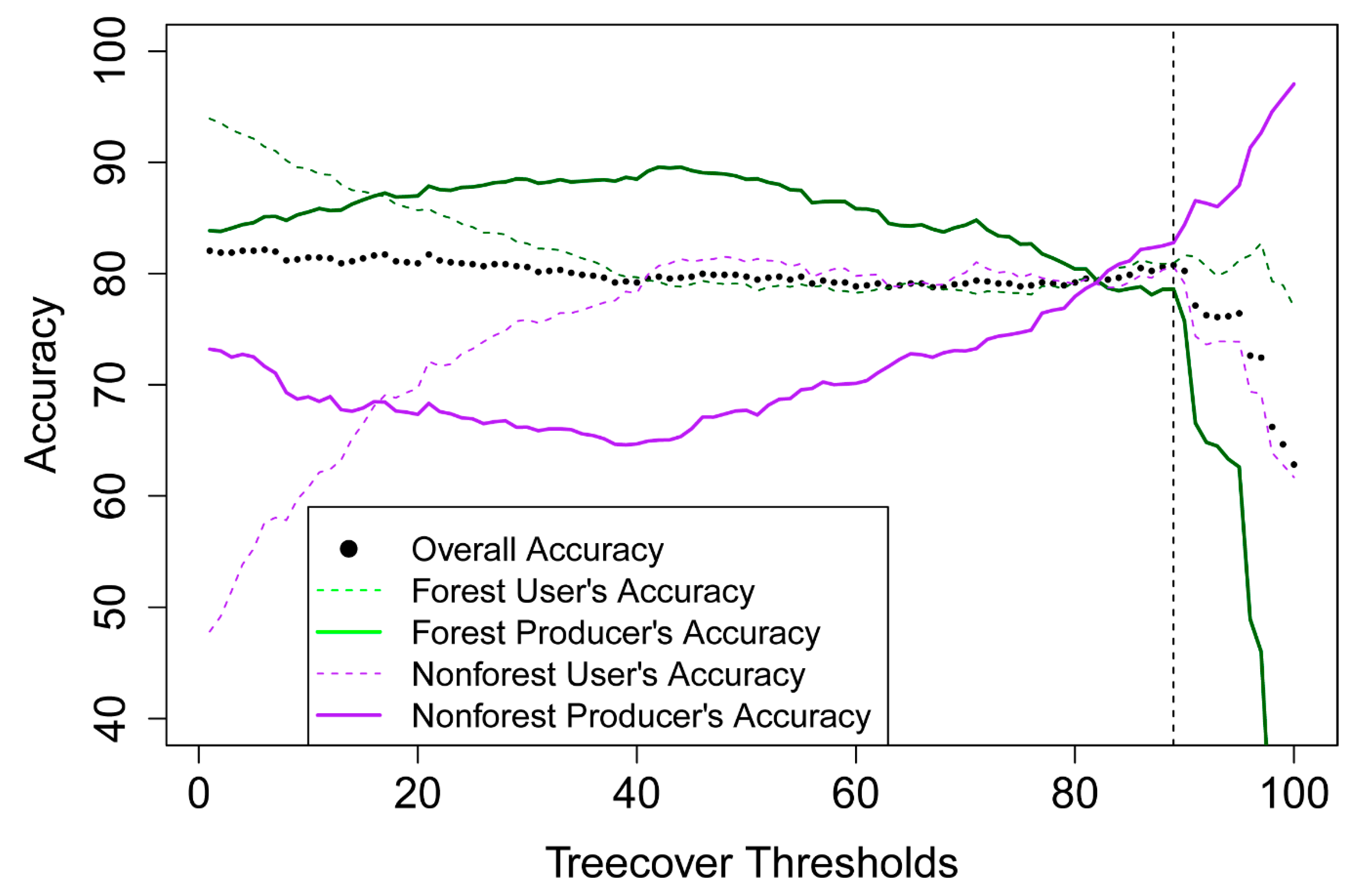
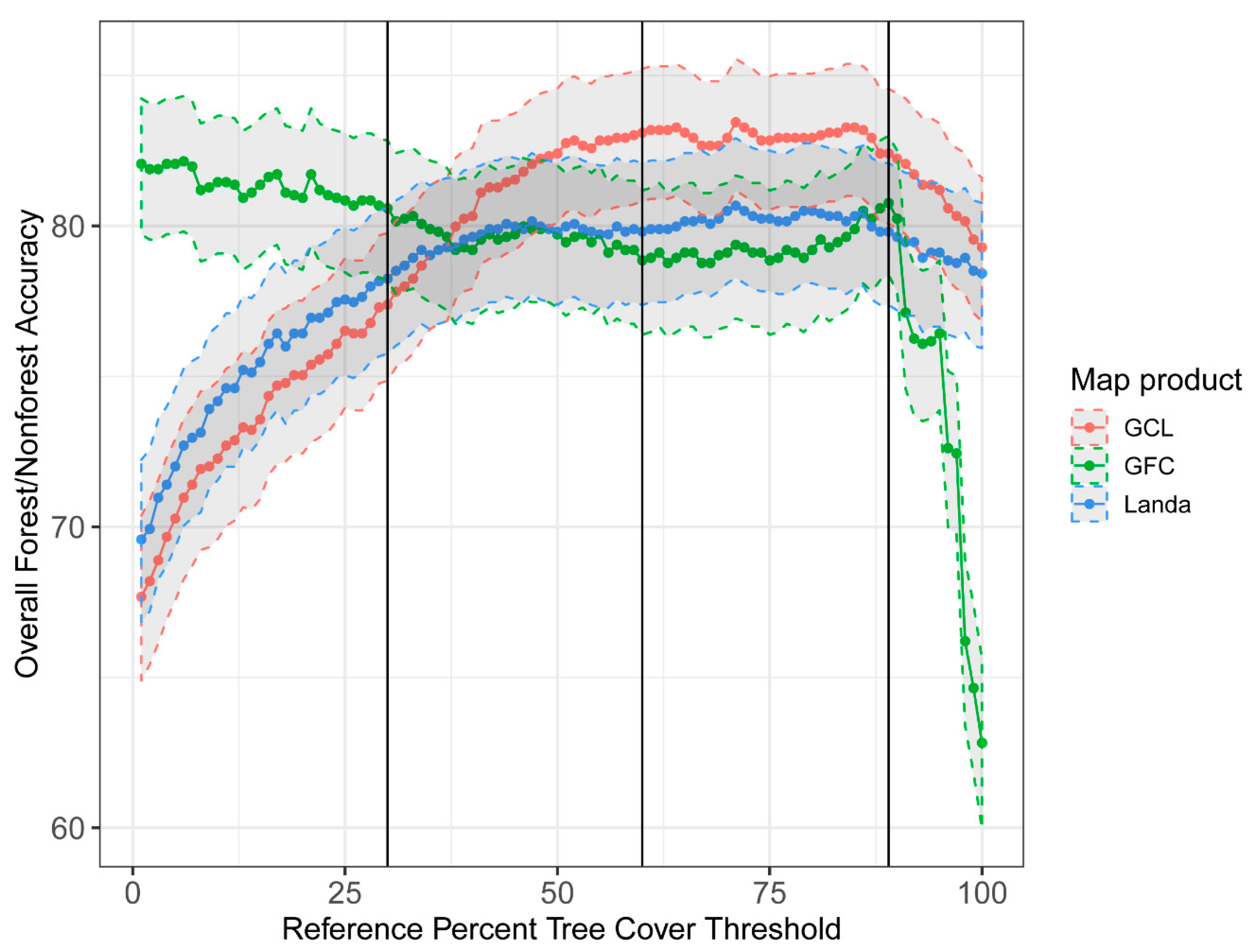
3.1. Tree Cover Threshold Analysis

The definition of forest cover, as expressed in the tree cover threshold for the reference data (1–100%), affected the absolute accuracy of the forest/non-forest maps by 20%–30% (Figure 1). However in general, the overall accuracy ranking of the maps relative to each other was consistent across tree cover thresholds ranging from 40% to 95% for (Figure 1). Across this range, the GCL map exceeded the GFC and Landa maps in overall accuracy, and the GFC and Landa maps had comparable accuracy. All three maps were comparable in accuracy at a 37% tree cover threshold. Below the 37% threshold, the Hansen map improved in overall accuracy while the forest/non-forest maps (GCL, Landa) degraded. Because of the overall consistency in relative rankings across a broad range of thresholds, we compared accuracy in detail across forest/non-forest maps only at the 89% tree cover threshold (see below and Table A1 for an accuracy comparison across three selected thresholds). Selecting a high reference threshold for forest cover in Costa Rica was also supported by reference assessments of tree cover in the visually classified forest land cover class, with a mean of 95% +/− 12% (mean +/− standard deviation (SD)).
Across all possible percent tree cover thresholds, we found that an 89% threshold on the GFC product resulted in the best balance of overall accuracy, class omission errors, and class commission errors in the resulting forest/non-forest map (Figure 2). This tree cover threshold was the highest overall accuracy in the region where both the GFC omission and omission errors differed by <5% between forest and non-forest classes. Thresholds greater than 89% reduced overall accuracy substantially, while thresholds less than 80% led to sharply declining commission and omission accuracies for the non-forest class. Although overall accuracy rose at lower thresholds, this resulted from non-forest reference pixels being less common at lower forest thresholds (by definition).

3.2. Global and Regional Map Accuracy

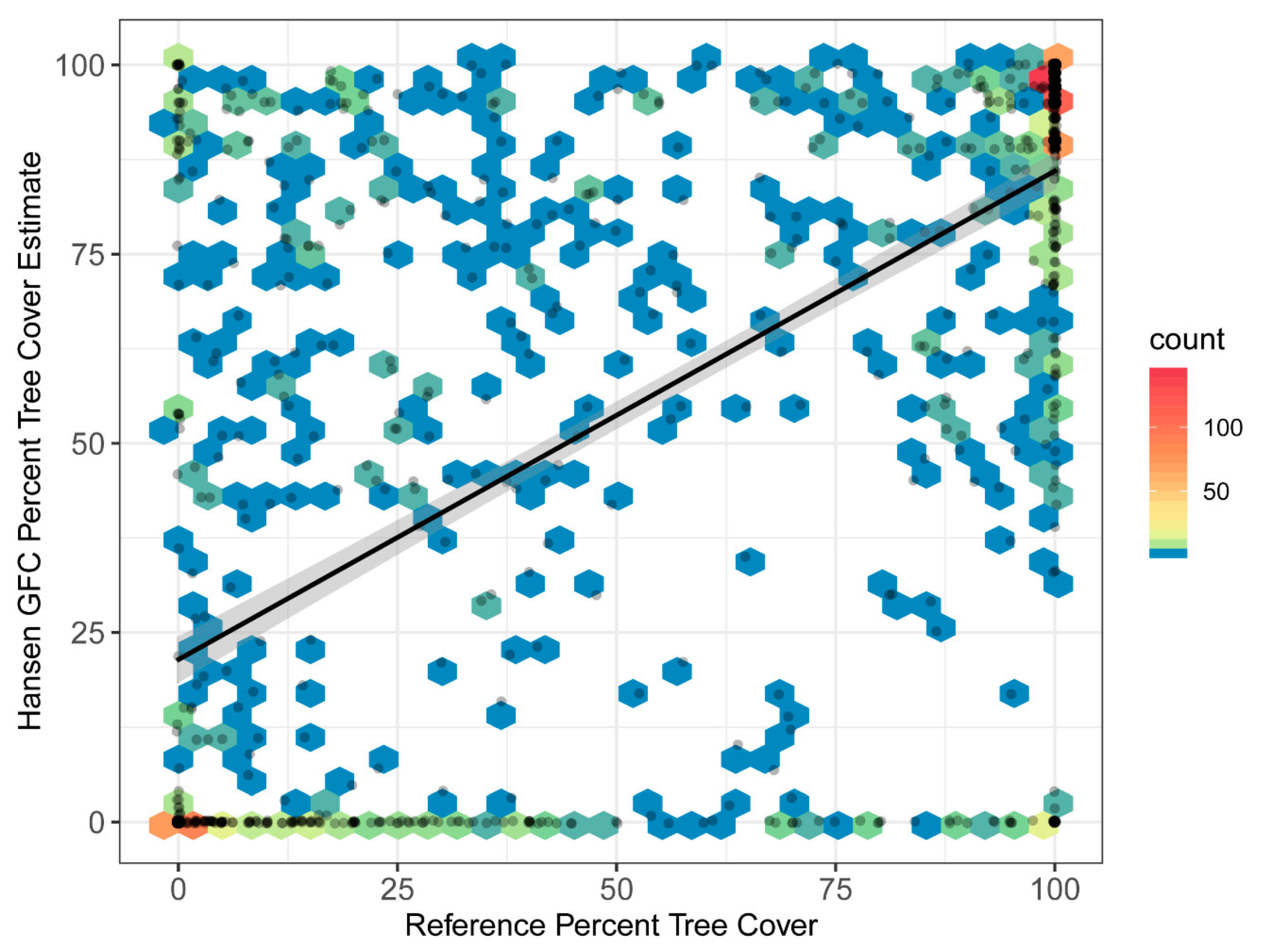
3.2.1. Accuracy of Continuous Tree Cover (GFC Only)

The global GFC percent tree cover product was able to predict a portion of the variation in the reference percent tree cover (Figure 3; linear regression, p < 0.0001, R2 = 0.44). Updating the GFC product from the year 2000 to the year 2015 slightly improved the overall accuracy (original 2000 data, linear regression, p < 0.0001, R2 = 0.42). The regressions were strongly influenced by the 0% and 100% reference values; omitting those values lowered predictive ability of both regressions (p < 0.0001, R2 = 0.11–0.13).

3.2.2. Comparing Forest/Non-forest Map Accuracy Across Tree Cover Products

When compared to the reference data (89% forest threshold), the Hansen global forest change product (89% forest threshold) had intermediate overall accuracy among the three products (80.8% +/− 2.3%; Table 3, Table A2). The spatial distribution of errors indicate that forest was underpredicted in the dry tropical forests of northwestern Costa Rica (Figure 4A,B). Forest was overpredicted in agricultural regions throughout Costa Rica, and particularly in banana and oil palm fields in the Atlantic and Pacific coastal plains. However, the GFC product appeared to predict small forest patches and narrow linear forest elements well across the entire country (Figure 4A, inset).
The derived GCL global forest map had the highest overall accuracy (82.2 +/− 2.2%; Table 3, Table A2). The map overpredicted forest cover (a user’s accuracy for forest of 77%). However, the spatial distribution of errors appeared to be uniform across the country, with no apparent spatial pattern to over-prediction or under-prediction of forest cover (Figure 5). Further inspection revealed that, despite its relatively small minimum mapping unit, the GCL product underpredicted and omitted small forest patches and linear forest elements (Figure 5 inset). However these small errors were not reflected in our reference data.
The Landa regional map had the lowest overall accuracy (79.3 +/− 2.4%; Table 3, Table A2) at the 89% threshold, although it was comparable to or slightly better than the GFC product across a wide range of tree cover thresholds (Figure 1). The map over-predicted forest cover (a user’s accuracy for forest of 75%), which might be expected of a map with a reported forest cover threshold of 30%. However, visual inspection showed localized areas of under-prediction where forests were classified as agriculture, typically around the edges of banana and coffee fields. The spatial distribution of overprediction errors appeared to be random (Figure 6), with a tendency to cluster along forest margins. Outside these clusters, a visual assessment indicated that the Landa map tended to under-predict forest cover in small patches and linear elements, as would be expected from a map with a one hectare minimum mapping unit.

3.3. Biases in Estimation of Tree Cover

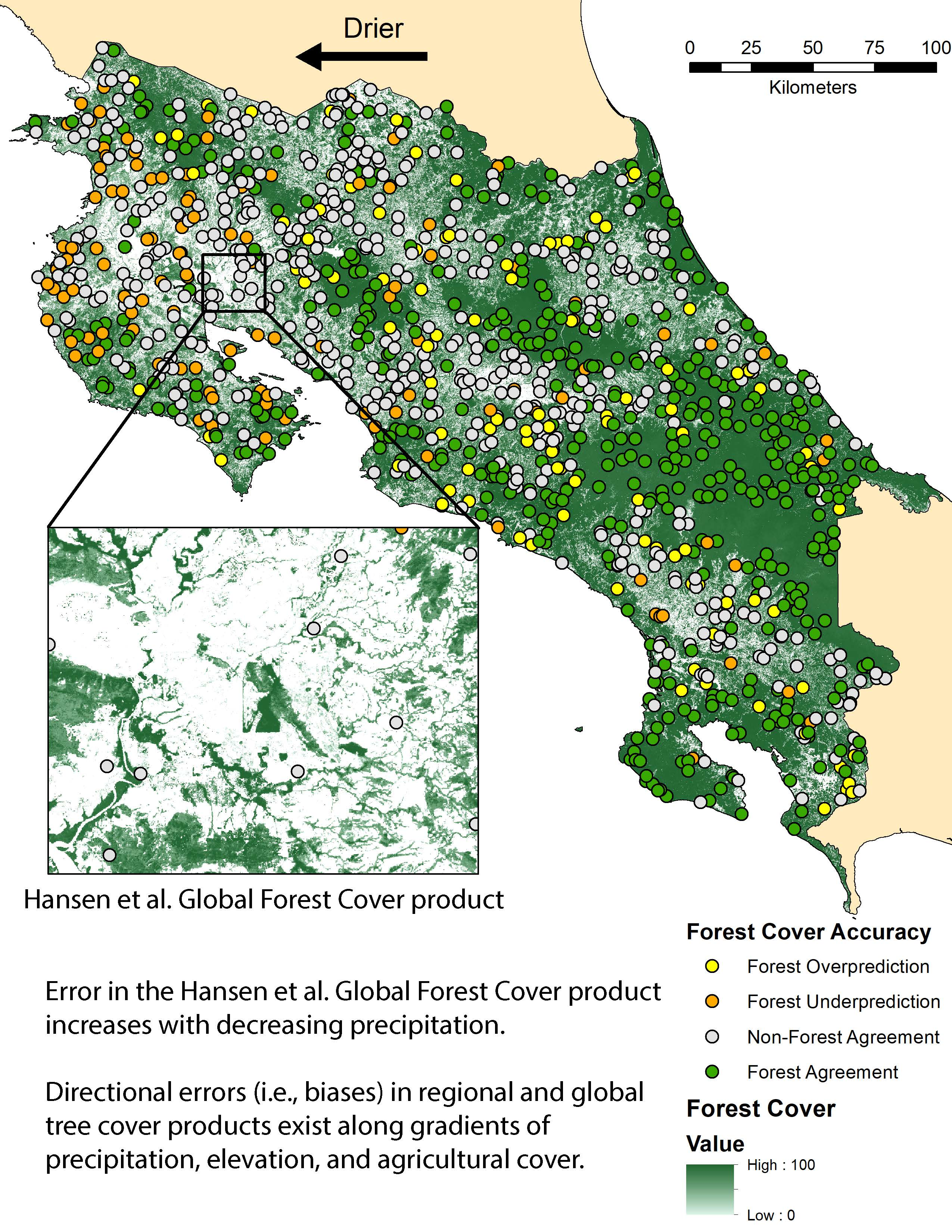
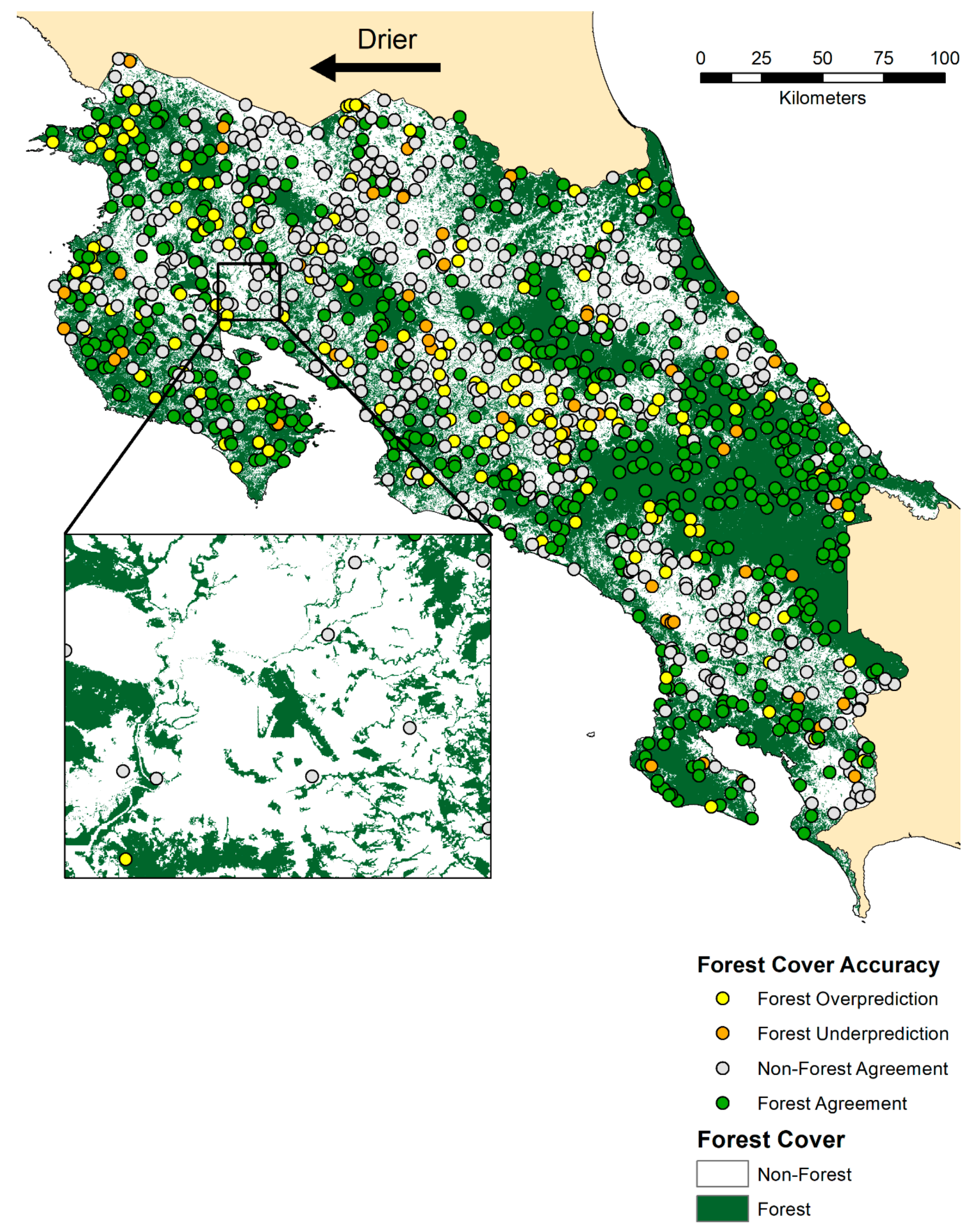
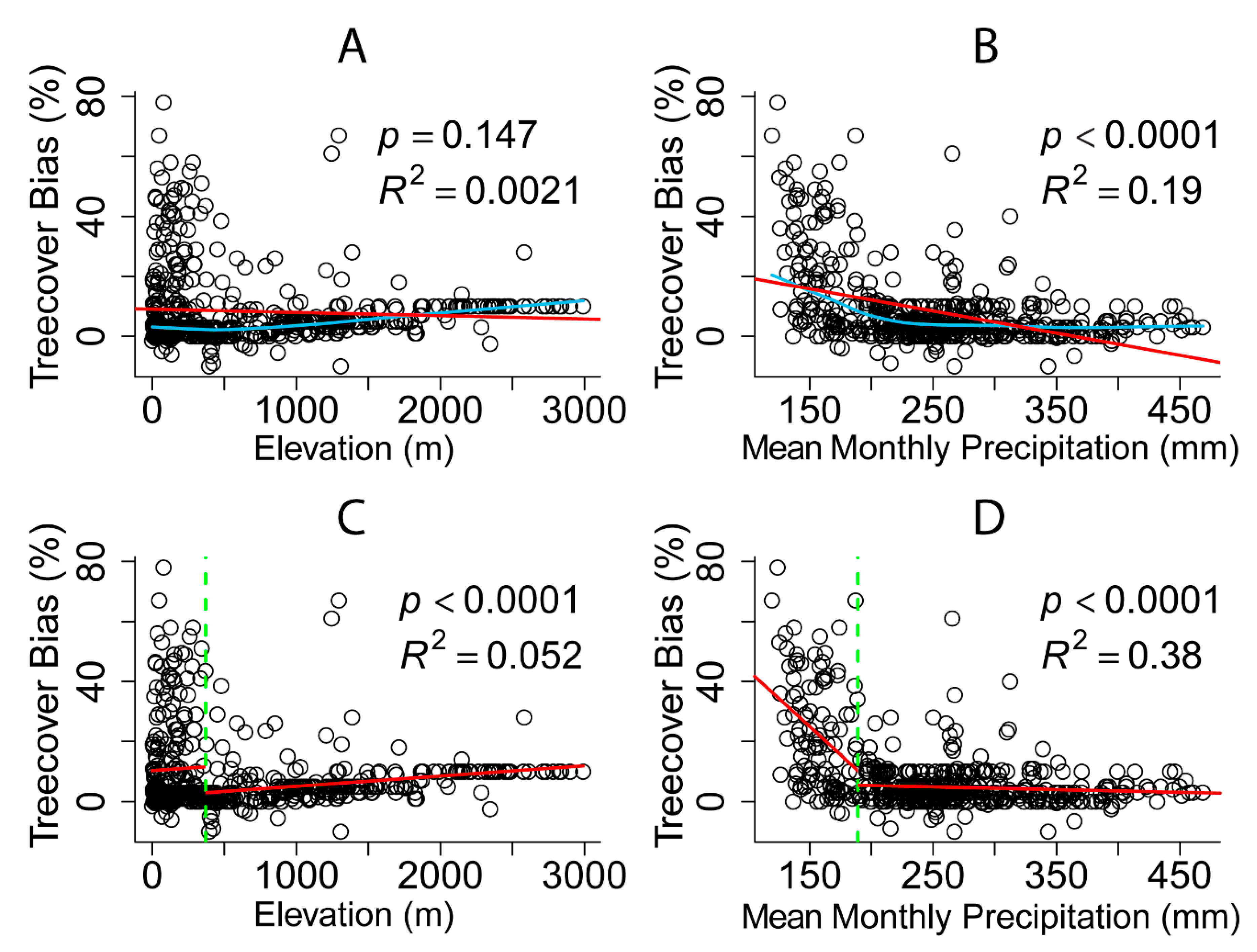
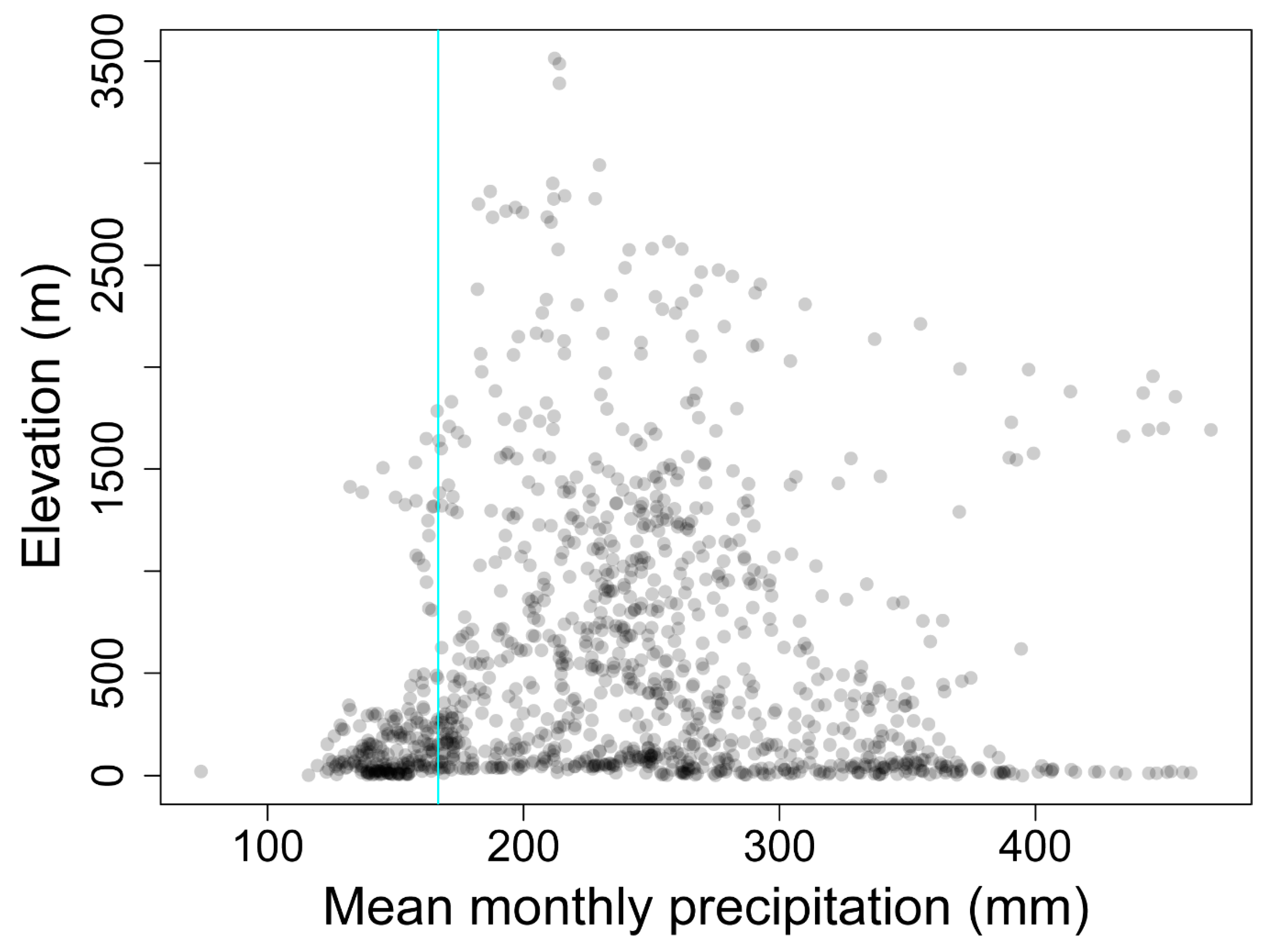
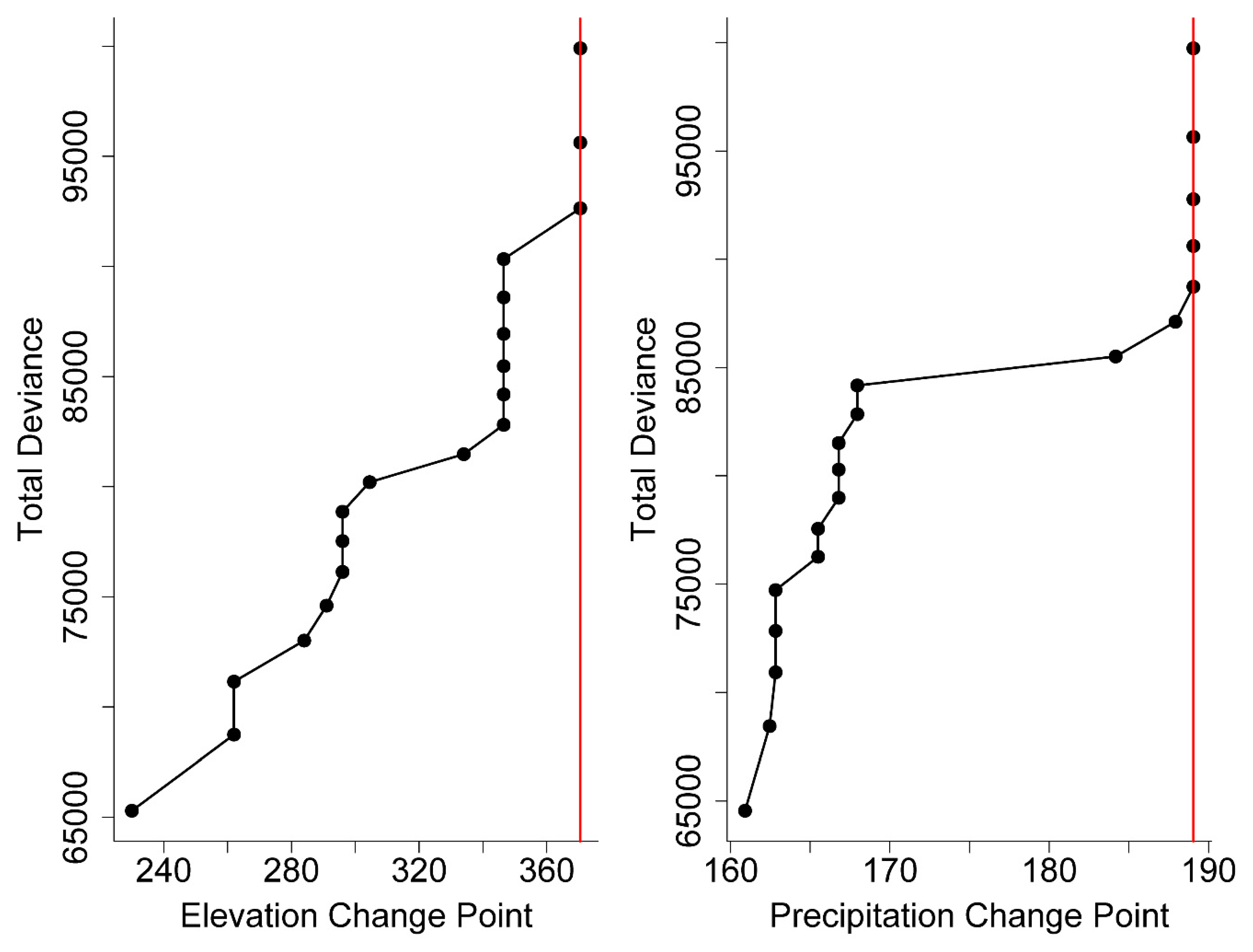
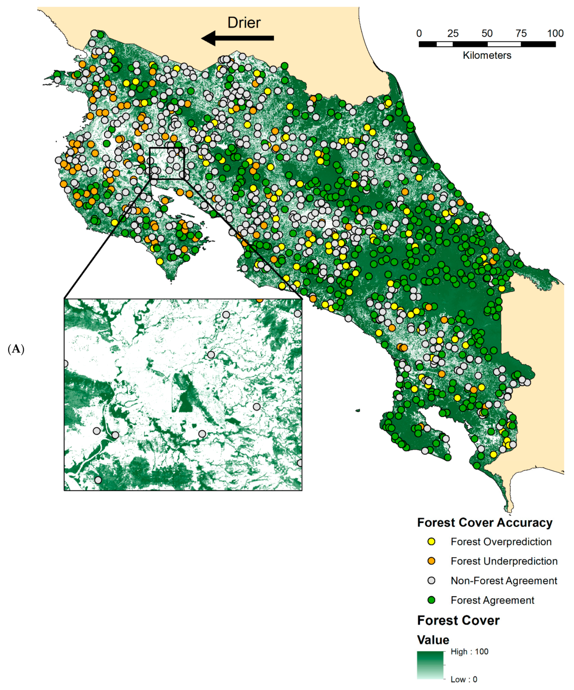
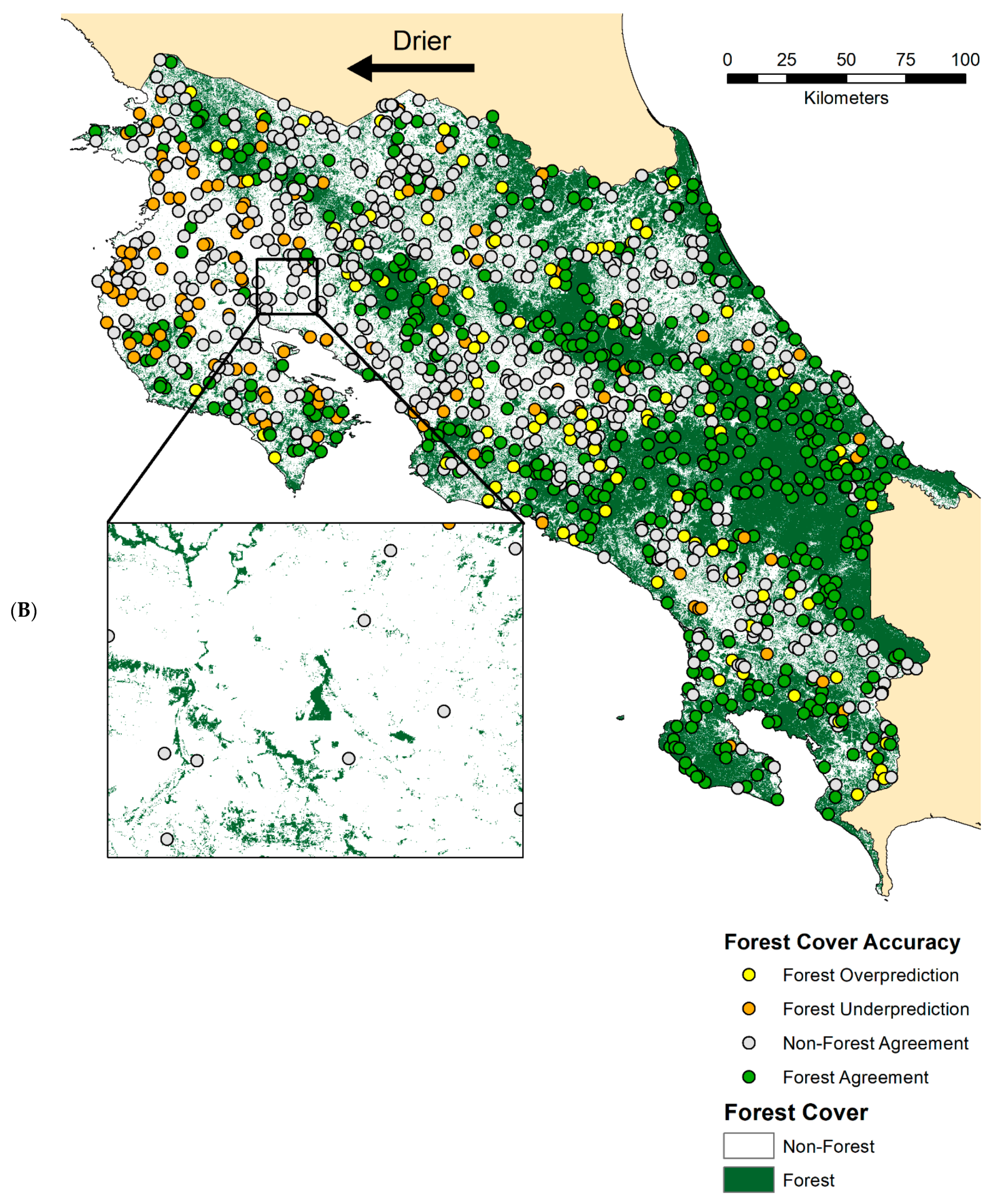
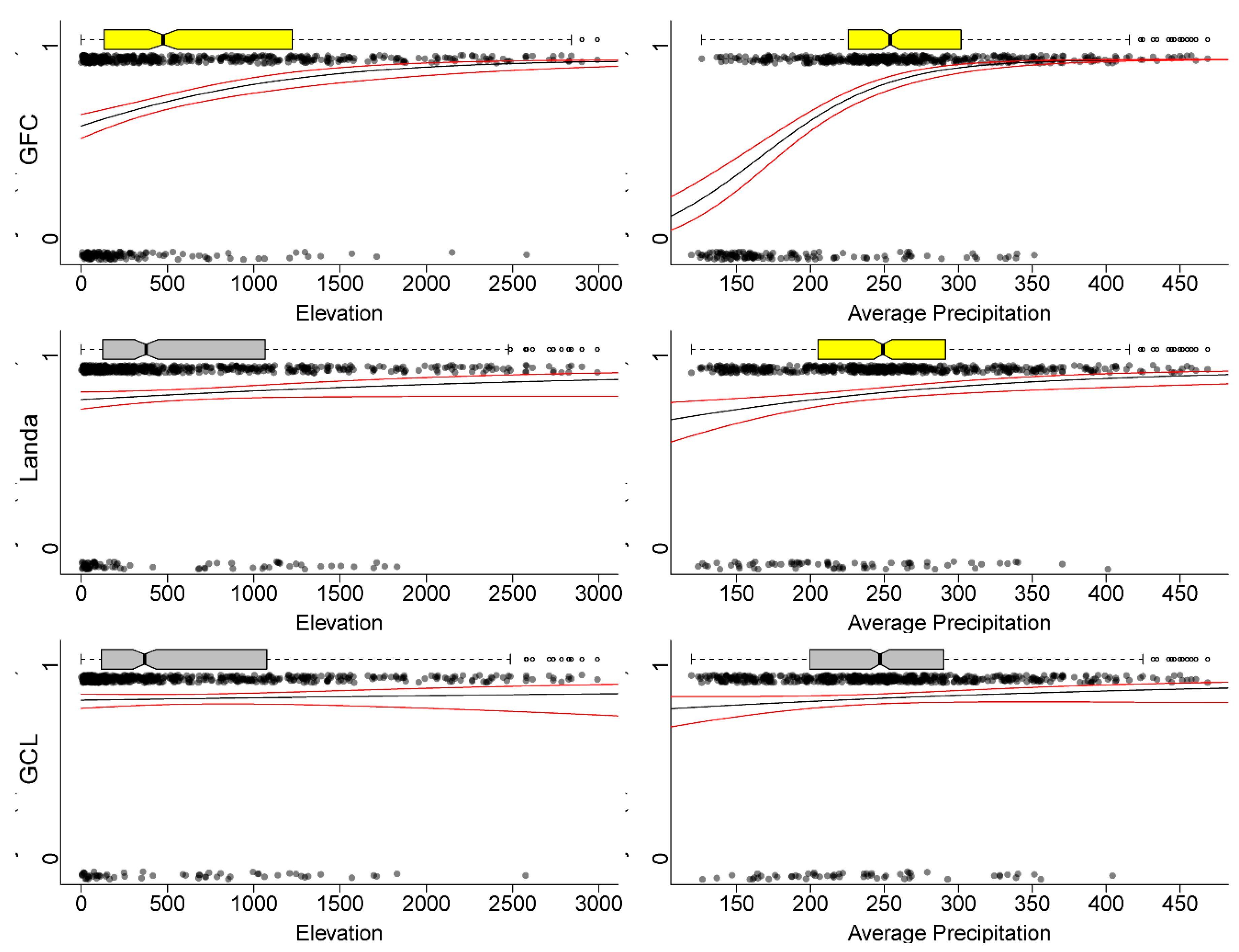
3.3.1. Forest/Non-forest Biases along Precipitation and Elevation Gradients

For non-forest reference data (<10% tree cover) analyzed by logistic regression, all products had small detectable biases in overestimating tree cover along elevation gradients. Tree cover was overestimated with increasing elevation, but the total effect was <1% over the range of elevation (p < 0.0002; Table A3). As precipitation decreased, only the GFC product was significantly less likely to predict tree cover in non-forest areas. This small precipitation effect in non-forest areas mirrored the stronger effect in forested areas (next paragraph), but weakened at increasing precipitation (p < 0.0007; Table A3).
For forest reference data (>89% tree cover) analyzed by logistic regression, neither the GCL or Landa forest products had detectable biases in underestimating tree cover along elevation gradients (Figure 7). For the GCL product, precipitation was not a significant predictor (p = 0.6, Table A4) of the probability of error in the forest/non-forest classification of forest reference points (i.e., the probability of a map predicting non-forest in forest reference pixels). The Landa product was significantly more likely to under-predict forest cover as precipitation declined, although the effect was small (Figure 7, Table A4).
In contrast, the GFC product had detectable bias in underestimating tree cover along both precipitation and elevation gradients (Figure 7). The likelihood of underprediction of forest cover increased at lower elevations (p < 0.0001) and drier conditions (p < 0.0001; Table A4). Low precipitation regions (i.e., tropical dry forest) were largely found at low elevations (0 m–370 m; Figure A1, Figure A2, Figure A3 and Figure A4), so it was not possible to meaningfully examine an interaction between elevation and precipitation.

3.3.2. GFC Tree Cover Biases along Precipitation and Elevation Gradients

For the GFC percentage tree cover estimates, there was tree cover bias with respect to elevation (Figure 8). Linear regressions fit to the testing data initially indicated no trend in error in tree cover estimates with respect to elevation (Figure 8A; p = 0.147; R2 = 0.0021, AIC = 4173). However, the relationship between elevation and bias was nonlinear, as indicated by the improved fit of the segmented linear regression (Figure 8C; p < 0.0001; R2 = 0.052, AIC = 4146). The nCPA identified 370.5 m as the 95th percentile changepoint (Figure A5). Below 370 m, mean levels of bias were significantly greater, likely because lowland dry forests were separated into this segment (Figure 8C; p < 0.0001). Above 370 m, tree cover in montane forests was underestimated by ~5% at 1000 m and by ~10% when elevation reached 2000 m (Figure 8C, Table A5). Although this additional bias above 370 m was not observed in our logistic regression results, this small elevation bias was found in >89% tree cover and largely occurred in intact montane forests with 100% actual cover. The logistic regression analysis used an 89% forest cover threshold, and therefore would not have been sensitive to a small underestimate of tree cover above 89% (e.g., a bias from 100% to 95%).
By contrast, the underestimation of tree cover by the GFC product was large at low precipitation levels. This precipitation bias is shown by a simple linear regression fit (Figure 8B; p < 0.0001, R2 = 0.19, AIC = 4065). However, the relationship between precipitation and bias was also nonlinear, as is shown by the improved fit of the segmented multiple linear regression (Figure 8D; p < 0.0001, R2 = 0.38, AIC = 3925). At precipitation levels below 189 mm, tree cover was underestimated by as much as 70%–80% when compared to the reference data (Figure 8D); 189 mm was identified as the 95th percentile changepoint in our nCPA analysis (Figure A5). Below this changepoint, the segmented regression slope was negative (p < 0.0001, precipitation effect, Table A3), while above 189 m, the regression slope did not differ from 0 (Figure 8D, Table A5).

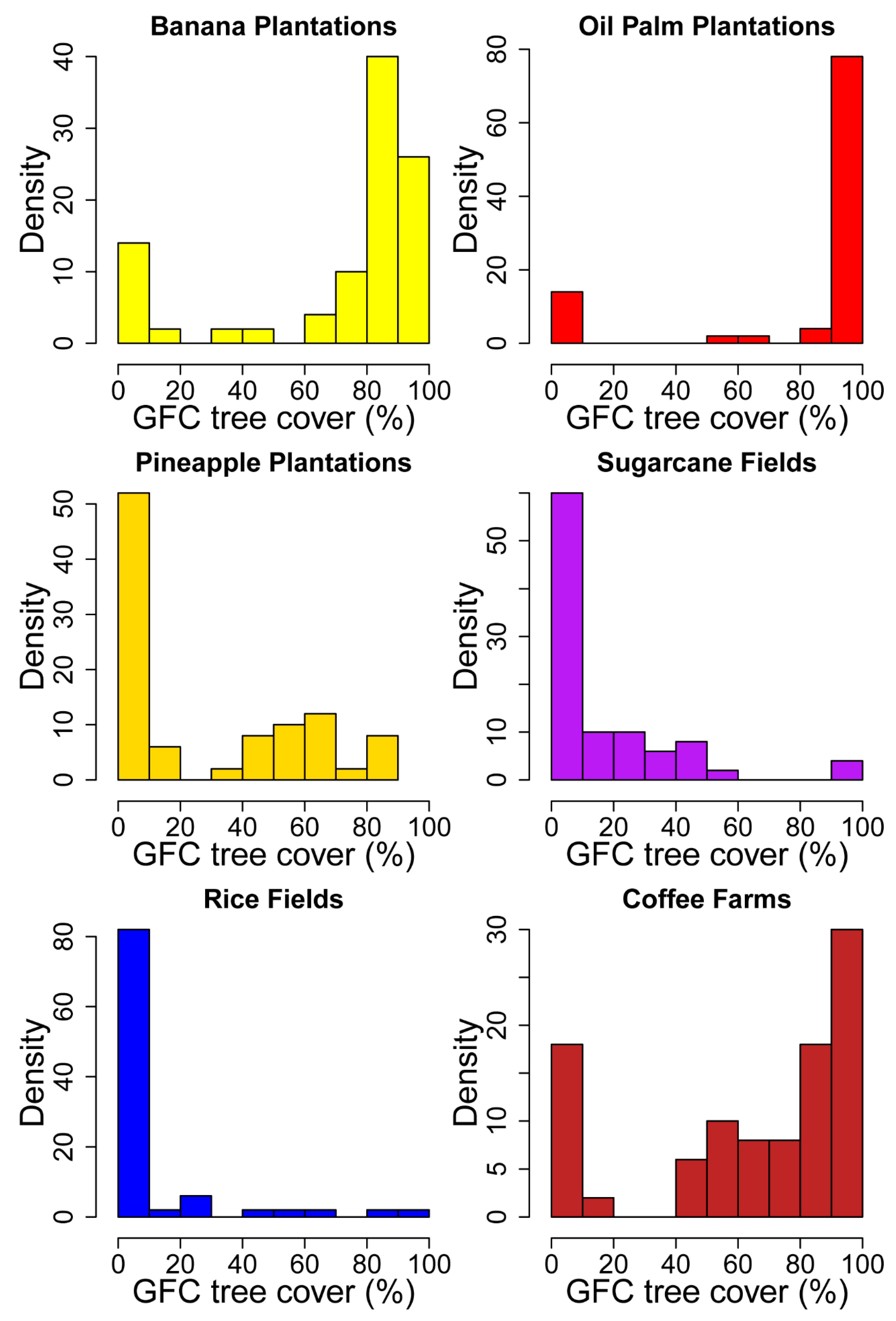
3.3.3. Tree Cover Biases along Agricultural Gradients

The GCL and Landa forest products only had small biases along agricultural gradients, with low rates of commission error over the most common crops in Costa Rica (Table 4). Less than 6% of agricultural validation points had tree cover for these two products, with the GCL slightly outperforming Landa on average (Table 4). Because the bias was relatively small, it did not affect our estimate for forest commission error in either map product. In our land cover validation data, both the GCL and Landa product never classified an agricultural area as forest. However, visual inspection of the Landa product indicated local underprediction of forest near agricultural fields that degraded its accuracy (for example, classifying forest as banana (non-forest)).
The GFC product, by contrast, had extensive tree cover bias in agriculture (Table 4, Figure 9). We found that 64% of the 300 agricultural points examined had tree cover greater than 0%, indicating widespread overprediction of forest cover across multiple crop types. At least 54% of the agriculture reference points had tree cover >30% in the GFC product (Table 4), and the maximum predicted tree cover values at a given pixel for each crop type ranged between 89% and 100% (Figure 9).

4. Discussion

4.1. Comparative Accuracy of Global and Local Tree Cover Products

Although our sample size of three forest products is small, this research directly challenges the assumption that regional maps are better than global maps. The regional Landa forest product examined in this study did not have better accuracy than either global tree cover product. We found that the global GCL product had considerably better accuracy than the regional product, despite a five-year difference between the reference data (2015) and the GCL product date (2010) that likely lowered its reported accuracy. The GFC accuracy was comparable to the regional map overall, and likely better than the regional map in the humid parts of Costa Rica. Relative to the regional Landa product, the GFC’s lower performance largely stemmed from underestimation of tree cover in dry tropical forests (Figure 4B) and in overestimation of tree cover in croplands.
Furthermore, a visual examination of the regional Landa product revealed large forest omission errors (i.e., forest incorrectly classified as agriculture) in the zones dominated by banana and coffee cultivation, respectively. The cause of the locally prevalent forest misclassification errors remains unclear, but could be related to insufficient training data or the Bayesian classifier used in their study [8]. Because these zones were not extensive across a large portion of Costa Rica, they did not have a major effect on overall accuracy. However, this misclassification and the resulting forest cover underestimation appears to persist across the entire Landa forest cover time series.
All forest products have their advantages and disadvantages, and should be used with caution [51]. Global forest products are consistent across boundaries, which allows forest cover to be compared between countries. However, even though the global GCL product outperformed the other products tested in terms of overall accuracy (Figure 1), its utility for global forest mapping is limited by several considerations. First, although the minimum mapping unit is small, it had restrictive connectivity requirements that meant thin forest elements were highly likely to be eliminated, even if they diagonally connected as part of a large forest patch [46]. As a result, omission errors in mapping small forest fragments and linear forest features were widespread. Second, the GCL product is not a time-series: This composite forest map was only created for 2010, so the forest cover estimates would need to be updated to monitor forest cover change. Finally, although the GCL is a global product, it differs among continents and the accuracy of this product was only tested regionally. Additional local accuracy assessments are needed to test this product outside Costa Rica.
Before a global or regional tree cover product is used, researchers need to determine if it best suits the needs of their analyses [51]. Despite the overall poor relative performance of the global GFC product, it was preferable to the GCL and Landa forest products in three respects. The first major advantage is that the GFC product measures percent tree cover. This gives the product versatility and flexibility, especially when countries define forest using percent canopy cover over a given area [39]. The legal definition of forest could be changed without requiring a new national forest map to be made, saving time and money. Second, commission errors for forest were higher for the GCL and Landa products; only the GFC predicted more non-forest than forest, as was found in our reference data. Third, our visual assessment indicated that the GFC product did the best job at predicting small forest elements and linear forest features, readily identifying isolated trees and tree cover outside forests (Figure 5, Figure 6 and Figure 7, insets). These forest features are quite important to analyses of fragmentation and connectivity [52,53].
It may be possible to create more accurate tree cover products by integrating regional and global approaches. For example, Sannier et al. [40] created a methodology to process the GFC product to match the land cover and the national definition of forest in Gabon, as the original GFC product over-predicted tree cover. In an innovative fusion approach, McRoberts et al. [41] input both global and regional tree cover maps as predictors in a statistical model to increase the accuracy of forest cover estimates in a region of Brazil. Both of these studies showed promising results in leveraging global products for more accurate regional forest maps, but the regions they mapped were relatively uniform in land cover and climate. In regions with significant biophysical gradients, further work may be necessary to integrate regional and global forest cover products.

4.2. Biases in Estimation of Tree Cover

The GCL global forest cover product and the regional Landa product did not strongly over-estimate or under-estimate tree cover along gradients of precipitation, elevation, or agricultural cover. However, the GFC product showed strong tree cover estimation bias across all three gradients. The GFC elevation bias was relatively small but consistently increased with elevation, rising to ~10% at >2000 m in elevation in Costa Rica. This bias could arise from noise artefacts introduced by terrain shadowing, persistent cloud cover at high elevation, cloud shadows [14,22,54,55], or semitransparent clouds [22,56]. Any of these artefacts could generate subpixel contamination in the composite imagery used to classify tree cover in the GFC product. In a comparison of global tree cover products across Africa, Gross et al. [57] found significant disagreement in tree cover predictions across mountainous terrain. Although this study focused on Costa Rica, tree cover underestimation at high elevations could potentially constitute a global artefact in the GFC product as shadowing and cloud cover in mountain ranges are ubiquitous [13].
Furthermore, the GFC product dramatically underestimated tree cover in dry tropical forests, especially when average monthly precipitation ranged from 74 mm to 189 mm. At this lowest range of precipitation, the GFC product underestimated tree cover by as much as 70%–80%. Although they did not quantify the degree of bias as precipitation declines, other global forest products have documented low accuracy in tropical dry forests [58], potentially for similar reasons. Taken together, the results of Sannier et al. [40] and Hojas-Gascon et al. [59] suggest that the GFC tends to overpredict tree cover in humid regions and under-predict tree cover in dry regions. Our results support this interpretation of their work. One possible explanation for the GFC’s underestimation of tree cover in dry tropical forests is that cloud-free, dry season Landsat imagery was likely preferred by the GFC’s Google Earth Engine Landsat compositing algorithm [5,58]. During the dry season, many dry tropical forest canopies senesce. Instead of estimating tree canopy cover, any dry season-dominated composite would estimate tree cover from understory conditions and evergreen tree cover.
If the results observed in our study hold globally, then estimates of tree cover from the GFC in tropical dry forests would be biased low. In drylands, Bastin et al. [15] showed that the Hansen GFC underestimated sparse forest area (<10% tree cover) by as much as a third. Staver and Hansen [60] argued that MODIS VCF products, which were used to create the GFC [5], should not be used below 30% tree cover. However the tropical dry forests examined here are less arid than the drylands in previous studies [61]; our work extends the known bias for the GFC product to ecosystems with much higher potential tree cover (100%) and carbon storage. If the trends observed here for estimating dry forest cover hold globally, then estimates that arise from tree cover (forest loss, forest gain, carbon storage, etc.; [62,63]) in dry forest ecosystems are likely also biased low.
In addition to the precipitation and elevation biases, the GFC product also committed errors in estimating tree cover within agricultural fields. Although banana, oil palm, and coffee crops were extensively classified as tree cover in the GFC product, this is partly to be expected from the GFC’s definition of “forest” (all vegetation taller than 5 m in height; [17,64]). However, it should also be noted that in this analysis the GFC product extensively predicted tree cover in short row crops like pineapple, rice, and sugarcane. Although Tropek et al. [17] anecdotally documented the existence of agricultural row crop errors, our sample is statistically robust and indicates much larger errors than previously observed. All row crops included error pixels with ≥89% tree cover (Figure 9), and sizeable fractions (between 10% and 86%) of each crop type had tree cover in excess of 30% (Table 4). The misclassified pixels do not represent edge pixels or mixed land covers, as the samples were taken from the interior of uniform fields.
Errors in row crop classification potentially resulted from using temporal dynamics in reflectance (i.e., greenness) as a predictor of tree cover [5], and may be most pronounced in tropical agricultural zones because of perennial agricultural cover. This may contribute to the small observed increase in tree cover estimates in open fields with increasing mean precipitation. Caution should be exercised when using the GFC product in fragmented agricultural landscapes dominated by row and tree crops [17]. In these landscapes, estimates of forest cover, fragmentation, connectivity and carbon storage may all be biased upwards. The importance and magnitude of agricultural cover errors in the GFC will likely worsen over time as croplands expand in the tropics [18,65]. These errors could be mitigated going forward by incorporating height and structural information from new lidar and radar data (e.g., [66,67]) into global forest products.
Although the GFC product has the advantage of being a time series of change in tree cover, its biases call into question the accuracy of its forest cover, gain, and loss products in agricultural landscapes and arid ecosystems. Planting and harvesting of crops could be interpreted as forest gain and loss, and this misclassification could deceive or be abused by local policy-makers and land managers making conservation decisions [17]. Furthermore, forest gain and loss may be underestimated in both drylands [63] and seasonally dry forests, calling into further question the utility of the GFC product for global forest monitoring outside humid regions. Our results indicate that the GFC product is most accurate in tropical regions with little relief, high, aseasonal rainfall, and low cropland area, such as the Amazon basin.

5. Conclusions

Researchers need to be careful when selecting forest cover products for analyses, as they vary in their ability to accurately map forest cover, fragmentation, and connectivity. Although the GFC product is the most widely used forest cover product for global and regional analyses, its accuracy was intermediate when compared to other forest products. The GCL product had the highest accuracy of all the products tested, challenging the assumption that regional map products are more accurate than global products. Biases in GFC tree cover estimates were found along gradients of precipitation, elevation, and agricultural cover. Global assessments need to be conducted to understand whether the observed GFC underpredictions of tree cover along biophysical gradients in Costa Rica have similar magnitudes elsewhere in the tropics. Since many forest product errors are spatially distributed, future research needs to account for spatial bias when attempting to analyze or generate forest products.

Supplementary Materials

The following are available online at https://www.mdpi.com/1999-4907/10/10/853/s1.

Author Contributions

These authors contributed to the following: conceptualization, methodology, formal analysis, investigation, writing—original draft preparation, writing—review and editing, and visualization, D.C.; M.E.F.; validation and data curation, D.C.; P.C.; supervision, project administration, and funding acquisition, M.E.F.

Funding

This research received no external funding.

Acknowledgments

We would like to thank Matthew Baker for technical and statistical guidance. We would also like to thank Maggie Holland for her feedback on earlier drafts of this manuscript.

Conflicts of Interest

The authors declare no conflict of interest.

Appendix A

In the main text, overall accuracy of the different map products is compared at different potential tree cover thresholds (1%–100%). For the GFC product only, we further compared detailed accuracies for each land cover class (i.e., forest or non-forest) at all possible thresholds. No one tree cover threshold is correct per se; all depends on the desired definition of forest cover. In the first part of this appendix section, we present the overall and class accuracies for each of the three different forest maps at three possible forest definitions: 30%, 60%, and 89% tree cover (Table A1). To do this, we compare predictions of the map product against reference locations where the tree cover is known. We then calculate accuracy using a confusion matrix that shows overall accuracy (%), the class user’s accuracy (100-commission error), and the class producer’s accuracy (100% omission error).
Table A1. Detailed confusion matrices showing the accuracy of different forest/non-forest maps at three forest cover thresholds (30%, 60%, and 89%). Producer’s accuracy and user’s accuracy are abbreviated below.
Reference data thresholded at 89%
GFC, 89% thresholdReference Data
PredictedNonforestForestTotalUser Acc.
Nonforest49511961480.6
Forest10343754080.9
Total5985561154Overall
Prod. Acc.82.878.6 80.8
GCLReference Data
PredictedNonforestForestTotalUser Acc.
Nonforest4515650789.0
Forest14750064777.3
Total5985561154Overall
Prod. Acc.75.489.9 82.4
LandaReference Data
PredictedNonforestForestTotalUser Acc.
Nonforest4367150786.0
Forest16248564775.0
Total5985561154Overall
Prod. Acc.72.987.2 79.8
Reference data thresholded at 60%
GFC, 60% thresholdReference Data
PredictedNonforestForestTotalUser Acc.
Nonforest3599145079.8
Forest15355170478.3
Total5126421154Overall
Prod. Acc.70.185.8 78.9
GCLReference Data
PredictedNonforestForestTotalUser Acc.
Nonforest4129550781.3
Forest10054764784.5
Total5126421154Overall
Prod. Acc.80.585.2 83.1
Reference data thresholded at 60%
LandaReference Data
PredictedNonforestForestTotalUser Acc.
Nonforest39311450777.5
Forest11952864781.6
Total5126421154Overall
Prod. Acc.76.882.2 79.8
Reference data thresholded at 30%
GFC, 30% thresholdReference Data
PredictedNonforestForestTotalUser Acc.
Nonforest2708635675.8
Forest13866079882.7
Total4087461154Overall
Prod. Acc.66.288.5 80.6
GCLReference Data
PredictedNonforestForestTotalUser Acc.
Nonforest32718050764.5
Forest8156664787.5
Total4087461154Overall
Prod. Acc.80.175.9 77.4
LandaReference Data
PredictedNonforestForestTotalUser Acc.
Nonforest33217550765.5
Forest7657164788.3
Total4087461154Overall
Prod. Acc.81.476.5 78.2
In the second part of this appendix section, we present area-corrected estimates of accuracy following the recommendations and methods of Olofsson et al. [68]. Taking the data presented in Table 3, along with the area of forest and non-forest in the land cover maps, we calculated revised estimates of accuracy and area (Table A2). Because both the area of forest and non-forest was relatively balanced across the maps, corrected overall accuracy had only minor differences with uncorrected accuracy (Table 3). For the Landa and GCL maps, the corrected area of non-forest was higher than the uncorrected estimate, and corrected omission errors for non-forest were correspondingly greater.
Table A2. Detailed, area-corrected confusion matrices showing the user’s, producer’s, and overall accuracy of different forest/non-forest maps at the 89% forest cover threshold. Overall accuracy and corrected area estimates are shown (mean +/− 95% confidence interval).
Reference data thresholded at 89%
GFC, 89% thresholdReference Data
PredictedNonforestForestTotalUser Acc.Original Map Area (km2)
Nonforest0.3940.09470.48980.629675
Forest0.0980.4140.51180.931049
Total0.4920.508 1OverallCorrected Area (km2)
Prod. Acc.80.281.4 80.8
+/− 2.3
NF: 29846 +/− 1387
For: 30878 +/− 1387
GCLReference Data
PredictedNonforestForestTotalUser Acc.Original Map Area (km2)
Nonforest0.3730.04630.41989.025451
Forest0.1320.4490.58177.235290
Total0.5050.4951 OverallCorrected Area (km2)
Prod. Acc.73.890.7 82.2
+/− 2.2
NF: 30658 +/− 1335
For: 30083 +/− 1335
LandaReference Data
PredictedNonforestForestTotalUser Acc.Original Map Area (km2)
Nonforest0.3370.05490.39286.023816
Forest0.1520.4560.60875.036908
Total0.4890.5111 OverallCorrected Area (km2)
Prod. Acc.68.989.2 79.8
+/− 2.4
NF: 29722 +/− 1428
For: 31002 +/− 1428

Appendix B

To examine bias in prediction of forest cover with respect to precipitation and elevation, we performed logistic regression analyses on all binary tree cover products, and linear regression analyses of the continuous product. Because low precipitation regions (<2000 mm annually, or 166.67 mm per month) primarily occurred at lower elevations, we could not meaningfully examine interactions between elevation and precipitation in any regression model predicting tree or forest cover (Figure A1, Figure A2, Figure A3 and Figure A4).
We first examined the probability of predicting forest cover in areas with <10% reference tree cover. We fit a full logistic regression model to the data, examining the effect of precipitation, elevation, and product type on forest cover presence (0 or 1). Precipitation and elevation, respectively, were allowed to interact with product type. The results show a significant general effect of elevation and a significant interaction between GFC and precipitation (Table A3). Forest was more likely to be predicted at higher elevation for all products, and for the GFC product, more likely to be predicted at higher precipitation.
Figure A1. Elevation across Costa Rica, with locations of reference data shown. Note the central mountain range running northwest–southeast.
Forests 10 00853 g0a1
Figure A2. Precipitation across Costa Rica, with locations of reference data shown. Note differences in rainfall between the east and west of the country.
Forests 10 00853 g0a2
Figure A3. Scatterplot of precipitation and elevation values at reference data locations across Costa Rica. Darker colors indicate higher densities of points, and the blue vertical line indicates precipitation of 2000 mm annually (~167 mm on average per month), the Holdridge threshold for the low-elevation dry forest biome.
Forests 10 00853 g0a3
Figure A4. GFC estimated tree cover across Costa Rica, displayed to emphasize bias patterns. Note differences in estimated tree cover between the east and west of the country; similar trends do not exist in the reference tree cover data, as noted in Figure 4A.
Forests 10 00853 g0a4
Table A3. Detailed model fit for the non-forest multiple logistic regression of the probability of predicted forest cover (0 or 1) against precipitation, elevation, and product type (GFC, Landa, and GCL). The data used for this analysis were non-forest reference data where tree cover was <10%.
Non-Forest Logistic Model (All Products)
PredictorsEstimateStd. Errorp-Value
Precipitation−0.00171440.0024150.4778
GFC product−4.00140350.6849305<0.0001
Landa product−2.9109780.6438071<0.0001
GCL product−1.57647060.5898350.0075
Elevation0.00082260.00022330.0002
Precipitation: GFC0.01029340.00341680.0026
Precipitation: Landa0.00532220.00341860.1195
Elevation: GFC−0.00050280.00034180.1413
Elevation: Landa−0.00023680.0003240.4647
We next examined the probability of predicting forest cover in areas with 89% or above reference tree cover. We fit a full logistic regression model to the data, examining the effect of precipitation, elevation, and product type on forest cover presence (0 or 1). Precipitation and elevation, respectively, were allowed to interact with product type. The full model results show a significant interaction between GFC and precipitation, and a significant interaction between GFC and elevation (Table A4). To further examine the performance of each tree cover product, we fit logistic regressions to each product to examine the probability of predicting forest as a function of elevation and precipitation. As seen in the full model, the GFC product was more likely to predict forest as elevation and precipitation increased, respectively. The Landa product was more likely to predict forest as precipitation increased, a result obscured in the full model (Table A4).
Table A4. Detailed model fits for the forest multiple logistic regressions of the probability of predicted forest cover (0 or 1) against precipitation, elevation, and product type. The data used for this analysis were forest reference data where tree cover was greater or equal to 89%. The full model fit is shown first, followed by individual model fits for each of the three tree cover products (GFC, Landa, and GCL).
Forest Logistic Model (All Products)
PredictorsEstimateStd. Errorp-Value
Precipitation0.0033030.0020480.1068
GCL product1.3240.50450.0087
GFC product−3.6510.4903<0.0001
Landa product0.29890.45480.511
Elevation0.000098150.00020870.6382
Precipitation: GFC0.016360.003107<0.0001
Precipitation: Landa0.0027220.0028210.3347
Elevation: GFC0.00087940.00032620.007
Elevation: Landa0.00021650.00029540.4636
Forest Logistic Model (GFC Product)
PredictorsEstimateStd. Errorp-Value
(Intercept)0.11120.055370.0451
Precipitation0.0023660.0002089<0.0001
Elevation0.00012570.00002141<0.0001
Forest Logistic Model (Landa Product)
PredictorsEstimateStd. Errorp-Value
(Intercept)0.69270.05092<0.0001
Precipitation0.00062980.00019210.0011
Elevation0.000033450.000019690.0899
Forest Logistic Model (GCL Product)
PredictorsEstimateStd. Errorp-Value
(Intercept)0.82140.04638<0.0001
Precipitation0.00028680.0001750.102
Elevation0.0000093980.000017930.6
To further examine bias in the GFC product, we fit two segmented linear regressions to the calculated bias (Reference tree cover (%) − GFC tree cover (%)) with elevation and precipitation, respectively, as predictors. Nonparametric changepoint analysis (nCPA detected potential nonlinear change thresholds in bias along the precipitation and elevation gradients, respectively. To account for uncertainty in the change point estimation, the 95% quantiles of potential change thresholds were selected as changepoints (Figure A5; 370.5 m for elevation, 189.04 mm for precipitation). The dataset was then labeled by segmented relative to the changepoint (above/below), and thus the segment was included as a factor predictor in each model.
Figure A5. Plots of nonparametric changepoint analysis (nCPA) quantiles, showing the total deviance at each possible changepoint split. Each point is a quantile (every 5%) of the distribution of changepoints from the nCPA analysis bootstrap, with the exact changepoint value on the x-axis. The red line indicates the changepoint values selected for the segmented regressions on elevation and precipitation, respectively.
Forests 10 00853 g0a5
For elevation, three models were compared: (1) Elevation alone, (2) elevation and segment (i.e., slope constant on both sides of segment, intercept varies), and (3) elevation interacts with segment (intercept and slope vary on each side of segment). The best-fit model (ΔAIC = −1.484) was the second (slope constant, intercept varies; Table A5).
Table A5. Detailed model fits for the segmented multiple linear regressions of GFC tree cover against precipitation and segment, and elevation and segment, respectively. The best-fit model for elevation did not include an interaction with segment, while the best-fit model for precipitation included an interaction with segment.
Segmented Linear Regression Model, Elevation
PredictorsEstimateStd. Errorp-Value
(Intercept)10.3218450.765543<0.0001
Elevation0.0034150.0011110.0022
Segment−8.6307461.607162<0.0001
Segmented Linear Regression Model, Precipitation
PredictorsEstimateStd. Errorp-Value
(Intercept)81.224938.71178<0.0001
Segment−74.113218.99691<0.0001
Precipitation−0.375080.055<0.0001
Precipitation:Segment0.366210.05557<0.0001
For precipitation, three models were compared: (1) Precipitation alone, (2) precipitation and segment (i.e., slope constant on both sides of segment, intercept varies), and (3) precipitation interacting with segment (intercept and slope vary on each side of segment). The best-fit model (ΔAIC = −40.05) was the third (slope and intercept vary; Table A5). The segment effect is essentially an adjustment to the regression intercept to the right of the segment point.

References

  1. Wright, S.J. Tropical forests in a changing environment. Trends Ecol. Evol. 2005, 20, 553–560. [Google Scholar] [CrossRef] [PubMed]
  2. Defries, R.; Hansen, A.; Newton, A.C.; Hansen, M.C. Increasing Isolation of Protected Areas in Tropical Forests Over the Past Twenty Years. Ecol. Appl. 2005, 15, 19–26. [Google Scholar] [CrossRef]
  3. Gardner, T.A.; Barlow, J.; Chazdon, R.; Ewers, R.M.; Harvey, C.A.; Peres, C.A.; Sodhi, N.S. Prospects for tropical forest biodiversity in a human-modified world. Ecol. Lett. 2009, 12, 561–582. [Google Scholar] [CrossRef] [PubMed] [Green Version]
  4. Laurance, W.F.; Useche, D.C.; Rendeiro, J.; Kalka, M.; Bradshaw, C.J.A.; Sloan, S.P.; Laurance, S.G.; Campbell, M.; Abernethy, K.; Alvarez, P.; et al. Averting biodiversity collapse in tropical forest protected areas. Nature 2012, 489, 290. [Google Scholar] [CrossRef]
  5. Hansen, M.C.; Potapov, P.V.; Moore, R.; Hancher, M.; Turubanova, S.A.; Tyukavina, A.; Thau, D.; Stehman, S.V.; Goetz, S.J.; Loveland, T.R.; et al. High-resolution global maps of 21st-century forest cover change. Science 2013, 342, 850–853. [Google Scholar] [CrossRef]
  6. Saatchi, S.S.; Harris, N.L.; Brown, S.; Lefsky, M.; Mitchard, E.T.A.; Salas, W.; Zutta, B.R.; Buermann, W.; Lewis, S.L.; Hagen, S.; et al. Benchmark map of forest carbon stocks in tropical regions across three continents. Proc. Natl. Acad. Sci. USA 2011, 108, 9899–9904. [Google Scholar] [CrossRef] [Green Version]
  7. Gibbs, H.K.; Brown, S.; Niles, J.O.; Foley, J.A. Monitoring and estimating tropical forest carbon stocks: Making REDD a reality. Environ. Res. Lett. 2007, 2, 045023. [Google Scholar] [CrossRef]
  8. Fernández-Landa, A.; Algeet-Abarquero, N.; Fernández-Moya, J.; Guillén-Climent, M.; Pedroni, L.; García, F.; Espejo, A.; Villegas, J.; Marchamalo, M.; Bonatti, J.; et al. An Operational Framework for Land Cover Classification in the Context of REDD+ Mechanisms. A Case Study from Costa Rica. Remote Sens. 2016, 8, 593. [Google Scholar] [CrossRef]
  9. DeFries, R.; Hansen, M.; Townshend, J. Global discrimination of land cover types from metrics derived from AVHRR pathfinder data. Remote Sens. Environ. 1995, 54, 209–222. [Google Scholar] [CrossRef]
  10. Sexton, J.O.; Song, X.-P.; Feng, M.; Noojipady, P.; Anand, A.; Huang, C.; Kim, D.-H.; Collins, K.M.; Channan, S.; DiMiceli, C. Global, 30-m resolution continuous fields of tree cover: Landsat-based rescaling of MODIS Vegetation Continuous Fields with lidar-based estimates of error. Int. J. Digit. Earth 2013, 6, 427–448. [Google Scholar] [CrossRef]
  11. Fagan, M.E.; DeFries, R.S. Measurement and Monitoring of the World’s Forests: A Review and Summary of Technical Capability, 2009–2015; Resources for the Future (RFF): Washington, DC, USA, 2009. [Google Scholar]
  12. Young, N.E.; Anderson, R.S.; Chignell, S.M.; Vorster, A.G.; Lawrence, R.; Evangelista, P.H. A survival guide to Landsat preprocessing. Ecology 2017, 98, 920–932. [Google Scholar] [CrossRef] [PubMed] [Green Version]
  13. Wilson, A.M.; Jetz, W. Remotely Sensed High-Resolution Global Cloud Dynamics for Predicting Ecosystem and Biodiversity Distributions. PLoS Biol. 2016, 14, e1002415. [Google Scholar] [CrossRef] [PubMed]
  14. Asner, G.P. Cloud cover in Landsat observations of the Brazilian Amazon. Int. J. Remote Sens. 2001, 22, 3855–3862. [Google Scholar] [CrossRef]
  15. Bastin, J.-F.; Berrahmouni, N.; Grainger, A.; Maniatis, D.; Mollicone, D.; Moore, R.; Patriarca, C.; Picard, N.; Sparrow, B.; Abraham, E.M.M.; et al. The extent of forest in dryland biomes. Science 2017, 356, 635–638. [Google Scholar] [CrossRef] [PubMed] [Green Version]
  16. Kalacska, M.; Sanchez-Azofeifa, G.A.; Rivard, B.; Caelli, T.; White, H.P.; Calvo-Alvarado, J.C. Ecological fingerprinting of ecosystem succession: Estimating secondary tropical dry forest structure and diversity using imaging spectroscopy. Remote Sens. Environ. 2007, 108, 82–96. [Google Scholar] [CrossRef]
  17. Tropek, R.; Beck, J.; Keil, P.; Musilová, Z.; Irena, Š.; Storch, D.; Sedláček, O.; Beck, J.; Keil, P.; Musilová, Z.; et al. Comment on “High-resolution global maps of 21st-century forest cover change”. Science 2014, 344, 981. [Google Scholar] [CrossRef] [PubMed]
  18. Laurance, W.F.; Sayer, J.; Cassman, K.G. Agricultural expansion and its impacts on tropical nature. Trends Ecol. Evol. 2014, 29, 107–116. [Google Scholar] [CrossRef] [PubMed]
  19. Fitzherbert, E.B.; Struebig, M.J.; Morel, A.; Danielsen, F.; Brühl, C.A.; Donald, P.F.; Phalan, B. How will oil palm expansion affect biodiversity? Trends Ecol. Evol. 2008, 23, 538–545. [Google Scholar] [CrossRef]
  20. Hansen, M.C.; Roy, D.P.; Lindquist, E.; Adusei, B.; Justice, C.O.; Altstatt, A. A method for integrating MODIS and Landsat data for systematic monitoring of forest cover and change in the Congo Basin. Remote Sens. Environ. 2008, 112, 2495–2513. [Google Scholar] [CrossRef]
  21. Harper, G.J.; Steininger, M.K.; Tucker, C.J.; Juhn, D.; Hawkins, F. Fifty years of deforestation and forest fragmentation in Madagascar. Environ. Conserv. 2007, 34, 325–333. [Google Scholar] [CrossRef]
  22. Zhu, Z.; Woodcock, C.E. Object-based cloud and cloud shadow detection in Landsat imagery. Remote Sens. Environ. 2012, 118, 83–94. [Google Scholar] [CrossRef]
  23. Hilker, T.; Lyapustin, A.I.; Tucker, C.J.; Hall, F.G.; Myneni, R.B.; Wang, Y.; Bi, J.; Mendes de Moura, Y.; Sellers, P.J. Vegetation dynamics and rainfall sensitivity of the Amazon. Proc. Natl. Acad. Sci. USA 2014, 111, 16041–16046. [Google Scholar] [CrossRef] [PubMed] [Green Version]
  24. Morton, D.C.; Nagol, J.; Carabajal, C.C.; Rosette, J.; Palace, M.; Cook, B.D.; Vermote, E.F.; Harding, D.J.; North, P.R.J. Amazon forests maintain consistent canopy structure and greenness during the dry season. Nature 2014, 506, 221–224. [Google Scholar] [CrossRef] [PubMed]
  25. Huete, A.R.; Didan, K.; Shimabukuro, Y.E.; Ratana, P.; Saleska, S.R.; Hutyra, L.R.; Yang, W.; Nemani, R.R.; Myneni, R.B. Amazon rainforests green-up with sunlight in dry season. Geophys. Res. Lett. 2006, 33, 2–5. [Google Scholar] [CrossRef]
  26. La Barreda-Bautista, B.D.; López-Caloca, A.A.; Couturier, S.; Silván-Cárdenas, J.L. Tropical Dry Forests in the Global Picture: The Challenge of Remote Sensing-Based Change Detection in Tropical Dry Environments; Intechopen: London, UK, 2011. [Google Scholar]
  27. Arroyo-Mora, J.P.; Sánchez-Azofeifa, G.A.; Kalacska, M.; Rivard, B.; Calvo-Alvarado, J.C.; Janzen, D.H. Secondary forest detection in a neotropical dry forest landscape using landsat 7 ETM + and IKONOS Imagery. Biotropica 2005, 37, 497–507. [Google Scholar] [CrossRef]
  28. Da Rocha, H.R.; Goulden, M.L.; Miller, S.D.; Menton, M.C.; Pinto, L.D.V.O.; De Freitas, H.C.; E. Silva Figueira, A.M. Seasonality of water and heat fluxes over a tropical forest in eastern Amazonia. Ecol. Appl. 2004, 14, 22–32. [Google Scholar] [CrossRef]
  29. Feng, X.; Porporato, A.; Rodriguez-Iturbe, I. Changes in rainfall seasonality in the tropics. Nat. Clim. Chang. 2013, 3, 811–815. [Google Scholar] [CrossRef]
  30. Lopes, A.P.; Nelson, B.W.; Wu, J.; de Alencastro Graça, P.M.L.; Tavares, J.V.; Prohaska, N.; Martins, G.A.; Saleska, S.R. Leaf flush drives dry season green-up of the Central Amazon. Remote Sens. Environ. 2016, 182, 90–98. [Google Scholar] [CrossRef]
  31. Smith, N.J.; Williams, J.T.; Plucknett, D.L.; Talbot, J.P. Tropical Forests and Their Crops; Cornell University Press: Ithaca, NY, USA, 2018. [Google Scholar]
  32. Grainger, A. Difficulties in tracking the long-term global trend in tropical forest area. Proc. Natl. Acad. Sci. USA 2008, 105, 818–823. [Google Scholar] [CrossRef] [PubMed] [Green Version]
  33. Chazdon, R.L. Beyond deforestation: Restoring forests and ecosystem services on degraded lands. Science 2008, 320, 1458–1460. [Google Scholar] [CrossRef]
  34. Bremer, L.L.; Farley, K.A. Does plantation forestry restore biodiversity or create green deserts? A synthesis of the effects of land-use transitions on plant species richness. Biodivers. Conserv. 2010, 19, 3893–3915. [Google Scholar] [CrossRef] [Green Version]
  35. Puyravaud, J.P.; Davidar, P.; Laurance, W.F. Cryptic destruction of India’s native forests. Conserv. Lett. 2010, 3, 390–394. [Google Scholar] [CrossRef]
  36. Phillips, H.R.P.; Newbold, T.; Purvis, A. Land-use effects on local biodiversity in tropical forests vary between continents. Biodivers. Conserv. 2017, 26, 2251–2270. [Google Scholar] [CrossRef] [Green Version]
  37. Barrett, F.; Mcroberts, R.E.; Tomppo, E.; Cienciala, E.; Waser, L.T. Remote Sensing of Environment A questionnaire-based review of the operational use of remotely sensed data by national forest inventories. Remote Sens. Environ. 2016, 174, 279–289. [Google Scholar] [CrossRef]
  38. Herold, M. An Assessment of National Forest Monitoring Capabilities in Tropical Non-Annex I Countries: Recommendations for Capacity Building; Center for International Forestry Research: Bogor, Indonesia, 2009. [Google Scholar]
  39. Sexton, J.O.; Noojipady, P.; Song, X.-P.; Feng, M.; Song, D.-X.; Kim, D.-H.; Anand, A.; Huang, C.; Channan, S.; Pimm, S.L.L.; et al. Conservation policy and the measurement of forests. Nat. Clim. Chang. 2015, 6, 192–196. [Google Scholar] [CrossRef]
  40. Sannier, C.; McRoberts, R.E.; Fichet, L.-V. Suitability of Global Forest Change data to report forest cover estimates at national level in Gabon. Remote Sens. Environ. 2016, 173, 326–338. [Google Scholar] [CrossRef]
  41. McRoberts, R.E.; Vibrans, A.C.; Sannier, C.; Næsset, E.; Hansen, M.C.; Walters, B.F.; Lingner, D. V Methods for evaluating the utilities of local and global maps for increasing the precision of estimates of subtropical forest area. Can. J. For. Res. 2016, 924, 924–932. [Google Scholar] [CrossRef]
  42. Pfaff, A.; Robalino, J.A.; Sanchez-Azofeifa, G.A. Payments for Environmental Services: Empirical Analysis for Costa Rica; Terry Sanford Institute of Public Policy, Duke University: Durham, NC, USA, 2007; pp. 404–424. [Google Scholar]
  43. Arroyo-Mora, J.P.; Sánchez-Azofeifa, G.A.; Rivard, B.; Calvo, J.C.; Janzen, D.H. Dynamics in landscape structure and composition for the Chorotega region, Costa Rica from 1960 to 2000. Agric. Ecosyst. Environ. 2005, 106, 27–39. [Google Scholar] [CrossRef]
  44. Holdridge, L.R.; Grenke, W.C. Forest environments in tropical life zones: A pilot study. In Forest Environments in Tropical Life Zones: A Pilot Study; Pergamon Press: Oxford, UK, 1971. [Google Scholar]
  45. Harris, I.; Jones, P.D.; Osborn, T.J.; Lister, D.H. Updated high-resolution grids of monthly climatic observations—The CRU TS3.10 Dataset. Int. J. Climatol. 2014, 34, 623–642. [Google Scholar] [CrossRef]
  46. Massey, R.; Sankey, T.T.; Yadav, K.; Congalton, R.; Tilton, J.C.; Thenkabail, P.S. NASA Making Earth System Data Records for Use in Research Environments (MEaSUREs) Global Food Security-Support Analysis Data (GFSAD) Cropland Extent 2010 North America 30 m V001 [Data set]; NASA: Washigton, DC, USA, 2017. [Google Scholar]
  47. Massey, R.; Sankey, T.T.; Yadav, K.; Congalton, R.G.; Tilton, J.C. Integrating cloud-based workflows in continental-scale cropland extent classification. Remote Sens. Environ. 2018, 219, 162–179. [Google Scholar] [CrossRef]
  48. Congalton, R.; Green, K. Assessing the Accuracy of Remotely Sensed Data: Principles and Practices; CRC Press: Boca Raton, FL, USA, 2008. [Google Scholar]
  49. Team, R.C. R: A Language and Environment for Statistical Computing; GBIF: Copenhagen, Denmark, 2014. [Google Scholar]
  50. Qian, S.S.; King, R.S.; Richardson, C.J. Two statistical methods for the detection of environmental thresholds. Ecol. Modell. 2003, 166, 87–97. [Google Scholar] [CrossRef] [Green Version]
  51. Strahler, A.H.; Boschetti, L.; Foody, G.M.; Friedl, M.A.; Hansen, M.C.; Herold, M.; Mayaux, P.; Morisette, J.T.; Stehman, S.V.; Woodcock, C.E. GOFC-GOLD-25. Global Land Cover Validation: Recommendations for Evaluation and Accuracy Assessment of Global Land Cover Maps; European Communities: Luxembourg, 2006. [Google Scholar]
  52. Gilbert-Norton, L.; Wilson, R.; Stevens, J.R.; Beard, K.H. A meta-analytic review of corridor effectiveness. Conserv. Biol. 2010, 24, 660–668. [Google Scholar] [CrossRef] [PubMed]
  53. Manning, A.D.; Fischer, J.; Lindenmayer, D.B. Scattered trees are keystone structures—Implications for conservation. Biol. Conserv. 2006, 132, 311–321. [Google Scholar] [CrossRef]
  54. Qiu, S.; He, B.; Zhu, Z.; Liao, Z.; Quan, X. Remote Sensing of Environment Improving Fmask cloud and cloud shadow detection in mountainous area for Landsats 4–8 images. Remote Sens. Environ. 2017, 199, 107–119. [Google Scholar] [CrossRef]
  55. Li, A.; Jiang, J.; Bian, J.; Deng, W. ISPRS Journal of Photogrammetry and Remote Sensing Combining the matter element model with the associated function of probability transformation for multi-source remote sensing data classification in mountainous regions. ISPRS J. Photogramm. Remote Sens. 2012, 67, 80–92. [Google Scholar] [CrossRef]
  56. Giao, B.-C.; Kaufman, J.Y. Selection of the 1.375-µm MODIS Channel for Remote Sensing of Cirrus Clouds and Stratospheric Aerosols from Space. J. Atmos. Sci. 1995, 52, 4231–4237. [Google Scholar] [CrossRef]
  57. Gross, D.; Achard, F.; Dubois, G.; Brink, A.; Prins, H.H.T. Uncertainties in tree cover maps of Sub-Saharan Africa and their implications for measuring progress towards CBD Aichi Targets. Remote Sens. Ecol. Conserv. 2018, 4, 94–112. [Google Scholar] [CrossRef]
  58. Feng, M.; Sexton, J.O.; Huang, C.; Anand, A.; Channan, S.; Song, X.-P.; Song, D.-X.; Kim, D.-H.; Noojipady, P.; Townshend, J.R. Earth science data records of global forest cover and change: Assessment of accuracy in 1990, 2000, and 2005 epochs. Remote Sens. Environ. 2016, 184, 73–85. [Google Scholar] [CrossRef] [Green Version]
  59. Hojas-Gascon, L.; Cerutti, P.O.; Eva, H.; Nasi, R.; Martius, C. Monitoring Deforestation and Forest Degradation in the Context of REDD+: Lessons from Tanzania; CIFOR: Bogor, Indonesia, 2015; Volume 124. [Google Scholar]
  60. Staver, A.C.; Hansen, M.C. Analysis of stable states in global savannas: Is the CART pulling the horse?—A comment. Glob. Ecol. Biogeogr. 2015, 24, 985–987. [Google Scholar] [CrossRef]
  61. Sorensen, L. A Spatial Analysis Approach to the Global Delineation of Dryland Areas of Relevance to the CBD Programme of Work on Dry and Sub-Humid Lands; UNEP World Conservation Monitoring Centre: Cambridge, UK, 2007. [Google Scholar]
  62. Staver, A.C.; Archibald, S.; Levin, S.A. The Global Extent and Determinants of Savanna and Forest as Alternative Biome States. Science 2011, 334, 230–233. [Google Scholar] [CrossRef]
  63. Austin, K.G.; González-Roglich, M.; Schaffer-Smith, D.; Schwantes, A.M.; Swenson, J.J. Trends in size of tropical deforestation events signal increasing dominance of industrial-scale drivers Erratum: Trends in size of tropical deforestation events signal increasing dominance of industrial-scale drivers. Environ. Res. Lett. 2017, 12, 079601. [Google Scholar] [CrossRef]
  64. Hansen, M.; Potapov, P.; Margono, B.; Stehman, S.; Turubanova, S.; Tyukavina, A. Response to Comment on “High-resolution global maps of 21st-century forest cover change”. Science 2014, 344, 981. [Google Scholar] [CrossRef] [PubMed]
  65. Gibbs, H.K.; Ruesch, A.S.; Achard, F.; Clayton, M.K.; Holmgren, P.; Ramankutty, N.; Foley, J.A. Tropical forests were the primary sources of new agricultural land in the 1980s and 1990s. Proc. Natl. Acad. Sci. USA 2010, 107, 16732–16737. [Google Scholar] [CrossRef] [PubMed] [Green Version]
  66. Reiche, J.; Verbesselt, J.; Hoekman, D.; Herold, M. Fusing Landsat and SAR time series to detect deforestation in the tropics. Remote Sens. Environ. 2015, 156, 276–293. [Google Scholar] [CrossRef]
  67. Dolan, K.; Masek, J.G.; Huang, C.; Sun, G. Regional forest growth rates measured by combining ICESat GLAS and Landsat data. J. Geophys. Res. Biogeosci. 2009, 114. [Google Scholar] [CrossRef]
  68. Olofsson, P.; Foody, G.M.; Stehman, S.V.; Woodcock, C.E. Remote Sensing of Environment Making better use of accuracy data in land change studies: Estimating accuracy and area and quantifying uncertainty using strati fi ed estimation. Remote Sens. Environ. 2013, 129, 122–131. [Google Scholar] [CrossRef]
Figure 1. Overall accuracy at all possible reference data thresholds (1%–100% tree cover) for all forest/non-forest products. Connected points indicate overall accuracy, while dotted lines show 95% confidence intervals in overall accuracy estimates. Vertical lines show potential tree cover thresholds to define forest cover (30%, 60%, and 89%).
Forests 10 00853 g001
Figure 2. Tree cover accuracy at varying thresholds for the GFC product. The solid vertical line indicates the intersection of the commission and omission errors for both the forest and non-forest classes.
Forests 10 00853 g002
Figure 3. Percent tree cover accuracy for the GFC product, evaluated by comparing reference tree cover to tree cover predicted by the GFC. Because of overplotting, the point data are shown in two ways. The hexagons represent binned counts of point data, with the color of a hexagon representing the point count in that hexagon. The original data are indicated by semi-transparent grey points. The black line indicates a significant mean fit for an untransformed linear regression, and the gray region indicates the confidence intervals for the prediction.
Forests 10 00853 g003
Figure 4. (A). Global Forest Change percentage tree cover (2015), showing the spatial distribution of forest cover errors when compared to reference data in Costa Rica (n = 1154). An 89% tree cover threshold was applied to the GFC and reference dataset to create a binary forest/non-forest classification for accuracy assessment. The colored points reflect the confusion matrix errors, visualized on the map. (B). Global Forest Change binary forest/non-forest map (2015), showing the spatial distribution of forest cover errors when compared to reference data in Costa Rica (n = 1154). An 89% tree cover threshold was applied to the GFC and reference dataset to create a binary forest/non-forest classification for accuracy assessment. The colored points reflect the confusion matrix errors, visualized on the map.
Forests 10 00853 g004aForests 10 00853 g004b
Figure 5. Global Crop Land forest cover, showing the spatial distribution of forest cover errors when compared to reference data in Costa Rica (n = 1154). Because the GCL forest cover is a binary forest/non-forest classification, an 89% tree cover threshold was applied to the reference dataset. The colored points reflect the confusion matrix errors, visualized on the map.
Forests 10 00853 g005
Figure 6. Landa regional tree cover, showing the spatial distribution of forest cover errors when compared to reference data in Costa Rica (n = 1154). Because the Landa forest cover is a binary forest/non-forest classification, an 89% tree cover threshold was applied to the reference dataset. The colored points reflect the confusion matrix errors, visualized on the map.
Forests 10 00853 g006
Figure 7. Univariate logistic regressions showing the likelihood of forest reference points being classified as forest (1) or non-forest (0) along gradients of elevation (left) and precipitation (right). Each panel row shows a different map product classification (GFC, Landa, and GCL). Each point is a classified pixel that is known to be forest cover in the reference data (>89% tree cover). The black lines are the predicted classification probabilities of forest (1) and non-forest (0) from each logistic regression, with red lines representing confidence intervals. The box plots show the distribution of correct and incorrect forest predictions along relevant gradients. Significant effects in the multiple logistic regression (see text, Table A4) are highlighted by yellow boxplots.
Forests 10 00853 g007
Figure 8. Regressions of calculated tree cover bias (reference tree cover—GFC tree cover) against elevation and precipitation, respectively. All data shown is classified as forest in the reference data (true tree cover >90%). In the first row of graphs, the red lines indicate linear model fits to the data, and the blue lines show LOESS regressions for illustration purposes. Subfigure (A) shows the elevation linear fit, while subfigure (B) shows the precipitation linear fit. The second row shows segmented linear regressions (red lines) fit to subsets of the data on either side of the changepoints (green dotted lines). Subfigure (C) shows the elevation segmented regression fit, while subfigure (D) shows the precipitation segmented regression fit.
Forests 10 00853 g008
Figure 9. Histograms of GFC treecover for the top six crops in Costa Rica. The x-axis shows bins of GFC estimated percent tree cover and the y-axis is the percentage of agricultural testing points (n = 50 per crop type) that fall within each tree cover bin.
Forests 10 00853 g009
Table 1. Summary of tree cover products compared in this paper.
Global Forest Change (GFC) Tree CoverFernandez-Landa et al. 2016 [8]Global Croplands (GCL) Project
PurposeForest monitoringREDD+ monitoringCropland monitoring
ScaleGlobalRegionalGlobal
Tree cover data% Tree coverForest/Non-forestForest/Non-forest
Year Mapped2000 (updated to 2015)20142010
Resolution30 m30 m30 m
Table 2. FAO statistics of agricultural harvest in Costa Rica by area.
Top Costa Rican Crops by Area Harvested, 2015
CropArea Harvested (ha)FAOstat Description
Coffee, green84,133Official data
Oil palm fruit69,426Official data
Sugarcane64,676Official data
Fruit, fresh *51,062FAO data based on imputation methodology
Rice, paddy48,901Official data
Banana43,024Official data
Pineapple40,000Official data
* “Fruit, fresh” was not included in the reference data because it is not one species or land cover type.
Table 3. Confusion matrices for each of the forest/non-forest products. Shown here is the overall percentage of reference points classified correctly (Overall accuracy), the per-class errors of omission (Producer’s accuracy), and the per-class errors of commission (User’s accuracy). The colors correspond to the point colors in Figure 4, Figure 5 and Figure 6. See Table A2 and the text for area-corrected accuracy estimates; overall accuracy changed by <0.3% before and after area-correction.
GFC Map Accuracy
Reference
ClassifiedNon-forestForestTotalUsers
Non-forest49511961481%
Forest10343754081%
Total5985561154
Producers83%79%
Overall Accuracy80.76%
GCL Map Accuracy
Reference
ClassifiedNon-forestForestTotalUsers
Non-forest4515650789%
Forest14750064777%
Total5985561154
Producers75%90%
Overall Accuracy82.41%
Landa Map Accuracy
Reference
ClassifiedNon-forestForestTotalUsers
Non-forest4367150786%
Forest16248564775%
Total5985561154
Producers73%87%
Overall Accuracy79.81%
Table 4. Commission error of map products in agricultural areas. The percentage of agricultural validation points with forest cover is shown. Percentages were calculated for individual crops (n = 50) and all crops (n = 300). Tree cover for the GFC map was converted to forest/non-forest cover at several thresholds; for example, GFC0 denotes tree cover >0%, while GFC10 denote tree cover ≥ 10%, and so on.
Crop TypeGFC0GFC10GFC30GFC60GFC89LandaGCL
Banana868684805240
Oil palm8686868480108
Pineapple48484224200
Rice2418108202
Sugarcane5840224442
Coffee8282806638164
All crops646054443063

