Associations between Road Density, Urban Forest Landscapes, and Structural-Taxonomic Attributes in Northeastern China: Decoupling and Implications


Abstract
1. Introduction
2. Methods
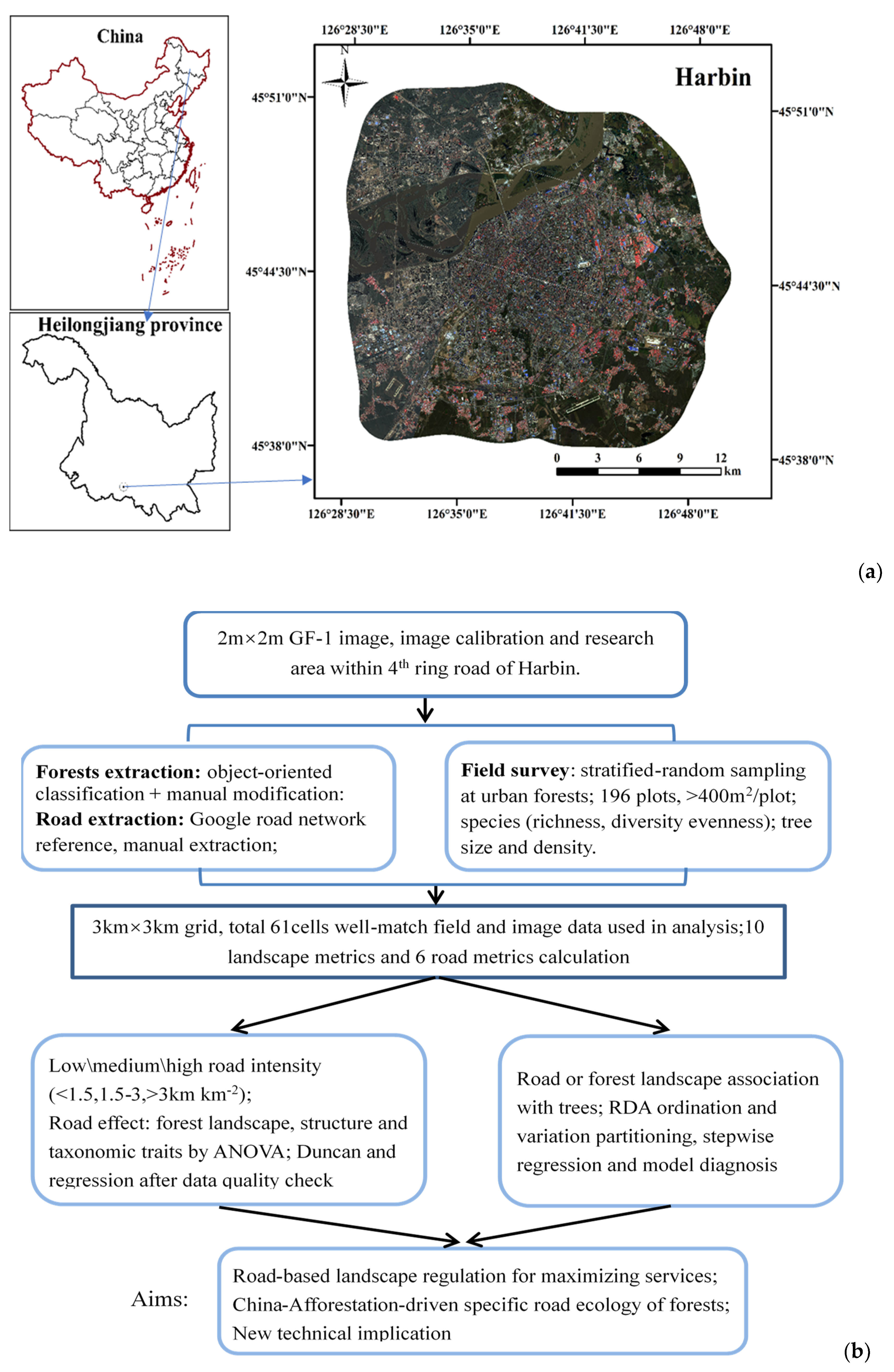
2.1. Study Area
2.2. Road Density Identification and Road-Related Traits Computation
2.3. Urban Forest Characteristics Survey: Structural-Taxonomic Attributes
2.4. Analysis of Urban Forest Landscape Patterns
2.5. Statistical Analysis
3. Results
3.1. Characterization of the Study Object in Road Characteristics
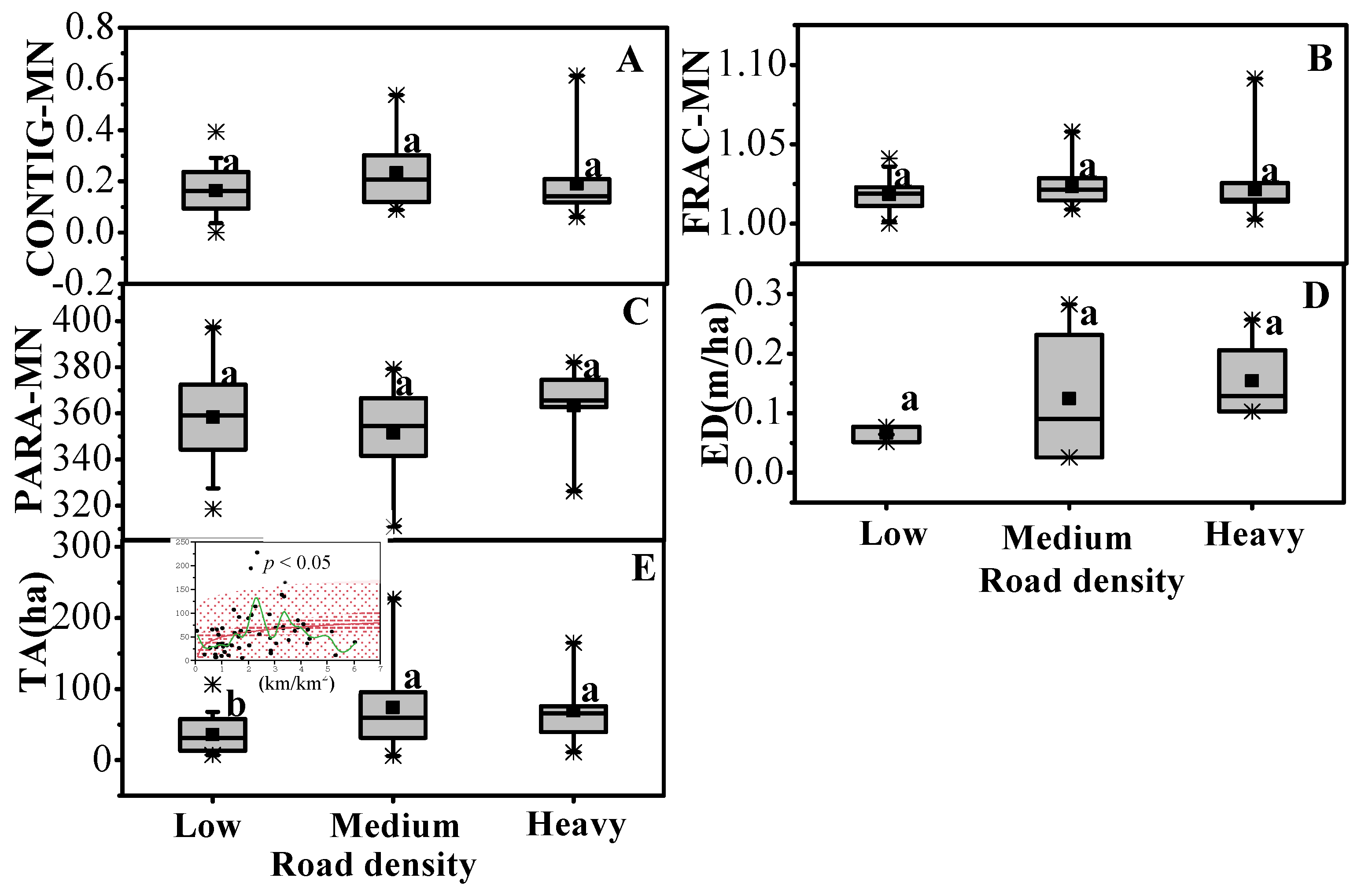
3.2. Landscape Metrics of Urban Forests
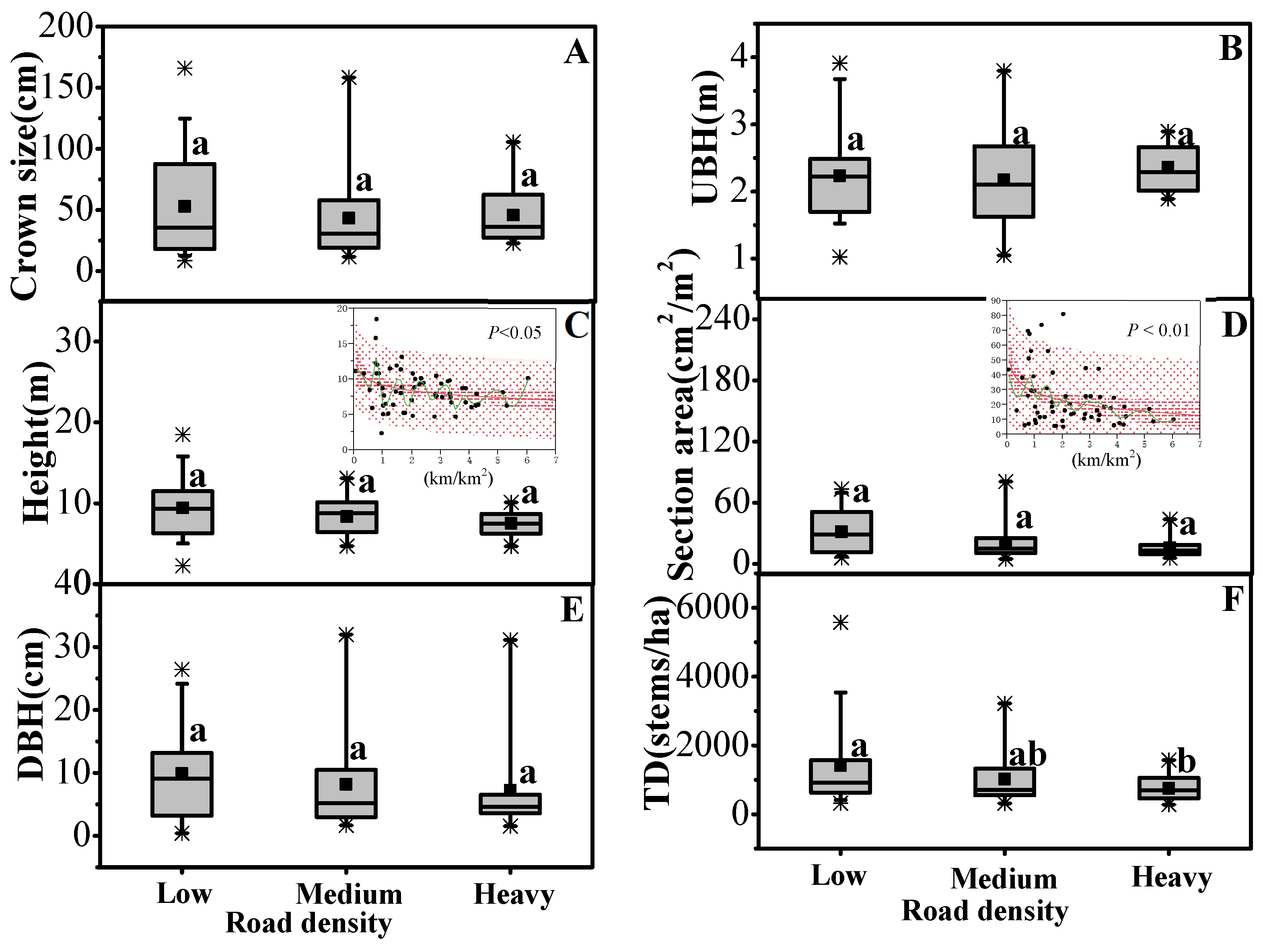
3.3. Structural and Taxonomic Attributes of Urban Trees
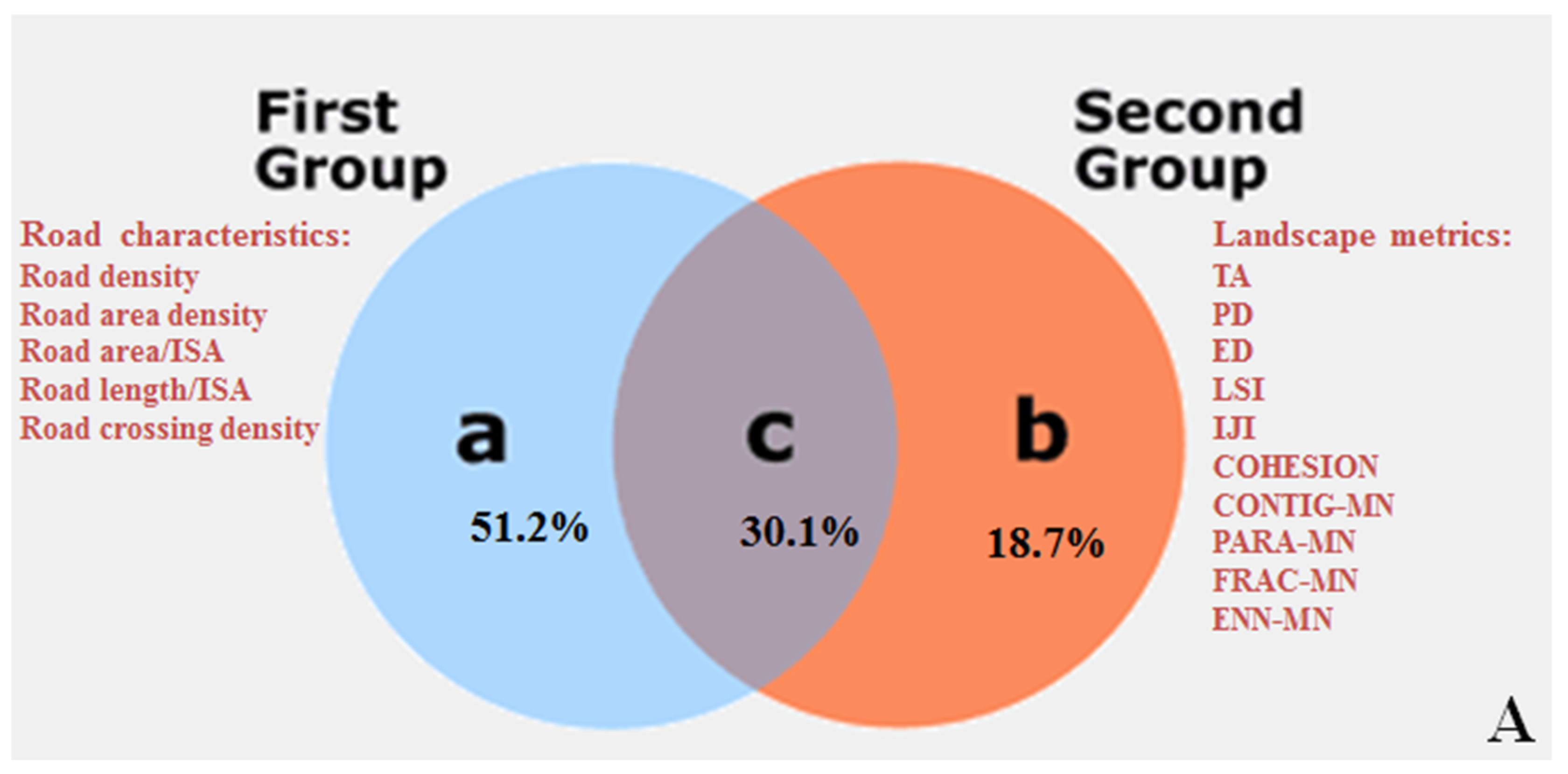
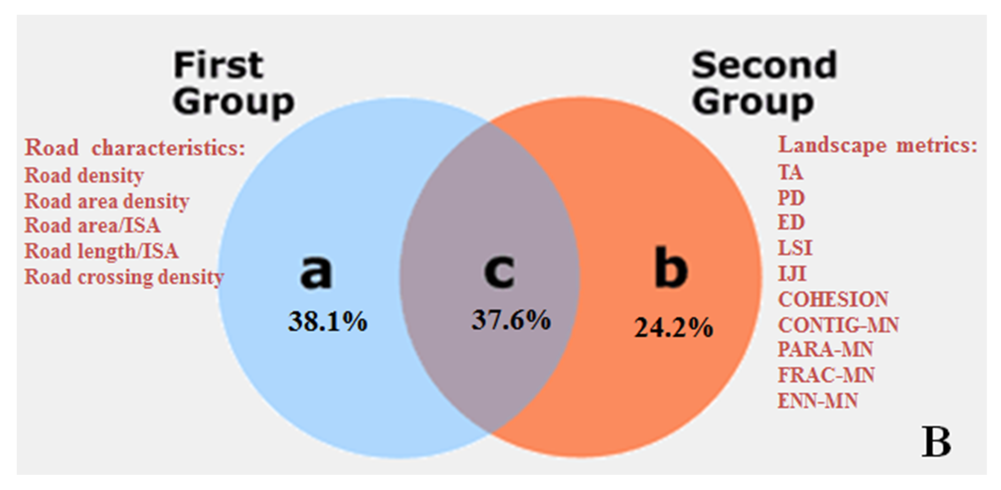
3.4. Association Decoupling
3.5. Significant Parameters that Explain Forest Variation
4. Discussion
4.1. Road Development Associated with Increased Forest Areas Characterized by More Patches, Complex Shapes, Smaller Tree Sizes, Lower Density, and More Diversified Species Compositions
4.2. Road-Dependent Landscape Regulation Could Improve Forest Ecological Services
4.3. Technical Implications and Uncertainty
5. Conclusions
Supplementary Materials
Author Contributions
Acknowledgments
Conflicts of Interest
References
- Li, Y.; Hu, Y.; Li, X.; Xiao, D. A review on road ecology. Chin. J. Appl. Ecol. 2003, 14, 447–452. [Google Scholar]
- Alexander, L.E. Roads and their major ecological effects. Annu. Rev. Ecol. Syst. 1998, 29, 207–231. [Google Scholar]
- Liu, S.; Yang, Z.; Cui, B.; Gan, S. Effects of road on landscape and its ecological risk assessment: A case study of Lancangjiang river valley. Chin. J. Ecol. 2005, 24, 897–901. [Google Scholar]
- Cai, X.; Wu, Z.; Cheng, J. Using kernel density estimation to assess the spatial pattern of road density and its impact on landscape fragmentation. Int. J. Geogr. Inf. Sci. 2013, 27, 222–230. [Google Scholar] [CrossRef]
- Wang, J.; Cui, B.; Liu, S.; Liu, J. Effects of different level road networks on landscape structure health in the longitudinal range-gorge region. Acta Sci. Circumstantiae 2008, 28, 261–268. [Google Scholar]
- Coffin, A. From roadkill to road ecology: A review of the ecological effects of roads. J. Transp. Geogr. 2007, 15, 396–406. [Google Scholar] [CrossRef]
- Ree, R.V.D.; Smith, D.J.; Grilo, C. Handbook of Road Ecology; John Wiley & Sons: Hoboken, NJ, USA, 2015; pp. 1–9. [Google Scholar]
- Cao, W.; Luo, F.; Han, J.; Caiyan, W.U.; Xiang, W. The impact of road development on landscape pattern change in rapidly urbanizing area. J. Geo-Inf. Sci. 2014, 16, 898–906. [Google Scholar]
- Huang, R.; Ma, Y.-X.; Li, H.-M.; Liu, W.J. Effect of road development on landscape pattern in Xishuangbanna. J. Yunnan Univ. 2013, 35, 121–128. [Google Scholar]
- Li, S.; Xu, Y.; Zhou, Q.; Wang, L. Statistical analysis on the relationship between road network and ecosystem fragmentation in China. Prog. Geogr. 2004, 23, 78–85. [Google Scholar]
- Peng, Z. Forest networking and waterchannel networking—China urban forest construction idea. China Urban For. 2003, 1, 4–12. [Google Scholar]
- Livesley, S.J.; Mcpherson, G.M.; Calfapietra, C. The urban forest and ecosystem services: Impacts on urban water, heat, and pollution cycles at the tree, street, and city scale. J. Environ. Qual. 2016, 45, 119–124. [Google Scholar] [CrossRef] [PubMed]
- Zhai, C.; Wang, W.; He, X.; Zhou, W.; Xiao, L.; Zhang, B. Urbanization drives soc accumulation, its temperature stability and turnover in forests, northeastern China. Forests 2017, 8, 130. [Google Scholar] [CrossRef]
- Zhang, B.; Wang, W.; He, X.; Zhou, W.; Xiao, L.; Lv, H.; Wei, C. Shading, cooling and humidifying effects of urban forests in harbin city and possible association with various factors. Chin. J. Ecol. 2017, 36, 951–961. [Google Scholar]
- Lv, H.; Wang, W.; He, X.; Xiao, L.; Zhou, W.; Zhang, B. Quantifying tree and soil carbon stocks in a temperate urban forest in northeast China. Forests 2016, 7, 200. [Google Scholar] [CrossRef]
- Liu, S.L.; Cui, B.S.; Dong, S.K.; Yang, Z.F.; Yang, M.; Holt, K. Evaluating the influence of road networks on landscape and regional ecological risk—A case study in lancang river valley of southwest China. Ecol. Eng. 2008, 34, 91–99. [Google Scholar] [CrossRef]
- Li, Y.-H.; Wu, Z.-F.; Chen, H.W.; Li, N.-N.; Hu, Y.-M.; Chang, Y. Impacts of road network on forest landscape pattern in great Xing’an mountains of northeast China. Chin. J. Appl. Ecol. 2012, 23, 2087–2092. [Google Scholar]
- He, X.; Ren, Z.; Zheng, H.; Wang, W. Urban forest research in China: Review and perspective. In Urban Forest Sustainability; Ning, Z., Novak, D., Watson, G., Eds.; International Society of Arboriculture: Champaign, IL, USA, 2017; pp. 12–37. [Google Scholar]
- Etheridge, D.A.; MacLean, D.A.; Wagner, R.G.; Wilson, J.S. Effects of intensive forest management on stand and landscape characteristics in northern New Brunswick, Canada (1945–2027). Landsc. Ecol. 2006, 21, 509–524. [Google Scholar] [CrossRef]
- Ribeiro, S.C.; Lovett, A. Associations between forest characteristics and socio-economic development: A case study from Portugal. J. Environ. Manag. 2009, 90, 2873–2881. [Google Scholar] [CrossRef]
- Sano, M.; Miyamoto, A.; Furuya, N.; Kogi, K. Using landscape metrics and topographic analysis to examine forest management in a mixed forest, Hokkaido, Japan: Guidelines for management interventions and evaluation of cover changes. For. Ecol. Manag. 2009, 257, 1208–1218. [Google Scholar] [CrossRef]
- Uuemaa, E.; Mander, Ü.; Marja, R. Trends in the use of landscape spatial metrics as landscape indicators: A review. Ecol. Indic. 2013, 28, 100–106. [Google Scholar] [CrossRef]
- Wang, W.; Wang, Q.; Zhou, W.; Xiao, L.; Wang, H.; He, X. Glomalin changes in urban-rural gradients and their possible associations with forest characteristics and soil properties in Harbin city, northeastern China. J. Environ. Manag. 2018, 224, 225–234. [Google Scholar] [CrossRef] [PubMed]
- Zhang, D.; Wang, W.; Zheng, H.; Ren, Z.; Zhai, C.; Tang, Z.; Shen, G.; He, X. Effects of urbanization intensity on forest structural-taxonomic attributes, landscape patterns and their associations in Changchun, northeast China: Implications for urban green infrastructure planning. Ecol. Indic. 2017, 80, 286–296. [Google Scholar] [CrossRef]
- Wang, X.-J. Analysis of problems in urban green space system planning in China. J. For. Res. 2009, 20, 79–82. [Google Scholar] [CrossRef]
- Pan, L.; Zhang, H.; Liu, A. Analysis of threshold of road networks effecting landscape fragmentation in Chongqing. Ecol. Sci. 2015, 34, 45–51. [Google Scholar]
- Wang, L.; Zeng, H. The principle of road network structures and its ecological effects on landscape in Shenzhen. Geogr. Res. 2012, 31, 853–862. [Google Scholar]
- Wang, W.; Wang, H.; Xiao, L.; He, X.; Zhou, W.; Wang, Q.; Wei, C. Microclimate regulating functions of urban forests in Changchun city (north-east China) and their associations with different factors. iFor.-Biogeosci. For. 2018, 11, 140–147. [Google Scholar] [CrossRef]
- Zhang, J.; Wang, W.; Du, H.; Zhong, Z.; Xiao, L.; Zhou, W.; Zhang, B.; Wang, H. Differences in community characteristics, species diversity, and their coupling associations among three forest types in the Huzhong area, Daxinganling mts. Acta Ecol. Sin. 2018, 38, 4684–4693. [Google Scholar]
- Zhong, Z.; Wang, W.; Wang, Q.; Wu, Y.; Wang, H.; Pei, Z. Glomalin amount and compositional variation, and their associations with soil properties in farmland, northeastern China. J. Plant Nutr. Soil Sci. 2017, 180, 563–575. [Google Scholar] [CrossRef]
- Lv, H.; Wang, W.; He, X.; Wei, C.; Xiao, L.; Zhang, B.; Zhou, W. Association of urban forest landscape characteristics with biomass and soil carbon stocks in Harbin city, northeastern China. PeerJ 2018, 6, e5825. [Google Scholar] [CrossRef]
- Xiao, L.; Wang, W.; He, X.; Lv, H.; Wei, C.; Zhou, W.; Zhang, B. Urban-rural and temporal differences of woody plants and bird species in Harbin city, northeastern China. Urban For. Urban Green. 2016, 20, 20–31. [Google Scholar] [CrossRef]
- Wu, Y.; Wang, W. Poplar forests in NE China and possible influences on soil properties: Ecological importance and sustainable development. In Poplars & Willows, Cultivation, Applications & Environmental Benefits; Desmond, M., Ed.; Novapublishers: Hauppauge, NY, USA, 2016; pp. 1–28. [Google Scholar]
- Wang, W. Harbin Urban Forest Characteristics and Ecological Service Functions; Science Press: Beijing, China, 2019; p. 207. [Google Scholar]
- Qin, Y. Study in Harbin: The development and tendency of population growth. J. Nanjing Coll. Popul. Programme Manag. 2006, 22, 5–8. [Google Scholar]
- Zheng, W.; Zhou, Y.; Gu, H.; Tian, Z. Seasonal dynamics and impact factors of urban forest CO2 concentration in Harbin, China. J. For. Res. 2017, 28, 125–132. [Google Scholar] [CrossRef]
- Ren, Z.; Du, Y.; He, X.; Pu, R.; Zheng, H.; Hu, H. Spatiotemporal pattern of urban forest leaf area index in response to rapid urbanization and urban greening. J. For. Res. 2018, 29, 785–796. [Google Scholar] [CrossRef]
- Dai, L.; Li, S.; Lewis, B.J.; Wu, J.; Yu, D.; Zhou, W.; Zhou, L.; Wu, S. The influence of land use change on the spatial–temporal variability of habitat quality between 1990 and 2010 in northeast China. J. For. Res. 2018. [Google Scholar] [CrossRef]
- Cui, L.; Mu, L. Ectomycorrhizal communities associated with tilia amurensis trees in natural versus urban forests of Heilongjiang in northeast China. J. For. Res. 2016, 27, 401–406. [Google Scholar] [CrossRef]
- Zhou, W.; Wang, W.; He, X.; Zhang, B.; Xiao, L.; Wang, Q.; Lv, H.; Wei, C. Soil fertility and its spatial heterogeneity of urban green land in Harbin, NE China. Sci. Silvae Sin. 2018, 54, 9–17. [Google Scholar]
- Xiao, L.; Wang, W.; Zhang, D.; He, X.; Wei, C.; Lv, H.; Zhou, W.; Zhang, B. Urban forest tree species composition and arrangement reasonability in Harbin, northeast China. Chin. J. Ecol. 2016, 35, 2074–2081. [Google Scholar]
- Wang, W.; Zhang, B.; Xiao, L.; Zhou, W.; Wang, H.; He, X. Decoupling forest characteristics and background conditions to explain urban-rural variations of multiple microclimate regulation from urban trees. PeerJ 2018, 6, e5450. [Google Scholar] [CrossRef]
- Wang, W.; Xiao, L.; Zhang, J.; Yang, Y.; Tian, P.; Wang, H.; He, X. Potential of internet street-view images for measuring tree sizes in roadside forests. Urban For. Urban Green. 2018, 35, 211–220. [Google Scholar] [CrossRef]
- Hawbaker, T.J.; Radeloff, V.C.; Hammer, R.B.; Clayton, M.K. Road density and landscape pattern in relation to housing density, and ownership, land cover, and soils. Landsc. Ecol. 2005, 20, 609–625. [Google Scholar] [CrossRef]
- Shannon, C.E. The mathematical theory of communication. 1963. M.D. Comput. Comput. Med. Pract. 1997, 14, 306–317. [Google Scholar]
- Magurran, A.E. Ecological Diversity and Its Measurement; Princeton University Press: Princeton, NJ, USA, 1988; pp. 81–99. [Google Scholar]
- Pielou, E.C. The measurement of diversity in different types of biological collections. J. Theor. Biol. 1966, 13, 131–144. [Google Scholar] [CrossRef]
- Fahey, R.T.; Casali, M. Distribution of forest ecosystems over two centuries in a highly urbanized landscape. Landsc. Urban Plan. 2017, 164, 13–24. [Google Scholar] [CrossRef]
- Zhang, J.; Sta, P. Effects of urbanization on forest vegetation, soils and landscape. Acta Ecol. Sin. 1999, 19, 654–658. [Google Scholar]
- Tuffery, L. The recreational services value of the nearby periurban forest versus the regional forest environment. J. For. Econ. 2017, 28, 33–41. [Google Scholar] [CrossRef]
- Jim, C.Y.; Zhang, H. Species diversity and spatial differentiation of old-valuable trees in urban Hong Kong. Urban For. Urban Green. 2013, 12, 171–182. [Google Scholar] [CrossRef]
- Riley, C.B.; Herms, D.A.; Gardiner, M.M. Exotic trees contribute to urban forest diversity and ecosystem services in inner-city Cleveland, OH. Urban For. Urban Green. 2017, 29, 367–376. [Google Scholar] [CrossRef]
- Jokimäki, J.; Suhonen, J.; Inki, K.; Jokinen, S. Biogeographical comparison of winter bird assemblages in urban environments in Finland. J. Biogeogr. 1996, 23, 379–386. [Google Scholar] [CrossRef]
- Morelli, F.; Benedetti, Y.; Ibáñez-Álamo, J.D.; Jokimäki, J.; Mänd, R.; Tryjanowski, P.; Møller, A.P. Evidence of evolutionary homogenization of bird communities in urban environments across Europe. Glob. Ecol. Biogeogr. 2016, 25, 1284–1293. [Google Scholar] [CrossRef]
- Schmidt, K.J.; Poppendieck, H.H.; Kai, J. Effects of urban structure on plant species richness in a large European city. Urban Ecosyst. 2014, 17, 427–444. [Google Scholar] [CrossRef]
- Wang, H.F.; Qureshi, S.; Qureshi, B.A.; Qiu, J.X.; Friedman, C.R.; Breuste, J.; Wang, X.K. A multivariate analysis integrating ecological, socioeconomic and physical characteristics to investigate urban forest cover and plant diversity in Beijing, China. Ecol. Indic. 2016, 60, 921–929. [Google Scholar] [CrossRef]
- Lindenmayer, D.B.; Franklin, J.F.; Fischer, J. General management principles and a checklist of strategies to guide forest biodiversity conservation. Biol. Conserv. 2006, 131, 433–445. [Google Scholar] [CrossRef]
- Kuuluvainen, T. Forest management and biodiversity conservation based on natural ecosystem dynamics in northern Europe: The complexity challenge. Ambio 2009, 38, 309–315. [Google Scholar] [CrossRef] [PubMed]
- Groffman, P.M.; Cavender-Bares, J.; Bettez, N.D.; Grove, J.M.; Hall, S.J.; Heffernan, J.B.; Hobbie, S.E.; Larson, K.L.; Morse, J.L.; Neill, C. Ecological homogenization of urban USA. Front. Ecol. Environ. 2014, 12, 74–81. [Google Scholar] [CrossRef]
- Liu, S.L.; Wen, M.X.; Cui, B.S.; Dong, S.K. Effects of road networks on regional ecosystems in southwest mountain area:A case study in Jinhong of longitudinal range-gorge region. Acta Ecol. Sin. 2006, 26, 3018–3024. [Google Scholar]
- Bailey, D.; Herzog, F.; Augenstein, I.; Aviron, S.; Billeter, R.; Szerencsits, E.; Baudry, J. Thematic resolution matters: Indicators of landscape pattern for European agro-ecosystems. Ecol. Indic. 2007, 7, 692–709. [Google Scholar] [CrossRef]
- Albert, C.; Galler, C.; Hermes, J.; Neuendorf, F.; Haaren, C.V.; Lovett, A. Applying ecosystem services indicators in landscape planning and management: The es-in-planning framework. Ecol. Indic. 2015, 61, 100–113. [Google Scholar] [CrossRef]
- Nowak, D.J.; Crane, D.E. Carbon storage and sequestration by urban trees in the USA. Environ. Pollut. 2002, 116, 381–389. [Google Scholar] [CrossRef]
- Ren, Z.; Zheng, H.; He, X.; Zhang, D.; Yu, X.; Shen, G. Spatial estimation of urban forest structures with landsat tm data and field measurements. Urban For. Urban Green. 2015, 14, 336–344. [Google Scholar] [CrossRef]
- Lanza, K.; Stone, B., Jr. Climate adaptation in cities: What trees are suitable for urban heat management? Landsc. Urban Plan. 2016, 153, 74–82. [Google Scholar] [CrossRef]
- Inkiläinen, E.N.M.; Mchale, M.R.; Blank, G.B.; James, A.L.; Nikinmaa, E. The role of the residential urban forest in regulating throughfall: A case study in Raleigh, North Carolina, USA. Landsc. Urban Plan. 2013, 119, 91–103. [Google Scholar] [CrossRef]
- Hernandez-Stefanoni, J.L. The role of landscape patterns of habitat types on plant species diversity of a tropical forest in Mexico. Biodivers. Conserv. 2006, 15, 1441–1457. [Google Scholar] [CrossRef]
- Dobbs, C.; Kendal, D.; Nitschke, C.R. Multiple ecosystem services and disservices of the urban forest establishing their connections with landscape structure and sociodemographics. Ecol. Indic. 2014, 43, 44–55. [Google Scholar] [CrossRef]
- Schindler, S.; Wehrden, H.V.; Poirazidis, K.; Wrbka, T.; Kati, V. Multiscale performance of landscape metrics as indicators of species richness of plants, insects and vertebrates. Ecol. Indic. 2013, 31, 41–48. [Google Scholar] [CrossRef]
- Wu, Y.; Wang, W.; Wang, Q.; Zhong, Z.; Pei, Z.; Wang, H.; Yao, Y. Impact of poplar shelterbelt plantations on surface soil properties in northeast China. Can. J. For. Res. 2018, 48, 559–567. [Google Scholar] [CrossRef]
- Wang, W.; Zhong, Z.; Wang, Q.; Wang, H.; Fu, Y.; He, X. Glomalin contributed more to carbon, nutrients in deeper soils, and differently associated with climates and soil properties in vertical profiles. Sci. Rep. 2017, 7, e13003. [Google Scholar] [CrossRef]
- Eisenhauer, N.; Bowker, M.A.; Grace, J.B.; Powell, J.R. From patterns to causal understanding: Structural equation modeling (SEM) in soil ecology. Pedobiologia 2015, 58, 65–72. [Google Scholar] [CrossRef]
- Ma, K. Forest dynamics plot is a crosscutting research platform for biodiversity science. Biodivers. Sci. 2017, 25, 227–228. [Google Scholar] [CrossRef]
- Wang, W.J.; Qiu, L.; Zu, Y.G.; Su, D.X.; An, J.; Wang, H.Y.; Zheng, G.Y.; Sun, W.; Chen, X.Q. Changes in soil organic carbon, nitrogen, pH and bulk density with the development of larch (Larix gmelinii) plantations in China. Glob. Chang. Biol. 2011, 17, 2657–2676. [Google Scholar]
- Wang, C.; Peng, Z.; Tao, K. Characteristic and development of urban forest in China. Chin. J. Ecol. 2004, 23, 88–92. [Google Scholar]


| Metrics | Calculation and Range | Description |
|---|---|---|
| Total Area (TA) | TA equals the total area (m2) of the landscape, divided by 10,000 (to convert to hectares). | |
| Edge Density (ED) | ED equals the sum of the lengths (m) of all edge segments in the landscape, divided by the total landscape area (m2), and multiplied by 10,000 (to convert to hectares). | |
| Patch Density (PD) | PD equals the number of patches in the landscape, divided by total landscape area (m2), and multiplied by 10,000 and 100 (to convert to 100 hectares). PD is one of the most important indices to describe landscape heterogeneity. | |
| Landscape Shape Index (LSI) | LSI equals 0.25 (adjustment for raster format) times the sum of the landscape boundary and all edge segments (m) within the landscape boundary and divided by the square root of the total landscape area (m2). LSI measures the aggregation of patches. A large LSI value indicates a more irregular landscape. | |
| Mean Fractal Dimension Index (FRAC-MN) | FRAC-MN equals the mean value of the sum of 2 times the logarithm of the patch perimeter (m) divided by the logarithm of the patch area (m2) for each patch of the corresponding landscape. It reflects shape complexity. FRAC approaches 1 for shapes with very simple perimeters such as squares and approaches 2 for shapes with highly convoluted, plane-filling perimeters. | |
| Mean Perimeter Area Ratio (PARA-MN) | PARA-MN equals the mean value of the ratio of the patch perimeter (m) to area (m2), and PARA is a simple measure of shape complexity. | |
| Mean Contiguity Index (CONTIG_MN) | CONTIG equals the average contiguity value for the cells in a patch (i.e., sum of the cell values divided by the total number of pixels in the patch) minus 1 and divided by the sum of the template values (13 in this case) minus 1. The contiguity index assesses the spatial connectedness, or contiguity, of cells within a grid-cell patch to provide an index on the patch boundary configuration and thus the patch shape. | |
| Mean Euclidian Nearest Neighbor Distance (ENN_MN) | ENN_MN is the mean value of the distance (m) to the nearest neighboring patch of the landscape, based on the shortest edge-to-edge distance. Note that the edge-to-edge distances are from cell center to cell center. ENN_MN measures the isolation of the patches of the landscape. The straight line distance is the shortest path between the patches. | |
| Interspersion and Juxtaposition Index (IJI) | IJI equals a negative sum of the length (m) of each unique edge type divided by the total landscape edge (m), multiplied by the logarithm of the same quantity, and summed over each unique edge type; divided by the logarithm of the number of patch types, times the number of patch types, minus 1, and divided by 2; and multiplied by 100 (to convert to a percentage). IJI provides a measure of isolating the interspersion or intermixing of patch types. | |
| Patch Cohesion Index (COHESION) | COHESION equals 1 minus the sum of the patch perimeter (in terms of number of cells), divided by the sum of the patch perimeter, times the square root of the patch area (in terms of number of cells) for all patches in the landscape, divided by 1 minus 1 over the square root of the total number of cells in the landscape, and multiplied by 100 to convert to a percentage. The patch cohesion increases as the patch type becomes more clumped or aggregated in its distribution. |
| Parameters (y) | Statistical Index | Road Intensity Regions | Liner Regression from Low to Heavy RD | ||||
|---|---|---|---|---|---|---|---|
| Low RD | Medium RD | Heavy RD | Equation | R2 | p Value | ||
| RD (km/km2) | mean value | 0.92 | 2.16 | 3.96 | y = 1.5097x − 0.6714 | 0.8288 | <0.01 |
| standard error | 0.07 | 0.10 | 0.20 | ||||
| Significance | c | b | a | ||||
| RAD (km2/km2) | mean value | 0.019 | 0.058 | 0.12 | y = 0.049x − 0.0328 | 0.7289 | <0.01 |
| standard error | 0.0023 | 0.0052 | 0.0086 | ||||
| Significance | c | b | a | ||||
| RAI (km2/km2) | mean value | 0.043 | 0.14 | 0.32 | y = 0.136x − 0.1027 | 0.3915 | <0.01 |
| standard error | 0.0058 | 0.028 | 0.053 | ||||
| Significance | c | b | a | ||||
| RLI (km/km2) | mean value | 4.97 | 11.09 | 21.8 | y = 8.357x − 4.0384 | 0.2964 | <0.01 |
| standard error | 0.89 | 2.67 | 3.61 | ||||
| Significance | c | b | a | ||||
| CPD (point/km2) | mean value | 0.54 | 1.94 | 4.73 | y = 2.1876x − 1.9159 | 0.6905 | <0.01 |
| standard error | 0.091 | 0.23 | 0.51 | ||||
| Significance | c | b | a | ||||
| ISA (%) | mean value | 53.0 | 55.8 | 52.5 | y = −0.165x + 54.044 | 0.00003 | >0.05 |
| standard error | 5.8 | 6.5 | 6.5 | ||||
| Significance | a | a | a | ||||
| Y Items | Equations with RDs as X (km/1000 m2) | Logarithmic Slope or Exponent | R2 | p-Value |
|---|---|---|---|---|
| Landscape metrics | ||||
| PD (no./grid) | y = 0.1379ln(x) + 0.5146 | 0.1379 | 0.134 | p < 0.01 |
| TA (ha/grid) | y = 15.5 × l n(x) + 50.2 | 15.5 | 0.073 | p < 0.05 |
| LSI | y = 0.7415ln(x) + 4.7194 | 0.7415 | 0.1501 | p < 0.01 |
| Structural attributes | ||||
| Height (m) | y = −1.10ln(x) + 9.171 | −1.10 | 0.094 | p < 0.05 |
| Section area (cm2/m2) | y = −8.137ln(x) + 28.59 | −8.137 | 0.1160 | p < 0.01 |
| Taxonomic attributes | ||||
| SR | y = 2.0703ln(x) + 5.217 | 2.0703 | 0.135329 | p < 0.01 |
| H’ | y = 0.3196 × ln(x) + 0.7097 | 0.3196 | 0.1866 | p < 0.001 |
| J’ | y = 0.1117ln(x) + 0.4083 | 0.1117 | 0.1228 | p < 0.01 |
| Region | Dependent Variables | Final Model | R2 | p-Value |
|---|---|---|---|---|
| Low RD | Height | 13.011 − 0.273(IJI) − 153.038(RAD) | 0.434 | 0.004 |
| Section area | −2079 − 1.26(IJI) + 2002(FRAC_MN) − 565(ED) − 343(RAI) + 0.32(PARA_MN) − 9.67(CPD) | 0.865 | 0.000 | |
| DBH | 14.12 − 0.12(TA) | 0.16 | 0.067 | |
| Tree density | 549 + 1659(CPD) | 0.325 | 0.006 | |
| UBH | 3.43 − 0.003(ENN_MN) − 9.06(ED) | 0.281 | 0.044 | |
| Canopy size | 133 + 6.72(RLI) − 0.20(ENN_MN) − 39.40(CPD) − 604(ED) | 0.672 | 0.000 | |
| H’ | −0.04 + 36.13(RAD) | 0.432 | 0.001 | |
| SR | −0.07 + 243(RAD) | 0.472 | 0.000 | |
| Medium and heavy RDs | Tree height | 9.59 − 0.0047(ENN-MN) | 0.084 | 0.088 |
| Section area | 27.3 − 96.3(RAD) | 0.078 | 0.099 | |
| DBH | −52.6 + 0.19(PARA_MN) − 2.28(RLD) | 0.191 | 0.030 | |
| Tree density | 1655 − 105.1(CPD) − 7.34(ISA%) | 0.189 | 0.032 | |
| UBH | 1.27 + 0.018(COHESION) + 5.04(RAD) − 2.77(ED) | 0.289 | 0.011 | |
| Canopy size | 24.4 + 0.39(ISA%) | 0.123 | 0.037 | |
| H’ | 0.75 + 0.021(IJI) + 0.01(RLI) | 0.187 | 0.033 | |
| SR | 1.61 + 1.03(LSI) | 0.102 | 0.059 |
© 2019 by the authors. Licensee MDPI, Basel, Switzerland. This article is an open access article distributed under the terms and conditions of the Creative Commons Attribution (CC BY) license (http://creativecommons.org/licenses/by/4.0/).
Share and Cite
Yang, Y.; Lv, H.; Fu, Y.; He, X.; Wang, W. Associations between Road Density, Urban Forest Landscapes, and Structural-Taxonomic Attributes in Northeastern China: Decoupling and Implications. Forests 2019, 10, 58. https://doi.org/10.3390/f10010058
Yang Y, Lv H, Fu Y, He X, Wang W. Associations between Road Density, Urban Forest Landscapes, and Structural-Taxonomic Attributes in Northeastern China: Decoupling and Implications. Forests. 2019; 10(1):58. https://doi.org/10.3390/f10010058
Chicago/Turabian StyleYang, Yanbo, Hailiang Lv, Yujie Fu, Xingyuan He, and Wenjie Wang. 2019. "Associations between Road Density, Urban Forest Landscapes, and Structural-Taxonomic Attributes in Northeastern China: Decoupling and Implications" Forests 10, no. 1: 58. https://doi.org/10.3390/f10010058
APA StyleYang, Y., Lv, H., Fu, Y., He, X., & Wang, W. (2019). Associations between Road Density, Urban Forest Landscapes, and Structural-Taxonomic Attributes in Northeastern China: Decoupling and Implications. Forests, 10(1), 58. https://doi.org/10.3390/f10010058