Article

A Novel Comprehensive Evaluation Method of Forest State Based on Unit Circle

Key Laboratory of Tree Breeding and Cultivation of State Forestry Administration, Research Institute of Forestry, Chinese Academy of Forestry, Beijing 100091, China
*
Author to whom correspondence should be addressed.
Forests 2019, 10(1), 5; https://doi.org/10.3390/f10010005
Submission received: 18 November 2018 / Revised: 15 December 2018 / Accepted: 18 December 2018 / Published: 21 December 2018
(This article belongs to the Section Forest Ecology and Management)

Abstract

:
Comprehensive evaluation of forest state is the precondition and critical step for forest management. To solve the problem that the radar plot and unit circle only focus on the value of each the evaluation index, this paper proposes a novel method for comprehensively and simultaneously evaluating the functionality and inhomogeneity of forest state based on the modified unit circle method. We evaluated the forest state of the Quercus aliena BL. var. acuteserrata Maxim. ex Wenz. broad-leaved mixed forest in the Xiaolong Mountains Forest Area of Gansu Province and the Pinus koraiensis Sieb. et Zucc. broad-leaved mixed forest in Jilin Province in China. According to the principle of comprehensive, scientific and operability, 10 evaluation indices on forest structure and vitality were selected to construct the evaluation indicator system. Each index was normalized based on the assignment method and ensured to be strictly positive based on reciprocal transformation method. The areas and arc length of the closed graph, formed by connecting every two adjacent indicators, in the radar plot and unit circle were extracted. Based on the isoperimetric theorem (isoperimetric inequality), a comprehensive evaluation model was constructed. Compared with radar chart and unit circle method, each index in the newly proposed unit circle method is represented by an independent sector region, reflecting the contribution of the index to the overall evaluation result. Each index has the same relative importance weight, contributing to the estimation the relative sizes of each aspect of forest state. The unique area and arc length of the closed graph help summarize the overall performance with a global score. The expression effect of improved unit circle has been enhanced, and as an English proverb put it, “A picture is worth a thousand words.” The new proposed method simultaneously evaluates the functionality and inhomogeneity of the forest state and it is a powerful tool for the diagnosis of forest state problems and the decision-making of forest management.

1. Introduction

Forest state is the state and properties of a stand of trees in natural habitats [1]. It is the specific expression of forest condition at present and the basic of the growth potential and development direction in the future. Forest state is directly related to the necessity and urgency of forest management. Forest state evaluation is the precondition of forest management activities, the core task of evaluation and decision-making are the “measures” and “choice”, respectively [2]. Therefore, constructing a scientific index system and choosing a reasonable method for evaluation are the key prerequisite factors to compare different forest states and establish supporting management measures. Many researches have been completed based on forest state characteristics, for example, the method of forest experimental design [3], the method of forest naturalness assessment [4], the π value rule of forest optimal stand state [1] and the priority of management measures for natural forests [5]. In the past, the description of forest state was simply expressed in words and tables [6], leading to the phenomenon of “data rich but information poor” [7], demonstrating the need for objective, concise and effective evaluation of the forest state, and multi-dimensional evaluation information should be intuitively displayed in a simple and practical form.
Comprehensive evaluation, referring to making global and integrality description of multiple attribute evaluation object, should not only consider the functionality of evaluation indicators, that is, the value of each evaluation index but also the inhomogeneity among the evaluation indicators by emphasizing the inhomogeneity of evaluation indices [8]. Of the various comprehensive evaluation methods, radar graph analysis method is a visualized multi-attribute comprehensive evaluation method that intuitively displays the relative superiority of the evaluation object in various indicators and make overall evaluation at the same time. It has the characteristics of simplicity, intuition, and strong operability [9,10,11,12], and has been widely used in forestry and environment studies [5,13,14,15,16,17,18,19,20,21]. However, the radar plot used in these studies has one fatal defect—the non-uniqueness of feature vector area and perimeter caused by different ranking order of evaluation indicators [12]. Hui et al. [1] adopted the index ranking method to obtain a relatively unique area eigenvalue, and proposed unit circle method to evaluate the natural forest state using the overall area of the closed graph in unit circle. The radar plot and unit circle method only focus on the final score of different evaluation objects and do not reflect the inhomogeneity among the attributes of these objects.
According to the Leaky Bucket Theory and Liebig’s Law of the Minimum [22], that is, the performance of an evaluation system mainly depends on its minimum index value. If the indicators of two evaluation objects take values of (1, 2, 3) and (2, 2, 2), then the former object has a relatively weaker score than the latter although they have the same total scores [23]. Thus, the quantitative inhomogeneity among multiple attributes of evaluation objects can influence the overall assessment of the study subjects [23]. The radar plot and unit circle method calculate the area characteristics value according to every two adjacent indices, ignoring the independence of the individual indicators and its contribution to the overall. In either method, the value of an index, especially if it equals to zero, has a considerable influence on the overall result and the final results only highlight the functionality of the evaluation system. These shortcuts may lead to the unbalance development [8], instead of the comprehensive and sustainable development.
This article takes as examples a forest state evaluation of the Quercus aliena BL. var. acuteserrata Maxim. ex Wenz. broad-leaved mixed forest in the Xiaolong Mountains Forest Region of Gansu Province and the P. koraiensis Sieb. et Zucc. broad-leaved mixed forest in Jilin Province in China. The objectives of this article were: (1) to propose a new comprehensive evaluation method to analyze the functionality and inhomogeneity of forest state simultaneously; (2) to verify the effectiveness and superiority of the newly proposed methods by comparative analysis with the radar plot, unit circle, and modified unit circle; and (3) to explore the potential problems of the forest state and the implication for the decision-making of forest management.

2. Materials and Methods

2.1. Study Region and Sampling Plot

2.1.1. Study Region

Xiaolong Mountains Forest Region (104°22′–106°43′ E, 33°30′–34°49′ N) is located in the southeast of Gansu province and western part of Qinling mountains (Figure 1a). It is a transitional zone from warm temperate to a northern subtropical climate, with climate characteristics of both north and south China. Most areas experience warm humid–temperate semi humid continental monsoon climate. The altitude is between 1000 m and 2000 m a.s.l. (above sea level), and the annual average temperature is 7–12 °C. The annual mean precipitation is 600–900 mm, and the annual sunshine hours are 1520–2313. The forest soil is mainly mountain brown soil and cinnamon soil with a 30–60 cm depth and 5–7.5 pH. The region is intersected by four natural vegetation zones (North China, Central China, Himalayas and Inner Mongolia-Xinjiang region, respectively), and has complex and diverse geographical composition of plant flora. The main forest types below the altitude of 2200 m are Q. aliena var. acuteserrata and Q. wutaishanica Mayr natural forest, associated with Pinus armandii Franch., Pinus tabulaeformis Carr., Populus davidiana Dode, Toxicodendron vernicifluum (Stokes) F.A. Barkley, Lespedeza formosa (Vog.) Koehne, Elaeagnus pungens Thunb., and Euonymus alatus (Thunb.) Sieb. Therefore, pine-oak mixed forest is the climax zonal community in the Xiaolong Mountains Forest Region [4,24]. Jiaohe Experimental Region (127°35′–127°51′ E, 43°51′–44°05′ N) is located in the east of Jilin Province (Figure 1b), in the branch of Zhangguangcai Ridge, belonging to the Changbai Mountains system. This region is temperate continental monsoon mountain climate, and its altitude is below 800 m a.s.l. The annual average temperature is 3.5 °C, and the average annual precipitation is between 700 and 800 mm. The dark brown soil is most widely distributed in this forest region. The vegetation in this area belongs to P. koraiensis-Abies holophylla Maxim. mixed forest zones in Changbai Mountain area, belonging to the temperate broadleaf-conifer mixed forests regions. The main tree species are P. koraiensis, Abies holophylla, Fraxinus mandschurica Rupr., Juglans mandshurica Maxim., and Acer mono Maxim. The main shrub species are Lespedeza bicolor Turcz., and Acanthopanax senticosus (Rupr. Maxim.) Harms. The P. koraiensis broad-leaved mixed forest is a zonal climax community in the eastern mountainous area of the northeast in China.

2.1.2. Sample Plot Investigation

The sample plots of Q. aliena var. acuteserrata mixed forest (Stands (1) and (2)) is located in the 57th compartment of Baihua Forest Farm in Xiaolong Mountains Forest Region, and the size of both plots were 70 × 70 m. The P. koraiensis broad-leaved mixed forest (Stands (3) and (4))is located in the 54th and 52nd compartments of the Dongdabo management district of Jiaohe Forestry Administration in Jilin Province, and their size were both 100 × 100 m. Each tree in the sample plot with diameter at breast height (DBH) ≥5 cm was located using the TOPCON-GTS-602AF Total Station Instrument (TOPCOM (Beijing) Technology Development Ltd, Beijing, China). The Cartesian coordinates, tree species, DBH, tree height, crown diameter, and canopy density were investigated and calculated. In order to avoid the edge effect when calculating structural parameters, 5-m buffer zone was set around the sample plot. The trees in the buffer zone were only used as adjacent trees, and the trees in the core area were used both as reference trees and adjacent trees [25]. A basic overview of the sample plots was shown in Table 1.

2.2. Evaluation Index System

Different forest stands have differences in forest density, height, size, tree species, and health status. This is not only an intuitive understanding of forest appearance but also a cognition of natural attributes, such as forest structure and vitality. The principles selected for the index are as follows: (1) comprehensive—the selected indices should reflect all aspects of the evaluated objective; (2) scientific—the index system should be scientific, reasonable and accurate in the aspects of element composition, structural framework, and calculation method; and (3) measurability—each index should be operable, and its relevant data could be collected in a timely manner. The alternative indicators and methods should be reasonable to replace the unachievable indices.
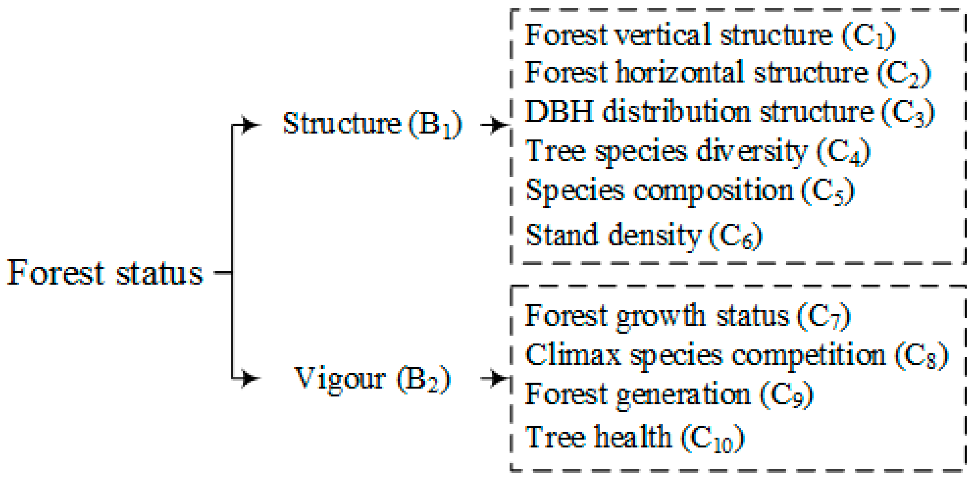
In order to build the evaluation index system of forest state [1], 10 indices were selected, 6 from the forest structural point of view B 1 (vertical structure C 1 , horizontal structure C 2 , DBH distribution structure C 3 , tree species diversity C 4 , species composition C 5 , and stand density C 6 ) and 4 indices regarding forest vigor B 2 (forest growth status C 7 , climax species competition C 8 , forest generation C 9 , and tree health C 10 ) (Figure 2). There was no prior information about the weights Hui et al. [1] placed on the 10 primary attributes. For this reason, the analysis was based on the hypothetical attribute-weighting schemes, that is, each primary attribute was assigned equal weight and was assumed no specific interactions occur between sets of indices.
The forest vertical structure ( C 1 ) is expressed by forest storeys. Referring to the forest vertical stratification standard of the International Union of Forest Research Organizations (IUFRO), the forest storeys can be divided into 3 vertical storeys according to the dominant height. If trees with height ≥2/3 dominant height, they are overstorey trees, if trees with height ≤1/3 dominant height, they are understorey trees, and if trees height are between 1/3 and 2/3, they belong to the middle storey [26]. If the number of trees of each forest storey is greater than or equal to 10%, the forest storey number is 3, meaning it is a multi- storey forest and is assigned a value of 1. If the proportion of tree number in two of the forest storeys is greater than or equal to 10%, the number of forest storeys is 2, meaning it is a multiple storeyed forest and is assigned the value 0.5. If the proportion of trees with only 1 storey is greater than 10%, the number of forest storey is 1, meaning it is a single storey forest, and is assigned a value of 0 [1].
The forest horizontal structure ( C 2 ) is analyzed by uniform angle index (Wi) [27]. Wi describes the degree of regularity in the spatial distribution of four trees that are nearest to a reference tree i, defined as the proportion of the angles α between two adjacent neighbors that are smaller than the standard angle α 0   ( 72 ° ) . The distribution pattern is random distribution if the mean values of W belonging to the confidence interval (0.475, 0.517), otherwise, the pattern is classified as clumped (W > 0.517) or regular (W < 0.475). The random, clumped and regular distribution are assigned the value 1, 0.5 and 0, respectively [1].
W i   =   1 4 j   =   1 n z i j ,     z i j   =   { 1 ,   if   the   angle   α   between   two   adjacent   neighbours is   smaller   than   the   standard   angle   α 0   ( 72 ° ) 0 ,   othersize
The DBH distribution structure ( C 3 ) is commonly used to analyze the population structure and dynamics instead of age structure [28]. The DBH distribution structure with inverted “J” shape reflects the age structure characteristics of uneven-aged forest (selection forest) [24,29], and it is assigned the value 1. When a diameter distribution curve diverts from the regular inversed J shape and presents two or more modals (bimodal, multimodal) then this means that the forest is not an incomplete uneven aged but rather an irregular selection forest or a group selection forest with two or three age classes, and it is assigned 0.5. The unimodal DBH distribution means one storey even aged forest, and it is assigned 0.
The tree species diversity ( C 4 ) is expressed by the mean value of modified species mingling [30]. The calculating formula is
M ¯ =   1 5 N ( M i n i )
M i   =   1 4 j   =   1 n v i j ,     v i j   =   { 1 ,   if   neighbour   j   is   same   species   as   reference   tree   i   0 ,   othersize    
where N is the number of trees in forest; mingling ( M i ) is used to express the segregation of different species in mixed forest, defined as the proportion of the four nearest neighbors that are a different species from the reference tree [31]; n i is tree species number in structural unit in the structure unit in which the ith tree serves as the reference tree. The value of M ¯ is between (0, 1), the bigger the value, the higher the mingling degree is.
The tree species composition ( C 5 ) is calculated according to the relative basal area (RBA) (RBA = BA of species i / B A   of   all   species ) × 100 [32]. If the number of tree species with basal area accounting for more than 10% is greater than or equals to 3, it is the multiple dominant tree species mixed forest and it is assigned a value of 1. If the number is 2, it is the mixed forest and is assigned a value of 0.5. If the number is smaller than 2, it is pure forest and is assigned a value of 0.
The stand density ( C 6 ) is described by the forest crowding degree (K) [33]. K is calculated based on the forest mean crown width of trees (CW), which directly reflects the forest area of photosynthesis and mean tree distance among trees (L), which reflects the possibility of forest maximum spatial utility. The formula is
K   =   L C W   = 10000 / D / C W
where stem density D is the number of stems per hectare (N·ha−1). If the forest crowding K > 1, this indicates that there are gaps in the canopy, and the vertical projection of the canopy is not fully covering the forest land, meaning the trees are not crowded. K = 1 indicates that tree crown contact has just occurred between trees. K < 1 indicates that the trees are too dense. The smaller the K value, the more crowded the forest is. A reasonable interval of K value is between 0.9 and 1.1 and is assigned a value of 1. The stand density is relatively crowded when the K value is between 0.7 and 0. 9, and relatively sparse when the K value is between 1.1 and 1.3 and is assigned the value 0.5 for both cases. In the other cases, the density is either too dense or too sparse, and these situations are assigned a value of 0.
The forest growth status ( C 7 ) is expressed by the stand spatial advantage degree ( S d ) [34], the formula is:
S d = P U i = 0 × G m a x / 2 G m a x G ¯
U i = 1 4 j = 1 n k i j ,     k i j = { 1 ,   if   neighbour   j   is   smaller   than   reference   tree   i   0 ,   othersize    
where DBH dominance ( U i ) [35] is the proportion of the four nearest neighbors of a given reference tree that are smaller than the reference tree i, P U i = 0 is the frequency of trees when these trees are larger than their four nearest neighbors ( U i = 0 ), and G m a x is the potential maximum basal area of forest and is defined as the product of the average basal area of 50% of the larger individuals in the stand times the number of existing trees. G ¯ is the forest basal area. The stand spatial advantage degree ( S d ) is usually bounded between 0 and 1, the bigger, the better.
The climax species competition ( C 8 ) is described by the tree species dominance of climax or target species [4,24], and the formula is:
U s p = R B A g ( 1 U ¯ s p )
R B A g = B A n / B A t × 100 %
where U ¯ s p is the mean dominance of tree species; U s p is bounded between (0, 1), the higher the value, the more dominant the tree species is. B A n is the basal area the nth tree species, B A t is the total basal area of forest, and R B A g is the relative basal area of tree species [32].
The forest regeneration ( C 9 ) is evaluated by the relevant regulations in the “Technical regulations for inventory for forest management planning and design” (GB/T 26424-2010). The measurement of the number of seedlings with height > 50 cm are used. If the seedling density is ≥2500 trees/ha, this indicates that the forest is successfully naturally regenerated, and it is assigned a value of 1. If the seedling density is <500 trees/ha, this indicates that natural regeneration is very poor or irregular, and it is assigned a value of 0. If the seedling density is between 500 and 2500 trees/ha, this indicates that the forest is poorly regenerated, and is assigned a value of 0.5.
The tree health ( C 10 ) refers to the percentage of healthy trees in the forest (no diseases, pests, decayed, hollow, and so forth, and the tree trunk is straight). If the proportion of healthy trees is more than 90%, the assigned value is 1. If the percentage is between (70%, 90%), it is assigned a value of 0.5. If the proportion is less than or equals to 70%, it is assigned a value of 0.

2.3. Methodology

2.3.1. Radar Chart Method

For comparison purposes, the modified radar chart, which is widely used, was selected. The radar chart consists of several equidistant concentric circles and the score of each concentric circle increases gradually from the center of the circle (Figure 3a). N evaluation indices are represented by n radials from the center of the circle; The assigned or calculated values of indices are marked on the index axis and connected with the line segments successively, forming a closed polygon, which is the radar graph of the evaluation object [10,11]. In qualitative analysis, the closer the index value to the center of the circle of the index axis, the smaller the evaluated value is. The evaluation object is visually judged by the overall shape. For quantitative analysis, the area vector in the radar graph should be extracted. The larger the area, the better the evaluation object is, and vice versa [9,11,12]. The calculation formula is as follows:
S i = j = 1 n S i j
S i j = ( I j 1 I j 2 s i n θ ) / 2
where S i is the area of the closed graph in the radar chart of the ith real forest. The higher the value, the better the stand state is. S i j is the area of the closed graph of the jth triangle, which can be obtained by the cosine theorem; I j 1 and I j 2 are the values of the two adjacent indices constituting the jth triangle; θ is the angle of the triangle formed by the two adjacent indices, and it is also the average size of n equilateral angles in the radar graph, that is θ = 2 π / n , where n is the number of indices.

2.3.2. Unit Circle Method

The unit circle is divided into n sector areas, and the radius shared by each two adjacent sector areas is used as the indicator line. The indices are sorted successively according to value and divided into two categories: maximum value 1 and other values. Sorted index values are marked on the radius of the unit circle plot respectively. The maximum value maintains the arc connection, while the other adjacent indices are connected by line segments. The area of the closed graph is a reasonable estimate of the real forest state (Figure 3b). When all index values of forest state are 1, the area of the closed graph is the largest and is equal to the unit circle area, which can be regarded as the expectation value of the optimal forest state. This expectation value is unrelated to the value or the nature of the index, which is the π value rule of the optimal forest state. Therefore, the ratio between the actual stand state and the optimal stand state values is the most appropriate measurement for the real stand state [1], which is expressed by the formula:
S i = { S i 1 + S i 2 π = π m n + i = 1 n m S 2 i π       ( m 2 ) S i 2 π = i = 1 n S 2 i π       ( 0 m < 2 )
S 2 i = ( I 1 I 2 s i n θ ) / 2
where S i is the state value of the ith real forest; S i 1 is the sum of sectorial area in the state diagram of the ith real forest, S i 2 is the sum of the triangle area obtained by the cosine theorem in the ith real forest state graph, n is the number of indices (n ≥ 2), m is the number of indices whose values are equal to 1, I j 1 and I j 2 are adjacent index values of triangle in closed graph, respectively; θ is the angle formed by these two adjacent indices.

2.3.3. New Method Based on Unit Circle

Theoretical Basis

According to the Leaky Bucket Theory and Liebig’s Law of the Minimum [22], a scientific evaluation system should not only accurately describe the functional size of the evaluation object from all aspects but also objectively reflect the inhomogeneity between the indices. In other words, a scientific and reasonable evaluation method involves the unification of the functionality and inhomogeneity of the evaluation system. As mentioned, each index axis represents a normalized index value that is used to calculate the area of the closed graph [10,11]. Therefore, the ratio between the area of the closed graph in the actual stand and the optimal expectation value π in the ideal stand is the most appropriate measurement for the functionality of the real stand state [1]. According to isoperimetric theorem (isoperimetric inequality) [36,37,38], in the closed geometric figure with the same perimeter (P), the area of the circle (A) is the largest. Conversely, in geometric figure with the same area, the perimeter of the circle is the smallest [36,37,38]. This can be expressed as follows:
4 π A P 2
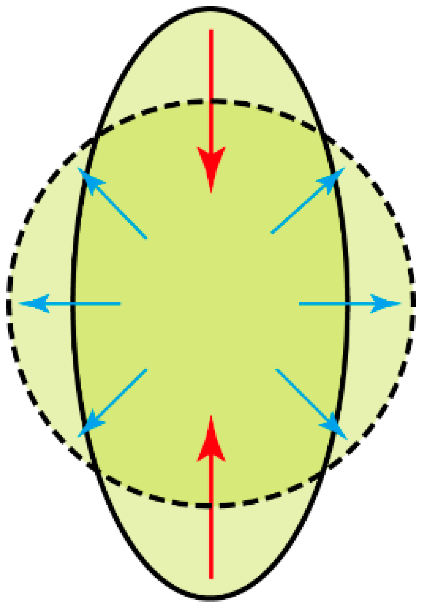
where A stands for area and P is the perimeter of a closed geometric figure. When the closed graph has a certain perimeter, the larger its area, the rounder it tends to be, the more equal the corresponding sequence statistics are, and the more homogeneous the development of the evaluation object from all aspects is [9,11] (Figure 4). Therefore, the arc length of the closed graph in the unit circle can be used to assess the inhomogeneity of evaluation objects. Finally, a comprehensive evaluation model was built based on the geometric mean method of the unique area and arc length to synthetically and simultaneously analyze the functionality and inhomogeneity of the evaluation objects.

Specific steps

In order to eliminate the influence of dimension and dimension units, normalization treatment were carried out using the assignment method according to the biological significance of each index. For example, according to the uniform angle index, the random (0.475 ≤ W ≤ 0.517), clumped (W > 0.517), and regular (W < 0.475) horizontal distribution pattern were assigned the value 1, 0.5 and 0, respectively. In some cases, the evaluation index is not always strictly isotropic. Therefore, it was necessary to transform the negative index ( I i j ) to a positive index ( I i j ) using the reciprocal transformation method, I i j = 1 / I i j . After the above steps, all the evaluation indices were strictly positive and their values were between 0 and 1; the larger the index value, the better the evaluation objective is [1]. As such, the index vector v i = ( v i 1 , v i 2 , , v i n ) of the ith evaluated objective was obtained.
The next step is graph drawing. This involves drawing a unit circle and dividing it into n equal sector areas representing n indicators. The concentric circles are drawn successively with each index value of the real forest as the radius, and the arcs corresponding to the equal sector are retained. The arc and the adjacent two radii form the representative sectors of each index (index sector); the radius shared by two adjacent sectors and the intersection point of their respective arcs are respectively connected by a line segment to form a closed graph including the whole forest (Figure 3c).
Thirdly, the feature vector is extracted. Assume that α i represents the eigenvector of the ith evaluation object; S i and L i represent the area and arc length of the closed graph for the ith evaluation object, respectively, and s i j and l i j represent the area and arc length of the jth indicator sector in the closed graph of the ith evaluation object, respectively. Thus, the eigenvector of the ith evaluation object is α i = ( S i ,   L i ) .
S i = j = 1 n s i j = j = 1 n ( π v i j 2 / n )
L i = j = 1 n l i j = j = 1 n ( 2 π v i j / n )
where v i j is the jth index of the ith evaluation object; n is the number of evaluation indices and is also the number of equilateral sector.
Next, the evaluation vector is constructed. Based on the characteristic vectors S i and L i of the ith evaluation object, β i is the evaluation vector of the ith evaluation object, which is β i = ( β i 1 ,   β i 2 ) (i = 1, 2 …).
β i 1 = S i / S m a x = S i / π
β i 2 = S i / ( π ( L i / 2 π ) 2 ) = 4 π S i / L i 2
When all indices equal to 1, all aspects of the forest state achieve the best condition. In this case, the closed graph is the largest, and is identically equal to the area of the unit circle, S m a x = π . It can be considered the expectation value of the optimal forest state and can be regarded as the π value rule of the optimal state of forest. This is similar to the results of Hui et al. [1], who first proposed the π value rule of the optimal state in natural mixed forest. β i 1 ,   β i 2 ∈(0, 1), where β i 1 reflects the relative area size of the closed figure in the unit circle for the ith estimated forest. The greater the value, the better the forest state is. β i 2 is the ratio between the area of the closed graph in the unit circle of the ith forest state and the area of the circle with the same circumference, reflecting the inhomogeneity degree of all indices regarding forest state. The greater the value, the more balanced the indices of the forest state are.
In the fifth step, evaluation function is construct. The evaluation vector β i is a two-dimensional vector, so the geometric mean method can be used to construct a comprehensive evaluation function F i that simultaneously considers both the functionality and inhomogeneity of the stand state, which is:
F i = f ( β i 1 ,   β i 2 )   =   β i 1 β i 2
where F i is the comprehensive evaluation value of the stand state for the ith real forest. The higher the F i value, the better the overall stand state of the ith forest is.

2.4. Data Analysis

Each index of forest state for the Q. aliena var. acuteserrata broad-leaved mixed forest in the Xiaolong Mountains Forest Region of Gansu Province and the P. koraiensis broad-leaved mixed forest in Jilin Province was calculated separately, and normalization and positive treatment of these indices were carried out [1]. The normalized values of each index were marked in radar graph and unit circle, and the characteristic statistics (area and circumference or arc length) of the closed graph were extracted to quantitatively compare the effectiveness of different methods. Data processing and plot drawing were performed using Excel 2016 and Visio 2013 (Microsoft Corporation, Washington, DC, USA), Origin 2015 (OriginLab Corporation, Washington, DC, USA), and Adobe illustrator CS5 (Adobe, California, CA, USA).

3. Results

3.1. Forest State Characteristics

The characteristics values of different natural forests show that the forest storey of the Q. aliena var. acuteserrata broad-leaved mixed forest (i.e., stands (1) and (2) in Table 2) is 1.9, and its DBH distribution is an inverted J shape, meeting the DBH distribution characteristics of a typical natural uneven-aged mixed forest [24]. The number of regeneration seedlings with height >50 cm reached 8100 trees/ha and 7480 trees/ha, respectively, indicating that the forest is successfully regenerated; but both were relatively crowded. Stand (1) is randomly distributed and highly mixed, with good growth status for the overall stand, obvious competition advantages of the climax tree species and a high proportion of healthy trees. Stand (2) is a mixed forest with multiple dominant tree species and a uniform horizontal distribution pattern; the tree species diversity, growth status, and competitive potential of dominant species are relatively worse; and the proportion of healthy trees is relatively lower.
The P. koraiensis broad-leaved mixed forest (i.e., stands (3) and (4) in Table 2) are all randomly distributed, and its DBH distribution is an inverted J shape. The proportion of healthy trees is over 90%; both are crowded and regenerated poorly. Stand (3) is a multi-storey mixed forest, with relatively lower mixing degree, and the competitive potential of the climax tree species is not obvious. Stand (4) is a mixed forest with multiple dominant tree species, and tree species diversity and competition potential of the climax tree species are relatively higher but it has only 2 forest storeys.

3.2. Radar Plot Method

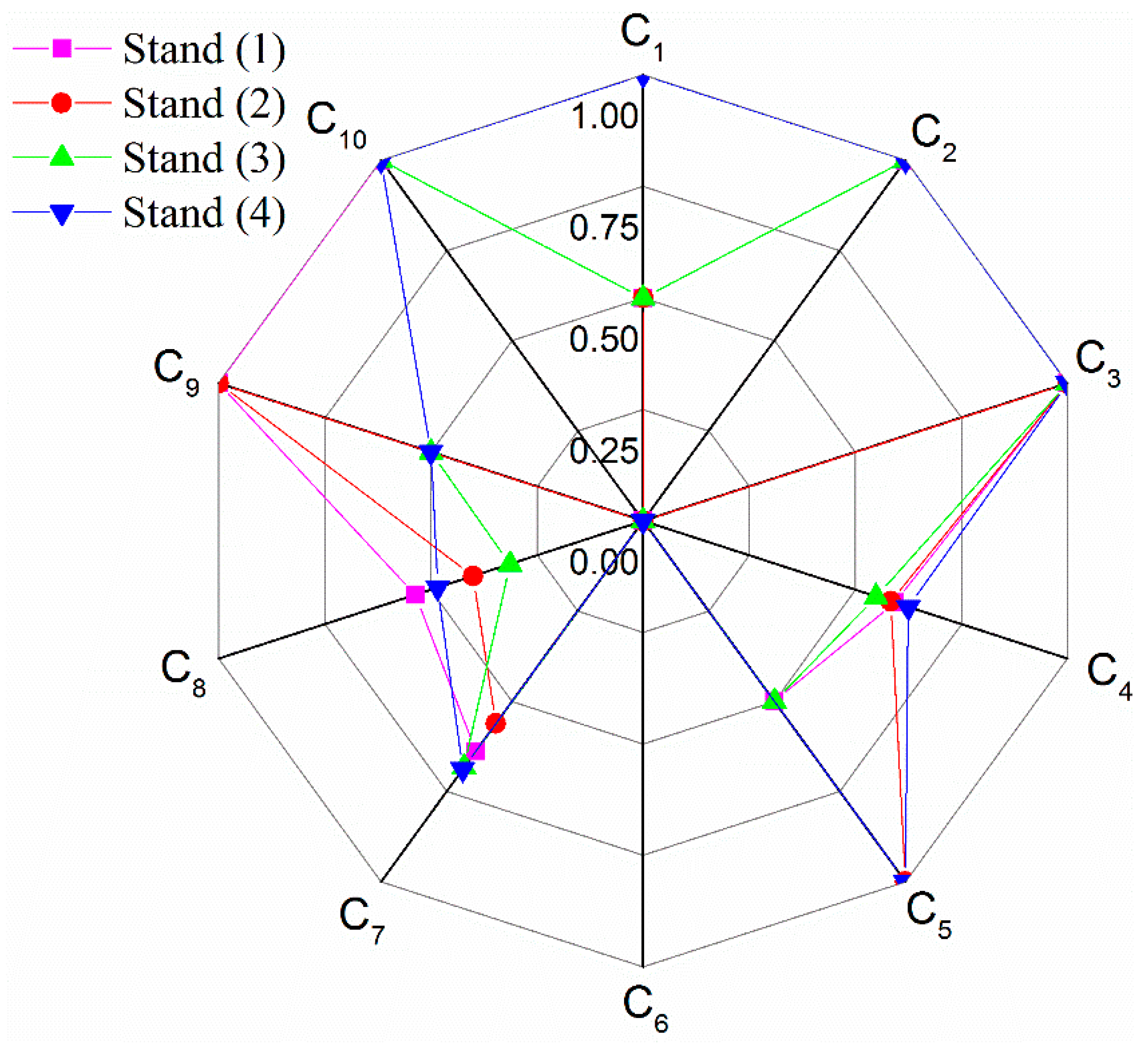
As illustrated in Figure 5, the radar diagram visualizes the relative values of 10 aspects of forest state. Specifically, stand (1) is a well-regenerated, uneven aged forest and is randomly distributed as a whole; most of the individuals are in good health but forest density is too dense. Stand (2) is a well-regenerated, uneven aged forest with multiple dominant tree species. However, it has a uniform horizontal distribution pattern with too dense individuals and 13.9% unhealthy trees. Compared with stand (4), stand (3) only has two forest storeys and two dominant tree species with basal area more than 10% but its regeneration is better than stand (4). Notably, the forest density of Q. aliena var. acuteserrata broad-leaved mixed forest and the P. koraiensis broad-leaved mixed forest are too dense ( C 6 ). Density is the key factor restricting the forest state, so measures must be adopted to solve the problems. Overall, the radar map method can be used to compare the relative merits of different stands from all aspects and shows strong performance but single index considerably influence the area of two adjacent triangles and the whole closed figure area. For example, the forest density ( C 6 ) equals 0 . As a result, C 5 , C 6 and C 6 , C 7 cannot form effective triangles with the center of the circle, so the area of its two adjacent triangles are both equal 0, directly affecting the total area of the closed graph in the radar plot (Figure 5).

3.3. Unit Circle Method

As described in Figure 6, the relative states of the stands are clear and visualized based on the unit circle method. Among them, stand (1) obtained the optimal value of 1 in terms of horizontal structure, age structure, forest regeneration and tree health. This was followed by the growth status and species diversity, with values of 0.584 and 0.562, respectively. The value of forest density is 0. Stand (2) has an optimal DBH distribution structure, tree species composition and forest regeneration, followed by higher tree species diversity and better growth status but the forest density and health are deficiency. Stand (3) received the best value in terms of horizontal structure, age structure and forest health, followed by the growth status and tree species diversity, which have higher value but the forest density is too dense. Stand (4) is optimal in five aspects and has a good growth state and complex tree species composition. Therefore, the unit circle method has a good performance for graphing the states of single stand, and the relative values of each index are clear; the feature statistics (area and perimeter) of the closed graph are relatively unique after each index is sorted. Each forest needs to be graphed individually and the indices are not in the same order after ranking, so visual contrasts between different forests are not obvious.
The value of a single index directly affects the value of statistic feature (i.e., area and perimeter). For example, when forest density ( C 6 ) is equal to 0, the characteristic values of the two adjacent areas are also 0, therefore, effective measurement values for the overall of forest state cannot be determined. In other words, though the values of the forest density ( C 6 ) and its two adjacent areas are 0, the number of the index ( C 6 ) and adjacent areas, whose value is equal to 0, are 1 and 2, respectively, they are not equal in quantity, indicating that a single index has a greater impact on the overall evaluation results.

3.4. New Method Based on the Unit Circle

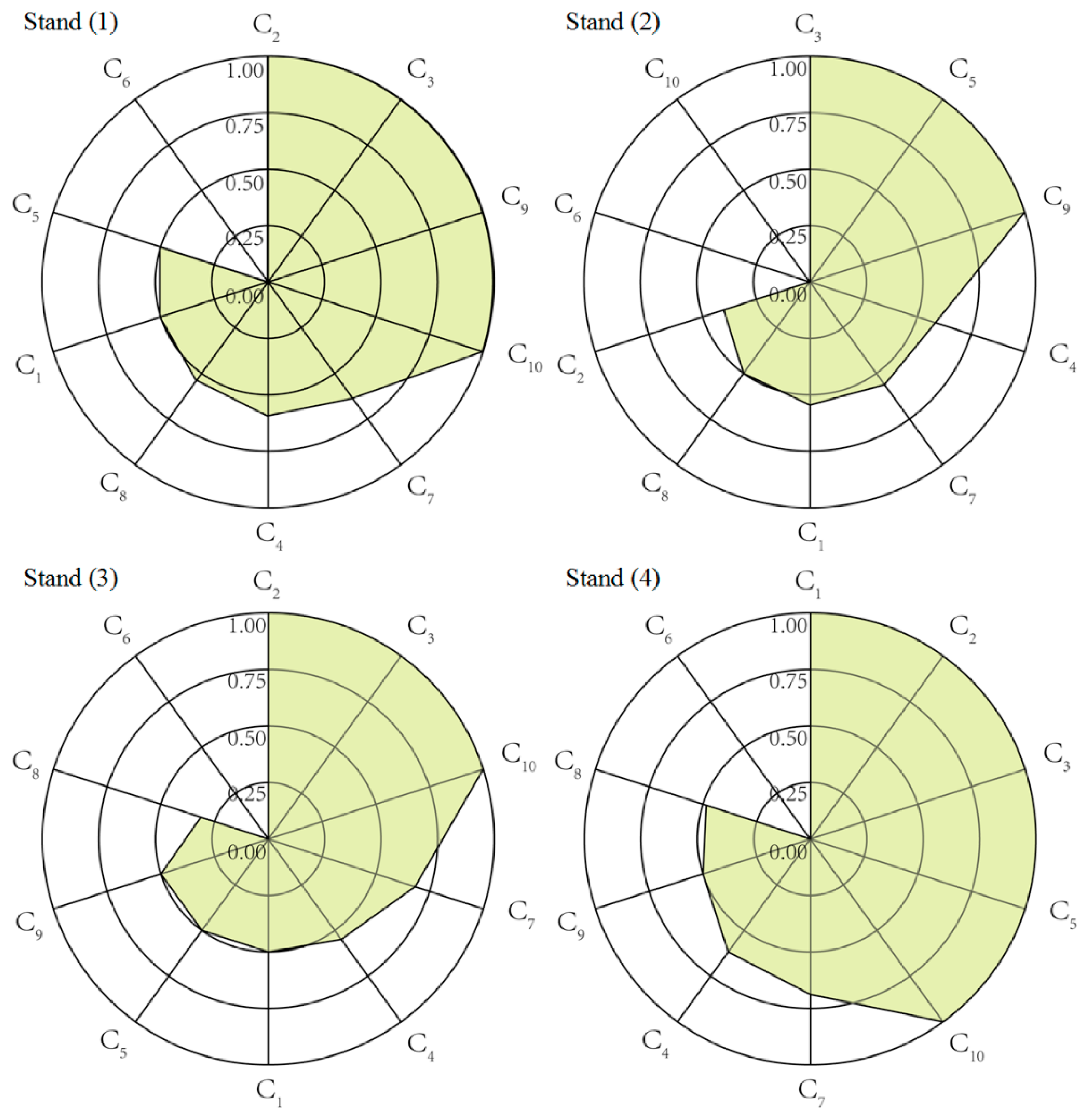
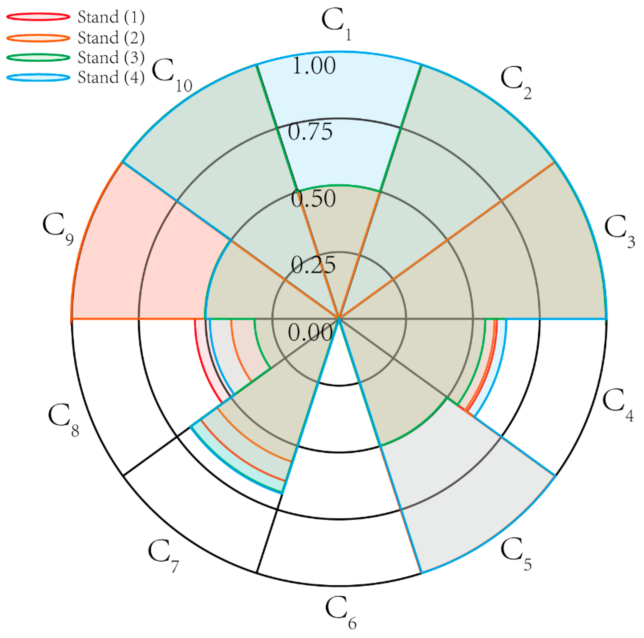
According to the new method based on unit circle (Figure 7), in terms of forest structure, all four natural forests demonstrate DBH distribution characteristics typical of uneven-aged forests, with stand density being too dense. The horizontal pattern of stand (2) is uniformly distributed, obviously limiting the forest healthy state. The remaining structural states of the four stands all appear adequate. In terms of forest vitality, the proportion of healthy trees in stand (2) is small, and the remaining stands have mostly healthy trees. The Q. aliena var. acuteserrata broad-leaved mixed forest successfully naturally regenerated, and the P. koraiensis broad-leaved mixed forest poorly regenerated. The difference between the two types of forests in terms of growth status and climax species competition is particularly prominent. As a consequence, with the newly proposed unit circle method, a single index is represented by an independent sector area whose area depends on the value of the index itself and reflects the contribution of the index to the whole. The characteristic value of the formed closed graph (i.e., area and arc length) and evaluation results are unique. The graph comprehensively captures the evaluation index, and the evaluation result does not depend on the order and value of the indices, which facilitates a comparative study of different evaluation objects and satisfies the graphics presentation requirements of multivariate comprehensive evaluations.

3.5. Comparison of Evaluation Results Based on Different Methods

According to the comprehensive evaluation value based on the radar graph method and unit circle methods (Table 3), the forest state ranking is consistent with previous research results [1]. It can be seen from the area quantity of the new method based on the modified unit circle, that the functionality evaluation results of the four forests are (1) 0.555, (2) 0.407, (3) 0.462 and (4) 0.635, which is consistent with the research results of the first two methods. The inhomogeneity evaluation results are 1.211, 1.597, 1.263 and 1.192, respectively. Stand (2) is relatively inhomogeneous in all aspects, followed by stand (3). Stand (4) had the biggest difference in terms of indices inhomogeneity. Based on the evaluation results of these two factors, we determined that the comprehensive evaluation values of the four stands were 0.820, 0.806, 0.764 and 0.870, respectively. Thus, the advantages of stand (4) and stand (1) are obvious in many aspects but their stand density is too dense, restricting the comprehensive and sustainable development of forest. The forest densities of stands (4) and (1) should therefore be adjusted first via forest management practices. Stands (2) and (3) are relatively inhomogeneous in all aspects but their advantages are not obvious. Therefore, multiple management measures should be implemented simultaneously to improve the production of the whole forest in all aspects. Notably, the synthetic sorting results of the proposed method are inconsistent with those of the radar chart method or unit circle method. Although each index in stand (3) is relatively larger, the inhomogeneity index of the stand is only 1.263, much smaller than that of stand (2) ( β i 2 = 1.597). This produces the combined evaluation results of 0.806 and 0.764, suggesting that stand (2) is in a better state than stand (3). These results indicate that the new method based on the unit circle more accurately reflects the differences among evaluated objects and effectively avoids possible evaluation deviations and misjudgments.

4. Discussion

4.1. Compared with Statistics-Based Methods

A comprehensive evaluation is key for comparative and decision-making analyses. There are many statistics-based methods, such as comprehensive index method [39], analytic hierarchy process [40], fuzzy mathematics method [41,42], multiple criteria decision making approaches [43,44], support vector machine [39,45], random forest [46], artificial neural networks [47], and Topsis method [42]. These methods are of great importance to qualitatively or quantitatively evaluate forest fire, forest sustainability, ecosystem management alternatives, and more. [39,40,41,42,43,44,45,46,47]. However, some problems remain, such as the selection of the evaluation factors not being sufficiently comprehensive and objective, and unreasonable comprehensive evaluation methods with subjective factors and complex weight calculations lead to the evaluation results lacking comparability [39]. One of the biggest problems is that conventional data presentation method lack intuitive and decision-making visualization. Assessment information in the aforementioned studies was expressed by text or tables featuring a single form and low visualization [6]. With the complexity and uncertainty of forestry resources data (i.e., multidimensional, dynamic, multi-source, multi-scale, and spatial variable data), these two factors lead to the phenomenon of data rich but information poor in forestry research [7]. Therefore, the graphical display of the evaluation information has become urgently required. The radar map, unit circle, and improved unit circle methods are intuitive, greatly improving our understanding and acceptability of the comprehensive evaluation information [7,40].

4.2. Compared with Geometry-Based Methods

Compared with text or tables, graphical displays are particularly suitable for concisely illustrating data patterns, relationships and trends [10,48]. Simple graphs, such as bar chart, trend chart, and pie chart, usually compare or present limited data. Complex multivariate data can be visualized by glyphs, Andrews’ curves, Chernoff faces, and other such methods. [49]. Among them, the spie chart [10,50], target plot [10,51], radar plot [10,16,48], and unit circle [1,5] intuitively graph multivariate data and are therefore useful for providing understandable summaries of evaluation information.
Spie charts, consisting of two superimposed pie charts [10], are unique in using both angles and radii (and as a result, area) to convey data. The spie chart was designed specifically for comparing one partition to another [50], summarizing the overall performance of an evaluation object with a global score [10]. A possible criticism of spie charts is that they are particularly dependent on the relative importance attributed to the investigated categories [10]. It may be especially hard to estimate the relative sizes of slices that have different angles, radii, and orientations [50] due to the fact that estimating areas is much less precise than estimating lengths [52].
Target plots simultaneously display multiple performance indicators at the level of single evaluation object [51]. Indicators of good performance are closer to the center, and indicators of poor performance are closer to the target periphery [10]. The score of each dimension permits immediate interpretation; however, the target plots fail to distinguish categories (the “dots”) with values that are approximate or superimposed [51].
As a form of radial graphing, radar plots are composed of radii that are projected from the graph center, and the length of an individual radius corresponds to the measured value (Figure 5). These values are usually connected to form an enclosed shape [10] and the sum of the formed triangle area is taken as the measurement basis [13,14,17,39]. The radar plot is useful for the presentation of multivariate data, especially in situations in which there are many independent variables, possibly with different measurement scales. However, interpretation of the results strongly depends on the ordering of the indices being displayed [10,48], so the graphical features extracted by areas and perimeters are not unique [12], which can lead to misunderstanding and misjudgment.
In contrast, the unit circle method first sorts each index according to its value. The arc-shaped connection is adopted among the maximum values, and the remaining indices are connected by line segments. Secondly, the sector areas and triangle areas are summed as the total measurement values. The total area of the closed graph is relatively unique, and the evaluation results objectively reflect the forest state to some extent. Unfortunately, the ranking order of evaluation indices in different forest types or different periods is not completely consistent (Figure 6), seriously limiting intuitive comparison usefulness under different space-time conditions. The main difference between the unit circle and radar map methods is that the expected value of the optimal stand state is independent of forest types and index number or the description of the indices. At This point, the expected value is equal to the area of the unit circle (π). Each index obtains the maximum value of 1 [1]. Both the radar plots and unit circles emphasize the combined effect between two adjacent indices while ignoring the independence of each index and its contribution to the overall function of stand. As a result, a missing or small value of a single index significantly influence the total result.
Compared with the visual graphics mentioned above, our proposed method based on the unit circle has many advantages. Each sector region independently represents a single evaluation index, reflecting the contribution of each index to the overall evaluation result and avoiding the aggregated or superimposed dots of target plots [51]. The area and arc length of each sector region are unique, overcoming the possible non-uniqueness of statistic features found in the radar plots [10,17,48,53]. The four forests share the same index sequence in the modified unit circle, facilitating horizontal and vertical comparison among different evaluation objects. The incomplete consistency of index order that occurred in the unit circle method [1] was avoided. Every sector region has an equal central angle, meaning that each index has the same relative importance weight. This contributes to estimating the relative sizes of slices and summarizing the overall performance of an objective with a global score, which is superior to the spie chart methods [10,50]. The proposed method evaluates the functionality and inhomogeneity of the evaluation object simultaneously, whereas most previous studies only focused on forest functionality [1,13,14,17,39]. Furthermore, our method meets the visual presentation requirements of multilevel and overall evaluation results.

4.3. Implications for Decision-Making Regarding Forest Management

The newly proposed comprehensive evaluation method is a powerful tool for the diagnosis of forest state problems and the decision-making of forest management. It is more efficient than the unit circle method used in previous studies [1,5]. Concentric circles in the unit circle with values of 1.00, 0.50, and 0.25 represent the baseline of the best, average and worse stand state, respectively. A value of any index less than 0.5 is considered as an unqualified index [5]. Therefore, according to the poor indices of different forest states (mostly caused by management issues), management measures should be prioritized to solve the main forest state problem [5]. For example, stand (1) is relatively healthy and stable in most aspects but forest density is too dense (K = 0.633), being a restrictive factor on the sustainable development of the stand. It is thus necessary to carry out cutting or pruning [54]. The inhomogeneity value of stand (2) is higher ( β i 2 = 1.597) than those of the other stands, suggesting that stand (2) is undergoing unbalanced development in some aspects of forest states. Specifically, the trees in stand (2) are uniformly distributed and too dense, featuring weak competitive potential of climax species and slightly fewer healthy trees. Management measures should thus be implemented jointly to comprehensively improve the quality of the stand. These measures should simultaneously include single-tree selection cutting [55] of unhealthy individuals, the adjustment of the competitive environment of the climax tree species, and the regulation of horizontal tree distribution pattern and forest density, simultaneously.
The majority of the forest state characteristics of stand (3) were similar to those of stand (4) but they are both too dense and exhibit the weak competition potential of climax species, so priority should be given to forest density regulation and the adjustment of the competitive microenvironment of climax species. Hui et al. [5] explored natural forest management measure priorities based on the unit circles of forest states and proposed 120 different natural forest management actions based on stand state combinations. However, this method proposed management strategies targeted only at functionality. The new proposed method clearly identifies the key factors affecting the forest states according to the values of each index and the inhomogeneity among different indices. These results have profound implications for management strategies, which are implemented following the aim of comprehensively improving stand quality and effectively promoting the sustainable development of the forest.

5. Conclusions

A novel forest state comprehensive evaluation method was proposed based on the isoperimetric theorem (isoperimetric inequality), simultaneously highlighting the functionality of each evaluation index and the inhomogeneity among different evaluation indices. The modified unit circle visualizes the evaluation information. The areas and the arc lengths of each sector region are unique, independently reflecting the contribution of each index to the overall result. Different evaluation objectives share the same index sequence and equal central angles, facilitating comparative analysis and summarizing the overall performance. This method is a powerful tool for the diagnosis of forest state problems and for the decisions-making of forest management.

Author Contributions

Data curation, Y.H. and Z.Z.; Investigation, Y.H. and Z.Z.; Methodology, G.Z. (Ganggang Zhang) and G.H.; Software, G.Z. (Gongqiao Zhang); Visualization, G.Z. (Gongqiao Zhang); Writing—original draft, G.Z. (Ganggang Zhang); Writing—review & editing, G.Z. (Ganggang Zhang) and G.H.

Funding

This research was funded by the National Key Research and Development Program of China (2016YFD0600203).

Acknowledgments

We thank two anonymous reviewers for helpful comments on earlier versions of this manuscript.

Conflicts of Interest

The authors have declared that no competing interests exist.

References

  1. Hui, G.Y.; Zhang, G.Q.; Zhao, Z.H.; Hu, Y.B.; Liu, W.Z.; Zhang, S.Z.; Bai, C. A new rule of π value of natural mixed forest optimal stand state. Sci. Silvae Sin. 2016, 52, 1–8. [Google Scholar] [CrossRef]
  2. Wu, J.Y.; Shi, B.S. The affecting analysis of appraisal model to appraisal reliability. Syst. Eng. Theory Pract. 1993, 13, 11–15. [Google Scholar] [CrossRef]
  3. Zhang, G.Q.; Hui, G.Y. A new design of field trial for forest management based on stand characteristics. For. Res. 2015, 28, 145–151. [Google Scholar] [CrossRef]
  4. Zhao, Z.H.; Hui, G.Y. Forest naturalness evaluation method based on stand state characters: A case study of Gansu Xiaolongshan Forests. Sci. Silvae Sin. 2011, 47, 9–16. [Google Scholar] [CrossRef]
  5. Hui, G.Y.; Zhao, Z.H.; Zhang, G.Q. Priority of management measures for natural forests based on the stand state. J. Beijing For. Univ. 2016, 38, 1–10. [Google Scholar] [CrossRef]
  6. Lu, D.M.; Wang, Z.M.; Fu, H.L. Design of forestry resources statistical data visualization system based on WebGIS. World For. Res. 2017, 30, 46–51. [Google Scholar] [CrossRef]
  7. Wang, Z.G.; Zhuang, D.F.; Qiu, D.S.; Ming, T. Application analysis of data mining and visualization in forestry. Geo-Inf. Sci. 2007, 9, 19–22. [Google Scholar] [CrossRef]
  8. Qi, Y.R. The Method of Determining Index Weight and Its Application Research. Master’s Thesis, Northeastern University, Shenyang, China, June 2010. [Google Scholar] [CrossRef]
  9. Du, W.; Wang, C.Q.; Li, B.; Li, B.; Zhang, Z.J.; Lei, B. Application of optimized radar-graph method on comprehensive evaluation of appearance quality of upper leaves of flue-cured tobacco. Chin. Tob. Sci. 2015, 36, 24–29. [Google Scholar] [CrossRef]
  10. Stafoggia, M.; Lallo, A.; Fusco, D.; Barone, A.P.; D’Ovidio, M.; Sorge, C.; Perucci, C.A. Spie charts, target plots, and radar plots for displaying comparative outcomes of health care. J. Clin. Epidemiol. 2011, 64, 770–778. [Google Scholar] [CrossRef]
  11. Zheng, H.L.; Liu, C.; Zhai, D.N. Comprehensive evaluating method based on radar-graph. J. Nanjing Univ. Posts Telecommun. 2001, 21, 75–79. [Google Scholar] [CrossRef]
  12. Wang, Y.Y. The existing problems and improvement measures of the quantitative comprehensive evaluation method based on radar map. Stat. Educ. 2007, 1, 18–20. [Google Scholar]
  13. Ying, M.F. Study on Multi-Functional Evaluation of Plantation Forest in Da Biangou Forest Center. Ph.D. Thesis, Beijing Forestry University, Beijing, China, June 2011. [Google Scholar]
  14. Sun, X.Q. Study on Multi-Functional Evaluation of Forest in Culai Forest Farm. Master’s Thesis, Shandong Agricultural University, Tai’an, China, December 2015. [Google Scholar]
  15. Li, C.B.; Qi, J.G.; Wang, S.B.; Yang, L.S.; Zou, S.B.; Zhu, G.F.; Yang, W.J. Spatiotemporal characteristics of alpine snow and ice melt under a changing regional climate: A case study in Northwest China. Quat. Int. 2015, 358, 126–136. [Google Scholar] [CrossRef]
  16. Frank, S.; Fürst, C.; Pietzsch, F. Cross-sectoral resource management: How forest management alternatives affect the provision of biomass and other ecosystem services. Forests 2015, 6, 533–560. [Google Scholar] [CrossRef]
  17. Thomas, P.A.; Mukassabi, T.A. Biological Flora of the British Isles: Ruscus Aculeatus. J. Ecol. 2014, 102, 1083–1100. [Google Scholar] [CrossRef]
  18. Thivierge, M.N.; Parent, D.; Bélanger, V.; Angers, D.A.; Allard, G.; Pellerin, D.; Vanasse, A. Environmental sustainability indicators for cash-crop farms in Quebec, Canada: A participatory approach. Ecol. Indic. 2014, 45, 677–686. [Google Scholar] [CrossRef]
  19. Mendoza, G.A.; Dalton, W.J. Multi-stakeholder assessment of forest sustainability: Multi-criteria analysis and the case of the Ontario forest assessment system. For. Chron. 2005, 81, 222–228. [Google Scholar] [CrossRef] [Green Version]
  20. Vallsdonderis, P.; Vallésplanells, M.; Galiana, F. Short communication: AHP for indicators of sustainable forestry under Mediterranean conditions. For. Syst. 2017, 26, 1–5. [Google Scholar] [CrossRef]
  21. Ochoa-Gaona, S.; Kampichler, C.; de Jong, B.H.J.; Hemández, S.; Geissen, V.; Huerta, E. A multi-criterion index for the evaluation of local tropical forest conditions in Mexico. For. Ecol. Manag. 2010, 260, 618–627. [Google Scholar] [CrossRef]
  22. Hooker, H.D. Liebig’s Law of the Minimum in Relation to General Biological Problems. Science 1917, 46, 197–204. [Google Scholar] [CrossRef] [PubMed]
  23. Yang, W.C.; Xu, K.; Lian, J.J.; Ma, C.; Bin, L.L. Integrated flood vulnerability assessment approach based on TOPSIS and Shannon entropy methods. Ecol. Indic. 2018, 89, 269–280. [Google Scholar] [CrossRef]
  24. Hui, G.Y.; Zhao, Z.H.; Hu, Y.B. A Guide to Structured-Based Forest Management; China Forestry Publishing House: Beijing, China, 2010; ISBN 978-7-5038-5765-2. [Google Scholar]
  25. Pommerening, A.; Stoyan, D. Edge-correction needs in estimating indices of spatial forest structure. Can. J. For. Res. 2006, 36, 1723–1739. [Google Scholar] [CrossRef]
  26. Kramer, H. Waldwachstumslehre; Paul Parey: Hamburg/Berlin, Germany, 1988. [Google Scholar]
  27. Hui, G.Y.; Gadow, K.V.; Albert, M. The neighbourhood pattern—A new structure parameter for describing distribution of forest tree position. Sci. Silvae Sin. 1999, 35, 37–42. [Google Scholar] [CrossRef]
  28. Song, Y.C. Vegetation Ecology; East China Normal University Press: Shanghai, China, 2001; ISBN 978-7-0404-6159-6. [Google Scholar]
  29. Meyer, H.A. Structure, growth and drain in balanced uneven-aged forests. J. For. 1952, 50, 85–92. [Google Scholar]
  30. Hui, G.Y.; Hu, Y.B.; Zhao, Z.H. Evaluating tree species segregation based on neighborhood spatial relationships. J. Beijing For. Univ. 2008, 30, 131–134. [Google Scholar] [CrossRef]
  31. Hui, G.Y.; Hu, Y.B. Measuring species spatial isolation in mixed forests. For. Res. 2001, 14, 23–27. [Google Scholar] [CrossRef]
  32. Rybicki, N.B.; Noe, G.B.; Hupp, C.; Robinson, M.E. Vegetation composition, nutrient, and sediment dynamics along a floodplain landscape. River Syst. 2015, 21, 109–123. [Google Scholar] [CrossRef]
  33. Hui, G.Y.; Zhang, L.J.; Hu, Y.B.; Wang, H.X.; Zhang, G.Q. Stand crowding degree and its application. J. Beijing For. Univ. 2016, 38, 1–6. [Google Scholar] [CrossRef]
  34. Zhao, Z.H.; Hui, G.Y.; Hu, Y.B.; Li, Y.F.; Wang, H.X. Method and application of stand spatial advantage degree based on the neighborhood comparison. J. Beijing For. Univ. 2014, 36, 78–82. [Google Scholar] [CrossRef]
  35. Hui, G.Y.; Gadow, K.V.; Albert, M. A new parameter for stand spatial structure—neighbourhood comparison. For. Res. 1999, 12, 1–6. [Google Scholar] [CrossRef]
  36. Osserman, R. The isoperimetric inequality. Bull. Am. Math. Soc. 1978, 84, 1182–1238. [Google Scholar] [CrossRef]
  37. Zhang, J.H. The history of the proof on the isoperimetric theorem. J. Guangxi Univ. Natl (Nat. Sci. Ed.) 1995, 1, 111–116. [Google Scholar] [CrossRef]
  38. Kesavan, S. The Isoperimetric inequality. Resonance 2002, 7, 8–18. [Google Scholar] [CrossRef]
  39. Jiang, X.; Lu, W.X.; Zhao, H.Q.; Yang, Q.C.; Chen, M. Quantitative evaluation of mining geo-environmental quality in Northeast China: Comprehensive index method and support vector machine models. Environ. Earth Sci. 2015, 73, 7945–7955. [Google Scholar] [CrossRef]
  40. Marian, D.; Palaghianu, C.; Onciul, M.M. Benefit, cost and risk analysis on extending the forest roads network: A case study in Crasna Valley (Romania). Ann. For. Res. 2015, 58, 333–345. [Google Scholar] [CrossRef]
  41. Shi, Q.; Lu, Z.H.; Liu, Z.M.; Miao, Y.; Meng, J. Evaluation model of the grey fuzzy on eco-environment vulnerability. J. For. Res. 2007, 18, 187–192. [Google Scholar] [CrossRef]
  42. Xu, Z.S.; Zhang, X.L. Hesitant fuzzy multi-attribute decision making based on TOPSIS with incomplete weight information. Knowl.-Based Syst. 2013, 52, 53–64. [Google Scholar] [CrossRef]
  43. Mendoza, G.A.; Prabhu, R. Multiple criteria decision making approaches to assessing forest sustainability using criteria and indicators: A case study. For. Ecol. Manag. 2000, 131, 107–126. [Google Scholar] [CrossRef]
  44. Prato, T. Multiple-attribute evaluation of ecosystem management for the Missouri River system. Ecol. Econ. 2003, 45, 297–309. [Google Scholar] [CrossRef]
  45. Zhao, J.H.; Zhang, Z.; Han, S.Z.; Qu, C.Z.; Yuan, Z.Y.; Zhang, D.Y. SVM based forest fire detection using static and dynamic features. Comput. Sci. Inf. Syst. 2011, 8, 821–841. [Google Scholar] [CrossRef]
  46. Leuenberger, M.; Kanevski, M.; Vega, O.C.D. Forest fires in a random forest. In Proceedings of the European Geosciences Union General Assembly, Vienna, Austria, 7–12 April 2013; Volume 15, p. 3238. [Google Scholar]
  47. Safi, Y.; Bouroumi, A. A neural network approach for predicting forest fires. In Proceedings of the 2011 International Conference on Multimedia Computing & Systems, Ouarzazate, Morocco, 7–9 April 2011; IEEE: Ouarzazate, Morocco, 2011. [Google Scholar] [CrossRef]
  48. Saary, M.J. Radar plots: A useful way for presenting multivariate health care data. J. Clin. Epidemiol. 2008, 61, 311–317. [Google Scholar] [CrossRef]
  49. Toit, S.H.C.D.; Steyn, A.G.W.; Stumpf, R.H. Graphical exploratory data analysis. J. Am. Stat. Assoc. 1986, 31, 116–117. [Google Scholar] [CrossRef]
  50. Feitelson, D.G. Data on the distribution of cancer incidence and death across age and sex groups revealed using multi-level spie charts. J. Clin. Epidemiol. 2016, 72, 90–97. [Google Scholar] [CrossRef]
  51. Nuti, S.; Bonini, A.; Murante, A.M.; Vainieri, M. Performance assessment in the maternity pathway in Tuscany region. Health Serv. Manag. Res. 2009, 22, 115–121. [Google Scholar] [CrossRef] [PubMed] [Green Version]
  52. Cleveland, W.S.; McGill, R. Graphical perception: Theory, experimentation, and application to the development of graphical methods. J. Am. Stat. Assoc. 1984, 79, 531–554. [Google Scholar] [CrossRef]
  53. Dan, R.; Woodhouse, P.; Young, T.; Burton, M. Constructing a farm level indicator of sustainable agricultural practice. Ecol. Econ. 2001, 39, 463–478. [Google Scholar] [CrossRef]
  54. Bauhus, J.; Pyttel, P. Managed forests. In Routledge Handbook of Forest Ecology; Peh, K.S.H., Corlett, R.T., Bergeron, Y., Eds.; Routledge: Oxon, UK, 2015; pp. 75–90. ISBN 978-0415-73545-2. [Google Scholar]
  55. Nyland, R.D. Selection system in northern hardwoods. J. For. 1998, 96, 18–21. [Google Scholar] [CrossRef]
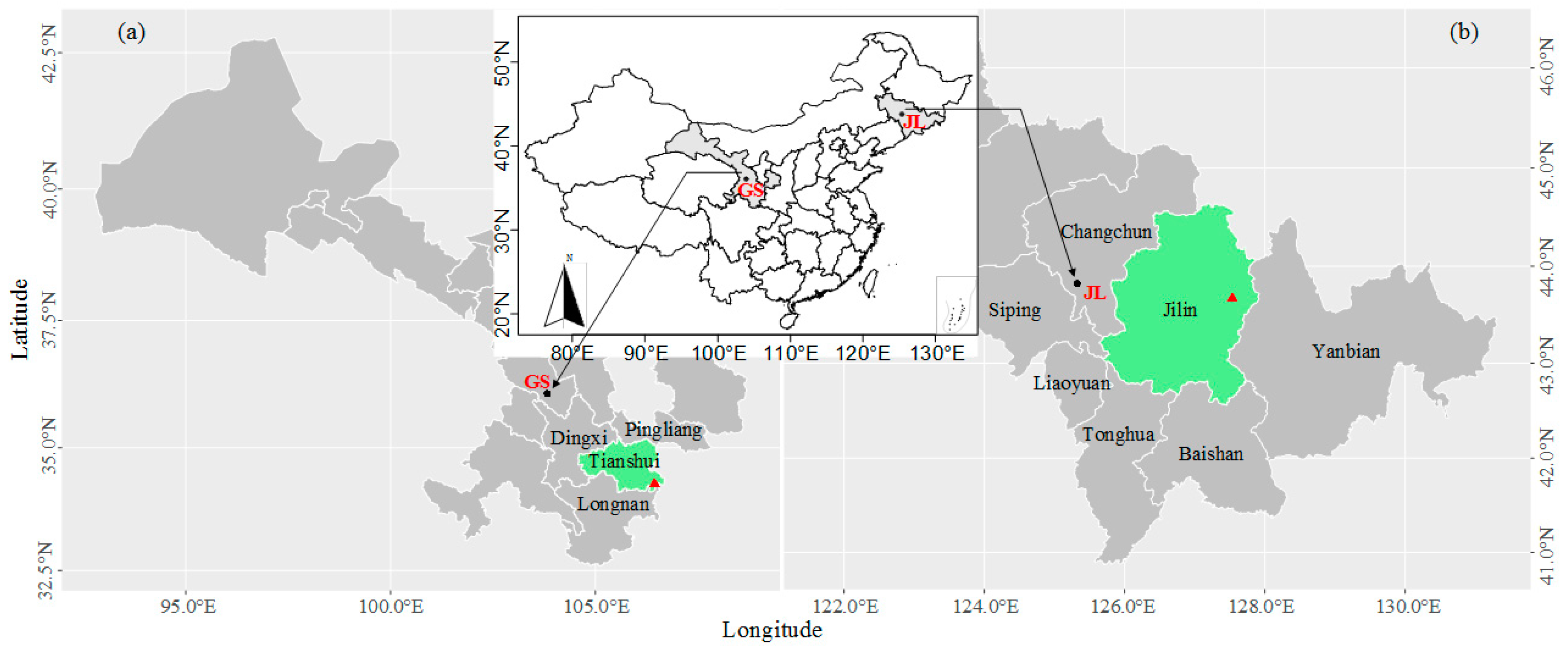
Figure 1. The plot (red triangles) of (a) Quercus aliena BL. var. acuteserrata Maxim. ex Wenz. mixed forest is located in Southeast Tianshui City in Gansu Province (GS), and that of (b) Pinus koraiensis Sieb. et Zucc. broad-leaved mixed forest is located in Eastern Jilin City in Jilin Province (JL), China.
Forests 10 00005 g001
Figure 2. The evaluation index system of forest state.
Forests 10 00005 g002
Figure 3. Radar plot (a), unit circle (b) and modified unit circle (c). C 1 C 10 are ten evaluation indices of stand state respectively.
Forests 10 00005 g003
Figure 4. A long, narrow graph can be flattened to become rounder, making the area larger and the circumference unchanged.
Forests 10 00005 g004
Figure 5. Radar plot of Q. aliena var. acuteserrata broad-leaved mixed forest (stands (1) and (2)) and P. koraiensis broad-leaved mixed forest (stands (3) and (4)).
Forests 10 00005 g005
Figure 6. Unit circle of Q. aliena var. acuteserrata broad-leaved mixed forest (stands (1) and (2)) and P. koraiensis broad-leaved mixed forest (stands (3) and (4)).
Forests 10 00005 g006
Figure 7. New unit circle of Q. aliena var. acuteserrata broad-leaved mixed forest (stands (1) and (2)) and P. koraiensis broad-leaved mixed forest (stands (3) and (4)).
Forests 10 00005 g007
Table 1. Overview of survey sample plot details.
StandForest TypePlot Size (m2)Species No.Slope Gradient (°)Slope AspectAltitude (m)Basal Area (m2·ha−1)Mean DBH (cm)Density (N·ha−1)
(1)Q. aliena var. acuteserrata mixed forest70 × 703312NW172027.919.5933
(2)70 × 703512NW170025.319.6842
(3)P. koraiensis broad-leaved mixed forest100 × 1002017NW66031.318.11186
(4)100 × 100228NW60031.922.1800
DBH is diameter at breast height.
Table 2. State characteristics of different natural forests (original value/normalized value).
Stand Structure   B 1 Vigor   B 2
Vertical   Structure   C 1 Horizontal   Structure   C 2 DBH   Distribution   Structure   C 3 Tree   Species   Diversity   C 4 Species   Composition   C 5 Density   C 6 Growth   Status   C 7 Climax   Species   Competition   C 8 Regeneration   C 9 Tree   Health   C 10
(1)1.9/0.50.492/1Inverted J shape/10.5932/0.50.633/00.6380.5378100/196.5%/1
(2)1.9/0.50.533/0Inverted J shape/10.5843/10.554/00.5620.4017480/187.1%/0
(3)2.2/0.50.499/1Inverted J shape/10.5492/0.50.660/00.6830.3142300/0.590.9%/1
(4)2.5/10.491/1Inverted J shape/10.6253/10.643/00.6880.484720/0.592.9%/1
10 evaluation indices ( C 1 C 10 ) were selected from the forest structure B 1 and forest vigor B 2 .
Table 3. The comprehensive evaluation value of different forests.
StandRadar PlotUnit CircleNew Method Based on Unit Circle
S i Rank S i Rank S i L i β i 1 β i 2 F i Rank
(1)1.40221.61421.7434.2520.5551.2110.8202
(2)0.52741.18041.2783.1710.4071.5970.8063
(3)1.08631.32631.4503.7990.4621.2630.7644
(4)1.56511.86011.9944.5850.6351.1920.8701
In the ith evaluated forest, S i and L i are the area and arc length of the closed graph; β i 1 , β i 2 are the functionality and inhomogeneity evaluation values, and F i is the comprehensive evaluation value.