Seasonal Dynamics of Floodplain Forest Understory–Impacts of Degradation, Light Availability and Temperature on Biomass and Species Composition


Abstract
1. Introduction
2. Materials and Methods
2.1. Study Area
2.2. Data Collection
2.3. Data Analysis
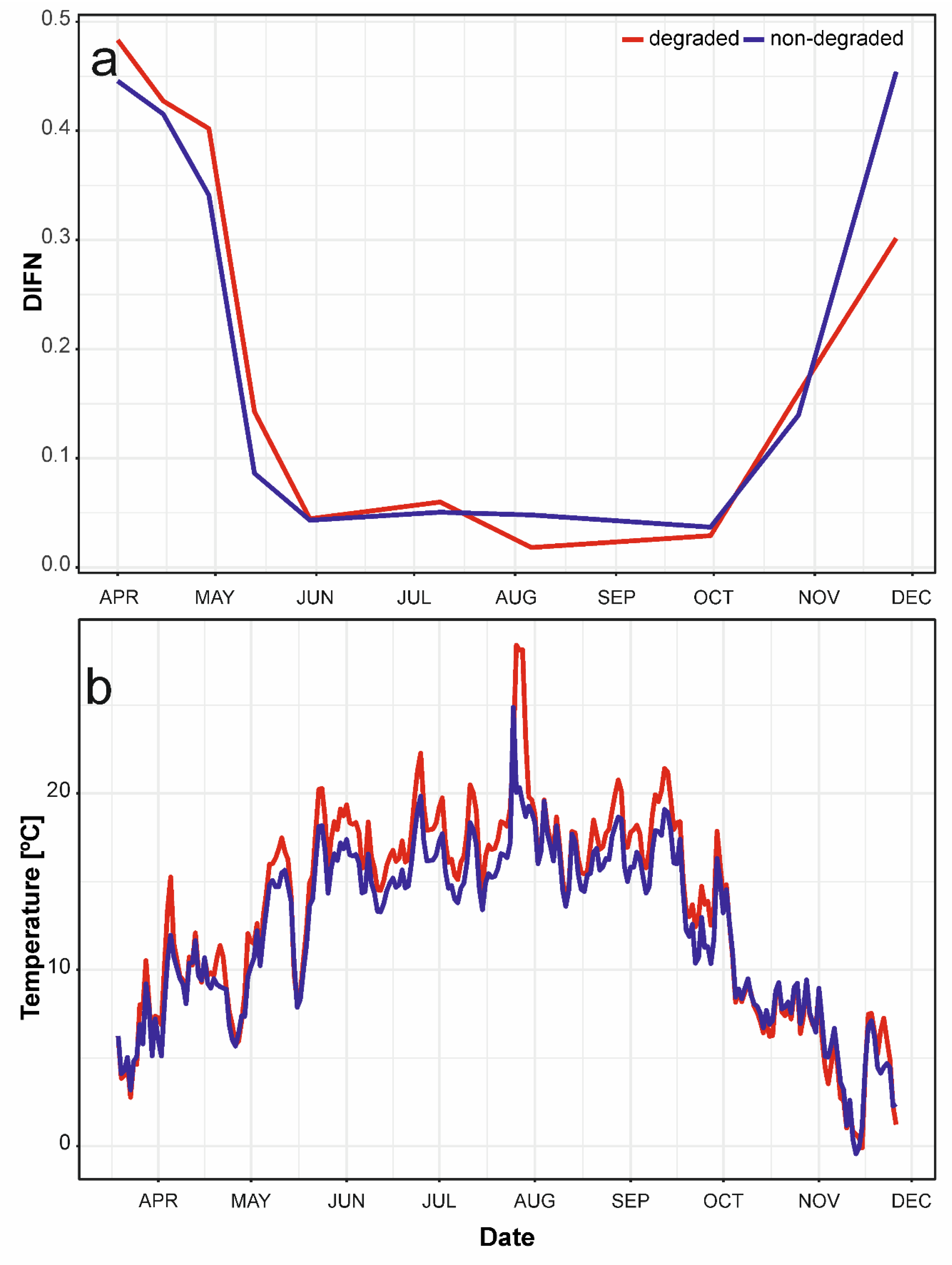
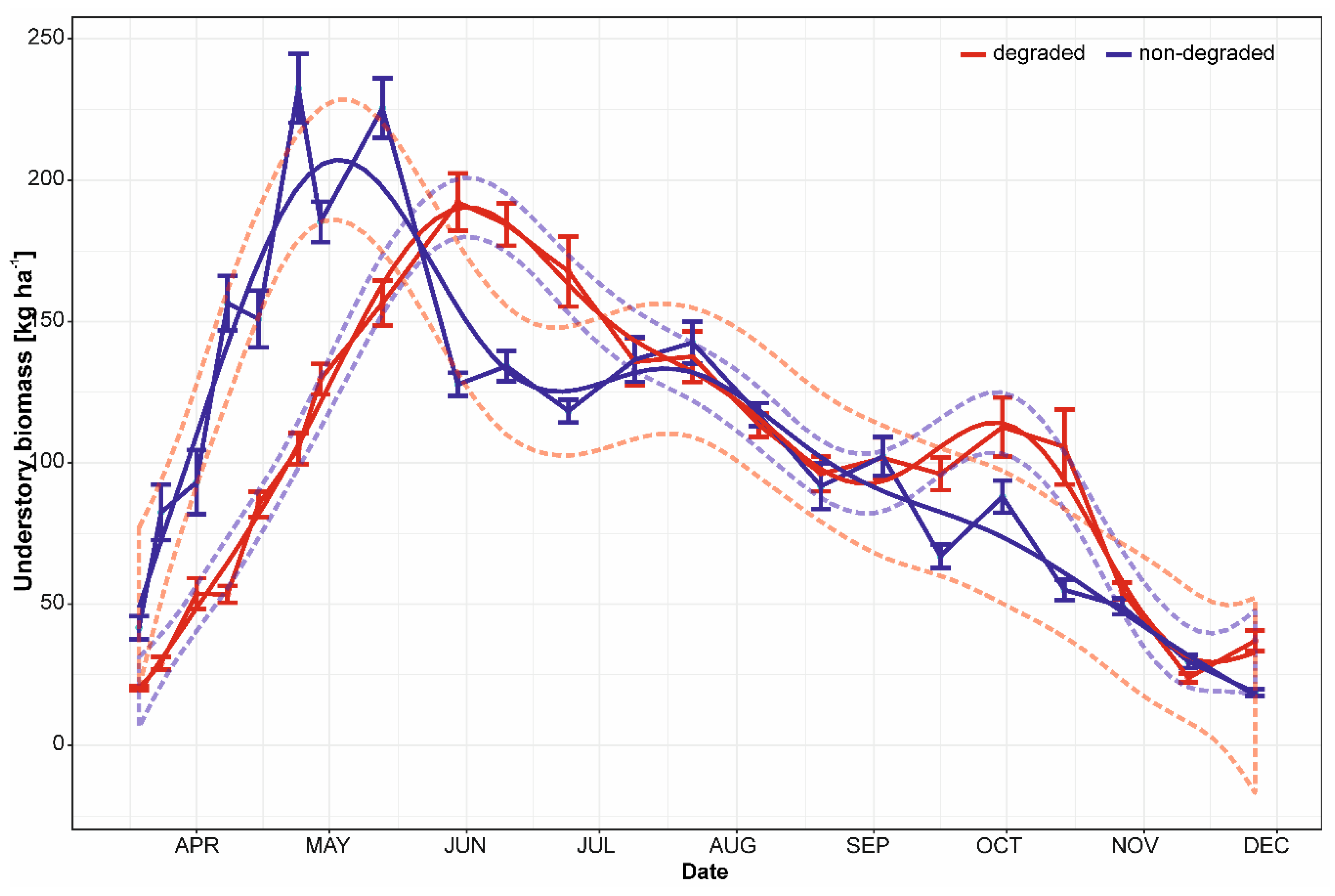
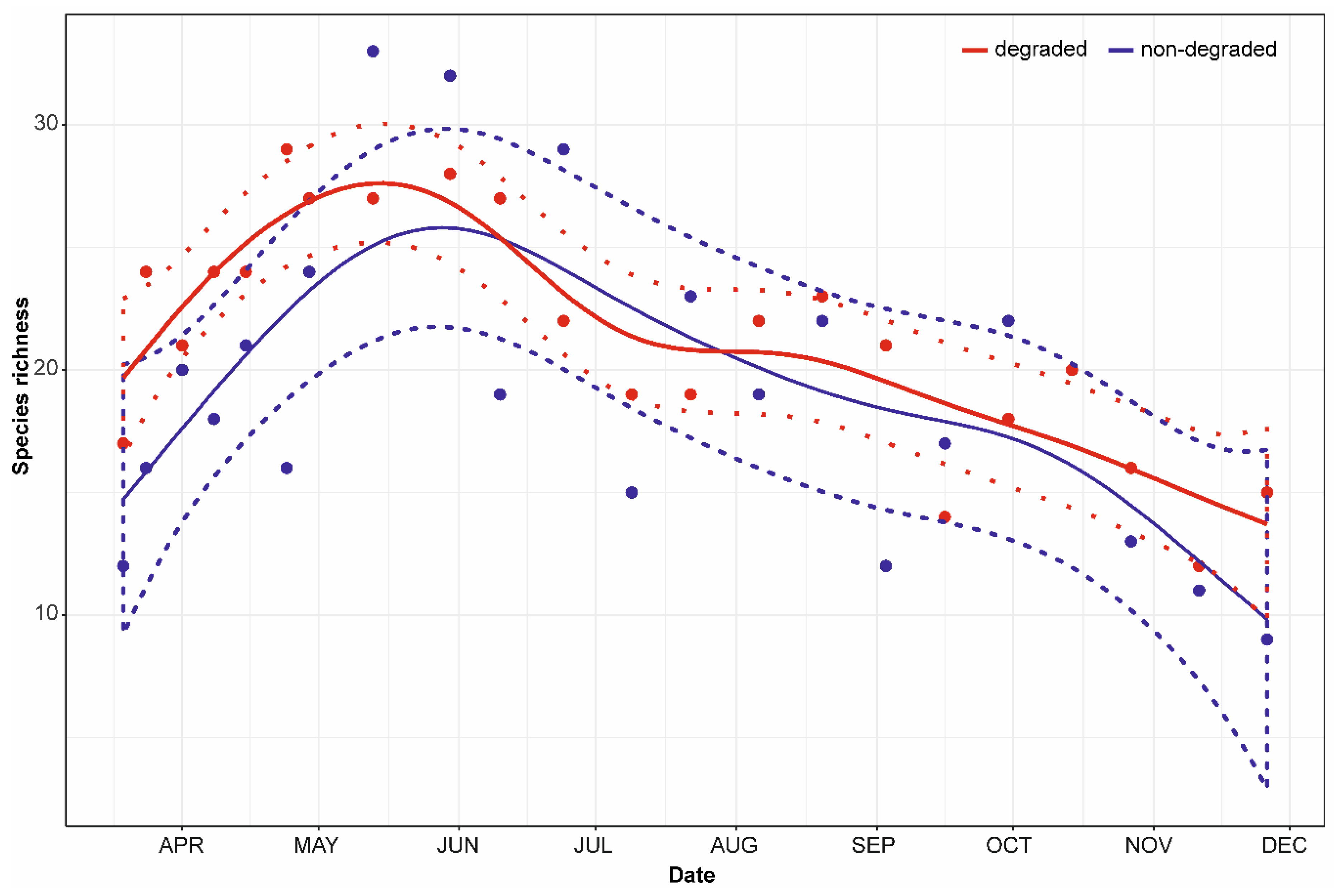
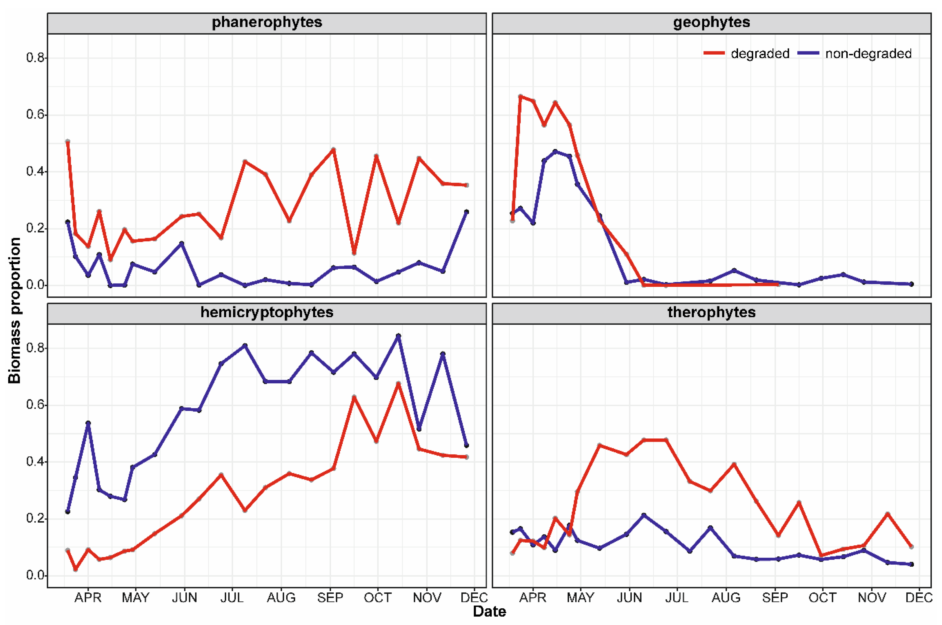
3. Results
3.1. Seasonal Dynamics of Biomass
3.2. Dynamics of Species Richness
3.3. Dynamics of Life Form Proportions
3.4. Impact of Environmental Factors on Understory Biomass Species Composition Dynamics.
4. Discussion
4.1. Limitations of the Study
4.2. Biomass Crop and Its Change over Growing Season
4.3. Differences between Non-Degraded and Degraded Floodplain Forest
4.4. Dynamics of Life-Forms Proportions
5. Conclusions
Supplementary Materials
Author Contributions
Funding
Acknowledgments
Conflicts of Interest
References
- Hood, W.G.; Naiman, R.J. Vulnerability of riparian zones to invasion by exotic vascular plants. Plant Ecol. 2000, 148, 105–114. [Google Scholar] [CrossRef]
- Richardson, D.M.; Holmes, P.M.; Esler, K.J.; Galatowitsch, S.M.; Stromberg, J.C.; Kirkman, S.P.; Pyšek, P.; Hobbs, R.J. Riparian vegetation: Degradation, alien plant invasions, and restoration prospects. Divers. Distrib. 2007, 13, 126–139. [Google Scholar] [CrossRef]
- Tabacchi, E.; Planty-Tabacchi, A.-M.; Salinas, M.J.; Décamps, H. Landscape Structure and Diversity in Riparian Plant Communities: A Longitudinal Comparative Study. Reg. Rivers: Res. Manag. 1996, 12, 367–390. [Google Scholar] [CrossRef]
- Dyderski, M.K.; Gdula, A.K.; Jagodziński, A.M. “The rich get richer” concept in riparian woody species—A case study of the Warta River Valley (Poznań, Poland). Urban For. Urban Green. 2015, 14, 107–114. [Google Scholar] [CrossRef]
- Pielech, R. Formalised classification and environmental controls of riparian forest communities in the Sudetes (SW Poland). Tuexenia 2015, 155–176. [Google Scholar]
- Olden, J.D.; LeRoy Poff, N.; Douglas, M.R.; Douglas, M.E.; Fausch, K.D. Ecological and evolutionary consequences of biotic homogenization. Trends Ecol. Evol. 2004, 19, 18–24. [Google Scholar] [CrossRef] [PubMed]
- Chen, H.; Qian, H.; Spyreas, G.; Crossland, M. Native-exotic species richness relationships across spatial scales and biotic homogenization in wetland plant communities of Illinois, USA. Divers. Distrib. 2010, 16, 737–743. [Google Scholar] [CrossRef]
- Brice, M.-H.; Pellerin, S.; Poulin, M. Does urbanization lead to taxonomic and functional homogenization in riparian forests? Divers. Distrib. 2017, 23, 828–840. [Google Scholar] [CrossRef]
- Mortenson, S.G.; Weisberg, P.J. Does river regulation increase the dominance of invasive woody species in riparian landscapes? Glob. Ecol. Biogeogr. 2010, 19, 562–574. [Google Scholar] [CrossRef]
- Catford, J.A.; Downes, B.J.; Gippel, C.J.; Vesk, P.A. Flow regulation reduces native plant cover and facilitates exotic invasion in riparian wetlands. J. Appl. Ecol 2011, 48, 432–442. [Google Scholar] [CrossRef]
- Chocholoušková, Z.; Pyšek, P. Changes in composition and structure of urban flora over 120 years: A case study of the city of Plzeň. Flora 2003, 198, 366–376. [Google Scholar] [CrossRef]
- Knapp, S.; Kühn, I.; Stolle, J.; Klotz, S. Changes in the functional composition of a Central European urban flora over three centuries. Persp. Plant Ecol. Evol. System. 2010, 12, 235–244. [Google Scholar] [CrossRef]
- Jarošík, V.; Pyšek, P.; Kadlec, T. Alien plants in urban nature reserves: From red-list species to future invaders? NeoBiota 2011, 10, 27–46. [Google Scholar] [CrossRef]
- Nilsson, C.; Reidy, C.A.; Dynesius, M.; Revenga, C. Fragmentation and Flow Regulation of the World’s Large River Systems. Science 2005, 308, 405–408. [Google Scholar] [CrossRef] [PubMed]
- Kowarik, I. Novel urban ecosystems, biodiversity, and conservation. Environm. Poll. 2011, 159, 1974–1983. [Google Scholar] [CrossRef]
- Swan, C.M.; Pickett, S.T.A.; Szlavecz, K.; Warren, P.; Willey, K.T. Biodiversity and Community Composition in Urban Ecosystems: Coupled Human, Spatial, and Metacommunity Processes. In Urban Ecology; Breuste, J.H., Elmqvist, T., Guntenspergen, G., James, P., McIntyre, N.E., Eds.; Oxford University Press: Oxford, UK, 2011; pp. 179–186. ISBN 978-0-19-956356-2. [Google Scholar]
- Dyderski, M.K.; Wrońska-Pilarek, D.; Jagodziński, A.M. Ecological lands for conservation of vascular plant diversity in the urban environment. Urban Ecosyst. 2016, 1–12. [Google Scholar] [CrossRef]
- Pyšek, P.; Prach, K. Plant Invasions and the Role of Riparian Habitats: A Comparison of Four Species Alien to Central Europe. J. Biogeogr. 1993, 20, 413–420. [Google Scholar] [CrossRef]
- Dyderski, M.K.; Jagodziński, A.M. Patterns of plant invasions at small spatial scale correspond with that at the whole country scale. Urban Ecosyst. 2016, 19, 983–998. [Google Scholar] [CrossRef]
- Pergl, J.; Sádlo, J.; Petřík, P.; Danihelka, J.; Chrtek Jr, J.; Hejda, M.; Moravcova, L.; Perglová, I.; Štajerová, K.; Pyšek, P. Dark side of the fence: Ornamental plants as a source of wild-growing flora in the Czech Republic. Preslia 2016, 88, 163–184. [Google Scholar]
- Turner, D.P.; Koerper, G.J.; Harmon, M.E.; Lee, J.J. A Carbon Budget for Forests of the Conterminous United States. Ecol. Appl. 1995, 5, 421–436. [Google Scholar] [CrossRef]
- Yarie, J. The Role of Understory Vegetation in the Nutrient Cycle of Forested Ecosystems in the Mountain Hemlock Biogeoclimatic Zone. Ecology 1980, 61, 1498–1514. [Google Scholar] [CrossRef]
- Gilliam, F.S. The ecological significance of the herbaceous layer in temperate forest ecosystems. Bioscience 2007, 57, 845–858. [Google Scholar] [CrossRef]
- Muller, R.N. Nutrient Relations of the Herbaceous Layer in Deciduous Forest Ecosystems. In The Herbaceous Layer in Forests of Eastern North America; Gilliam, F., Ed.; Oxford University Press: Oxford, UK, 2014; pp. 12–34. ISBN 978-0-19-983765-6. [Google Scholar]
- Small, C.J.; McCarthy, B.C. Spatial and temporal variability of herbaceous vegetation in an eastern deciduous forest. Plant Ecol. 2003, 164, 37–48. [Google Scholar] [CrossRef]
- Jagodziński, A.M.; Dyderski, M.K.; Rawlik, K.; Kątna, B. Seasonal variability of biomass, total leaf area and specific leaf area of forest understory herbs reflects their life strategies. For. Ecol. Manag. 2016, 374, 71–81. [Google Scholar] [CrossRef]
- Jagodziński, A.M.; Pietrusiak, K.; Rawlik, M.; Janyszek, S. Seasonal changes in the understorey biomass of an oak-hornbeam forest Galio sylvatici-Carpinetum betuli. For. Res. Pap. 2013, 74, 35–47. [Google Scholar] [CrossRef]
- Rawlik, M.; Jagodzinski, A.M.; Janyszek, S. Seasonal changes in the understorey biomass of an oak-hornbeam forest Stellario holosteae-Carpinetum betuli. For. Res. Pap. 2012, 73, 221–235. [Google Scholar] [CrossRef]
- Lapointe, L. How phenology influences physiology in deciduous forest spring ephemerals. Physiol. Plant. 2001, 113, 151–157. [Google Scholar] [CrossRef]
- Rothstein, D.E.; Zak, D.R. Photosynthetic adaptation and acclimation to exploit seasonal periods of direct irradiance in three temperate, deciduous-forest herbs. Funct. Ecol. 2001, 15, 722–731. [Google Scholar] [CrossRef]
- Mueller, K.E.; Eisenhauer, N.; Reich, P.B.; Hobbie, S.E.; Chadwick, O.A.; Chorover, J.; Dobies, T.; Hale, C.M.; Jagodziński, A.M.; Kałucka, I.; et al. Light, earthworms, and soil resources as predictors of diversity of 10 soil invertebrate groups across monocultures of 14 tree species. Soil Biol. Biochem. 2016, 92, 184–198. [Google Scholar] [CrossRef]
- Augspurger, C.K.; Salk, C.F. Constraints of cold and shade on the phenology of spring ephemeral herb species. J. Ecol. 2017, 105, 246–254. [Google Scholar] [CrossRef]
- Barbier, S.; Gosselin, F.; Balandier, P. Influence of tree species on understory vegetation diversity and mechanisms involved–A critical review for temperate and boreal forests. For. Ecol. Manag. 2008, 254, 1–15. [Google Scholar] [CrossRef]
- Jagodziński, A.M.; Oleksyn, J. Ekologiczne konsekwencje hodowli drzew w różnym zagęszczeniu. II. Produkcja i alokacja biomasy, retencja biogenów. Sylwan 2009, 3, 147–157. [Google Scholar]
- Ampoorter, E.; Baeten, L.; Vanhellemont, M.; Bruelheide, H.; Scherer-Lorenzen, M.; Baasch, A.; Erfmeier, A.; Hock, M.; Verheyen, K. Disentangling tree species identity and richness effects on the herb layer: First results from a German tree diversity experiment. J. Veg. Sci. 2015, 26, 742–755. [Google Scholar] [CrossRef]
- Fortier, J.; Truax, B.; Gagnon, D.; Lambert, F. Biomass carbon, nitrogen and phosphorus stocks in hybrid poplar buffers, herbaceous buffers and natural woodlots in the riparian zone on agricultural land. J. Environ. Manag. 2015, 154, 333–345. [Google Scholar] [CrossRef] [PubMed]
- Rawlik, M.; Kasprowicz, M.; Jagodzinski, A.M. Differentiation of herb layer vascular flora in reclaimed areas depends on the species composition of forest stands. For. Ecol. Manag. 2018, 409, 541–551. [Google Scholar] [CrossRef]
- Axmanová, I.; Chytrý, M.; Zelený, D.; Li, C.-F.; Vymazalová, M.; Danihelka, J.; Horsák, M.; Kočí, M.; Kubešová, S.; Lososová, Z.; et al. The species richness–productivity relationship in the herb layer of European deciduous forests. Glob. Ecol. Biogeogr. 2012, 21, 657–667. [Google Scholar] [CrossRef]
- Woziwoda, B.; Parzych, A.; Kopeć, D. Species diversity, biomass accumulation and carbon sequestration in the understorey of post-agricultural Scots pine forests. Silva Fenn. 2014, 48, 1119. [Google Scholar] [CrossRef]
- Ruffing, C.M.; Dwire, K.A.; Daniels, M.D. Carbon pools in stream-riparian corridors: Legacy of disturbance along mountain streams of south-eastern Wyoming. Earth Surf. Process. Landf. 2016, 41, 208–223. [Google Scholar] [CrossRef]
- Tremblay, N.O.; Larocque, G.R. Seasonal dynamics of understory vegetation in four eastern Canadian forest types. Int. J. Plant Sci. 2001, 162, 271–286. [Google Scholar] [CrossRef]
- Nilsson, C.; Berggren, K. Alterations of Riparian Ecosystems Caused by River Regulation Dam operations have caused global-scale ecological changes in riparian ecosystems. How to protect river environments and human needs of rivers remains one of the most important questions of our time. BioScience 2000, 50, 783–792. [Google Scholar] [CrossRef]
- Tabacchi, E.; Planty-Tabacchi, A.-M. Recent changes in riparian vegetation: Possible consequences on dead wood processing along rivers. River Res. Appl. 2003, 19, 251–263. [Google Scholar] [CrossRef]
- Mölder, A.; Schneider, E. On the beautiful diverse Danube? Danubian floodplain forest vegetation and flora under the influence of river eutrophication. River Res. Appl. 2011, 27, 881–894. [Google Scholar] [CrossRef]
- Douda, J.; Boublík, K.; Slezák, M.; Biurrun, I.; Nociar, J.; Havrdová, A.; Doudová, J.; Aćić, S.; Brisse, H.; Brunet, J.; et al. Vegetation classification and biogeography of European floodplain forests and Alder Carrs. Appl. Veg. Sci. 2016, 19, 147–163. [Google Scholar] [CrossRef]
- Britson, A.; Wardrop, D.; Drohan, P. Plant community composition as a driver of decomposition dynamics in riparian wetlands. Wetl. Ecol. Manag. 2016, 24, 335–346. [Google Scholar] [CrossRef]
- Xiu, C.; Gerisch, M.; Ilg, C.; Henle, K.; Ouyang, Z. Effects of hydrologic modifications to riparian plant communities in a large river system in northern China. Ecol. Res. 2015, 30, 461–469. [Google Scholar] [CrossRef]
- White, D.A.; Visser, J.M. Water quality change in the Mississippi River, including a warming river, explains decades of wetland plant biomass change within its Balize delta. Aquat. Bot. 2016, 132, 5–11. [Google Scholar] [CrossRef]
- Zelarayán, M.L.C.; Celentano, D.; Oliveira, E.C.; Triana, S.P.; Sodré, D.N.; Muchavisoy, K.H.M.; Rousseau, G.X.; Zelarayán, M.L.C.; Celentano, D.; Oliveira, E.C.; et al. Impacto da degradação sobre o estoque total de carbono de florestas ripárias na Amazônia Oriental, Brasil. Acta Amaz. 2015, 45, 271–282. [Google Scholar] [CrossRef]
- Mabry, C.M.; Gerken, M.E.; Thompson, J.R. Seasonal storage of nutrients by perennial herbaceous species in undisturbed and disturbed deciduous hardwood forests. Appl. Veg. Sci. 2008, 11, 37–44. [Google Scholar] [CrossRef]
- Dunham, K.M. Biomass dynamics of herbaceous vegetation in Zambezi riverine woodlands. Afr. J. Ecol. 1990, 28, 200–212. [Google Scholar] [CrossRef]
- Wilson, K.B.; Baldocchi, D.D.; Hanson, P.J. Spatial and seasonal variability of photosynthetic parameters and their relationship to leaf nitrogen in a deciduous forest. Tree Physiol. 2000, 20, 565–578. [Google Scholar] [CrossRef]
- Poznań. Rocznik Statystyczny Poznania; Urząd Statystyczny w Poznaniu: Poznań, Poland, 2013.
- Jackowiak, B. Plants and Habitats of European Cities; Müller, N., Kelcey, J.G., Eds.; Springer: New York, NY, USA, 2011; pp. 363–405. ISBN 978-0-387-89683-0. [Google Scholar]
- Ellenberg, H. Vegetation Ecology of Central Europe; Cambridge University Press: Cambridge, UK, 1988; ISBN 978-0-521-23642-3. [Google Scholar]
- Anderson-Teixeira, K.J.; Davies, S.J.; Bennett, A.C.; Gonzalez-Akre, E.B.; Muller-Landau, H.C.; Wright, S.J.; Salim, K.A.; Zambrano, A.M.A.; Alonso, A.; Baltzer, J.L.; et al. CTFS-ForestGEO: A worldwide network monitoring forests in an era of global change. Glob. Change Biol. 2015, 21, 528–549. [Google Scholar] [CrossRef] [PubMed]
- McMahon, S.M.; Parker, G.G. A general model of intra-annual tree growth using dendrometer bands. Ecol. Evol. 2015, 5, 243–254. [Google Scholar] [CrossRef] [PubMed]
- Dyderski, M.K.; Jagodziński, A.M. Drivers of invasive tree and shrub natural regeneration in temperate forests. Biol. Invasions 2018, 20, 2363–2379. [Google Scholar] [CrossRef]
- Ellenberg, H.; Leuschner, C. Vegetation Mitteleuropas Mit Den Alpen in Ökologischer, Dynamischer und Historischer Sicht; UTB: Stuttgart, Germany, 2010. [Google Scholar]
- Klotz, S.; Kühn, I.; Durka, W. BIOLFLOR–Eine Datenbank zu Biologisch-Ökologischen Merkmalen der Gefäßpflanzen in Deutschland. Schriftenreihe für Vegetationskunde; Schriftenreihe für Vegetationskunde; Bundesamt für Naturschutz: Bonn, Germany, 2002. [Google Scholar]
- Wood, S.N. Fast stable restricted maximum likelihood and marginal likelihood estimation of semiparametric generalized linear models. J. R. Stat. Soc. Ser. B 2011, 73, 3–36. [Google Scholar] [CrossRef]
- Oksanen, J.; Blanchet, F.G.; Kindt, R.; Legendre, P.; Michin, P.R.; O’Hara, R.B.; Simpson, G.L.; Solymos, P.; Henry, M.; Stevens, H.; et al. “vegan” 2.3.3.-Community Ecology Package. Available online: https://cran.r-project.org/web/packages/vegan/index.html (accessed on 21 December 2018).
- R Core Team R: A Language and Environment for Statistical Computing; R Foundation for Statistical Computing: Vienna, Austria, 2018.
- Parker, G.G.; Harmon, M.E.; Lefsky, M.A.; Chen, J.; Van Pelt, R.; Weiss, S.B.; Thomas, S.C.; Winner, W.E.; Shaw, D.C.; Franklin, J.F. Three dimensional structure of an old-growth Pseudotsuga-Tsuga canopy and its implications for radiation balance, microclimate, and atmoshperic gas exchange. Ecosystems 2004, 7, 440–453. [Google Scholar] [CrossRef]
- Araujo Calçada, E.; Closset-Kopp, D.; Lenoir, J.; Hermy, M.; Decocq, G. Site productivity overrides competition in explaining the disturbance–diversity relationship in riparian forests. Perspect. Plant Ecol. Evol. Syst. 2015, 17, 434–443. [Google Scholar] [CrossRef]
- Knight, K.S.; Oleksyn, J.; Jagodzinski, A.M.; Reich, P.B.; Kasprowicz, M. Overstorey tree species regulate colonization by native and exotic plants: A source of positive relationships between understorey diversity and invasibility. Divers. Distrib. 2008, 14, 666–675. [Google Scholar] [CrossRef]
- Von Arx, G.; Dobbertin, M.; Rebetez, M. Spatio-temporal effects of forest canopy on understory microclimate in a long-term experiment in Switzerland. Agric. For. Meteorol. 2012, 166–167, 144–155. [Google Scholar] [CrossRef]
- Kaźmierczakowa, R. Ekologia i produkcja runa świetlistej dąbrowy i grądu w rezerwatach Kwiatówka i Lipny Dół na Wyżynie Małopolskiej. Stud. Nat. 1971, 5, 1–98. [Google Scholar]
- Chmura, D. Charakterystyka fitocenotyczna leśnych zbiorowisk zastępczych z udziałem Quercus rubra L. na Wyżynie Śląskiej. Acta Bot. Siles. 2014, 10, 17–40. [Google Scholar]
- Chmura, D. Penetration and naturalisation of invasive alien plant species (neophytes) in woodlands of the Silesian Upland (southern Poland). Nat. Conserv. 2004, 60, 3–11. [Google Scholar]
- Wagner, V.; Chytrý, M.; Jiménez-Alfaro, B.; Pergl, J.; Hennekens, S.; Biurrun, I.; Knollová, I.; Berg, C.; Vassilev, K.; Rodwell, J.S.; et al. Alien plant invasions in European woodlands. Divers. Distrib. 2017, 23, 969–981. [Google Scholar] [CrossRef]
- Peace, W.J.H.; Grubb, P.J. Interaction of Light and Mineral Nutrient Supply in the Growth of Impatiens parviflora. New Phytol. 1982, 90, 127–150. [Google Scholar] [CrossRef]
- Piskorz, R. The effect of oak-hornbeam diversity on flowering and fruiting of Impatiens parviflora DC. Roczniki Akademii Rolniczej w Poznaniu–Botanica Steciana 2005, 373, 187–196. [Google Scholar]
- Gerken Golay, M.; Thompson, J.; Kolka, R. Carbon, nitrogen and phosphorus storage across a growing season by the herbaceous layer in urban and preserved temperate hardwood forests. Appl. Veg. Sci. 2016, 19, 689–699. [Google Scholar] [CrossRef]


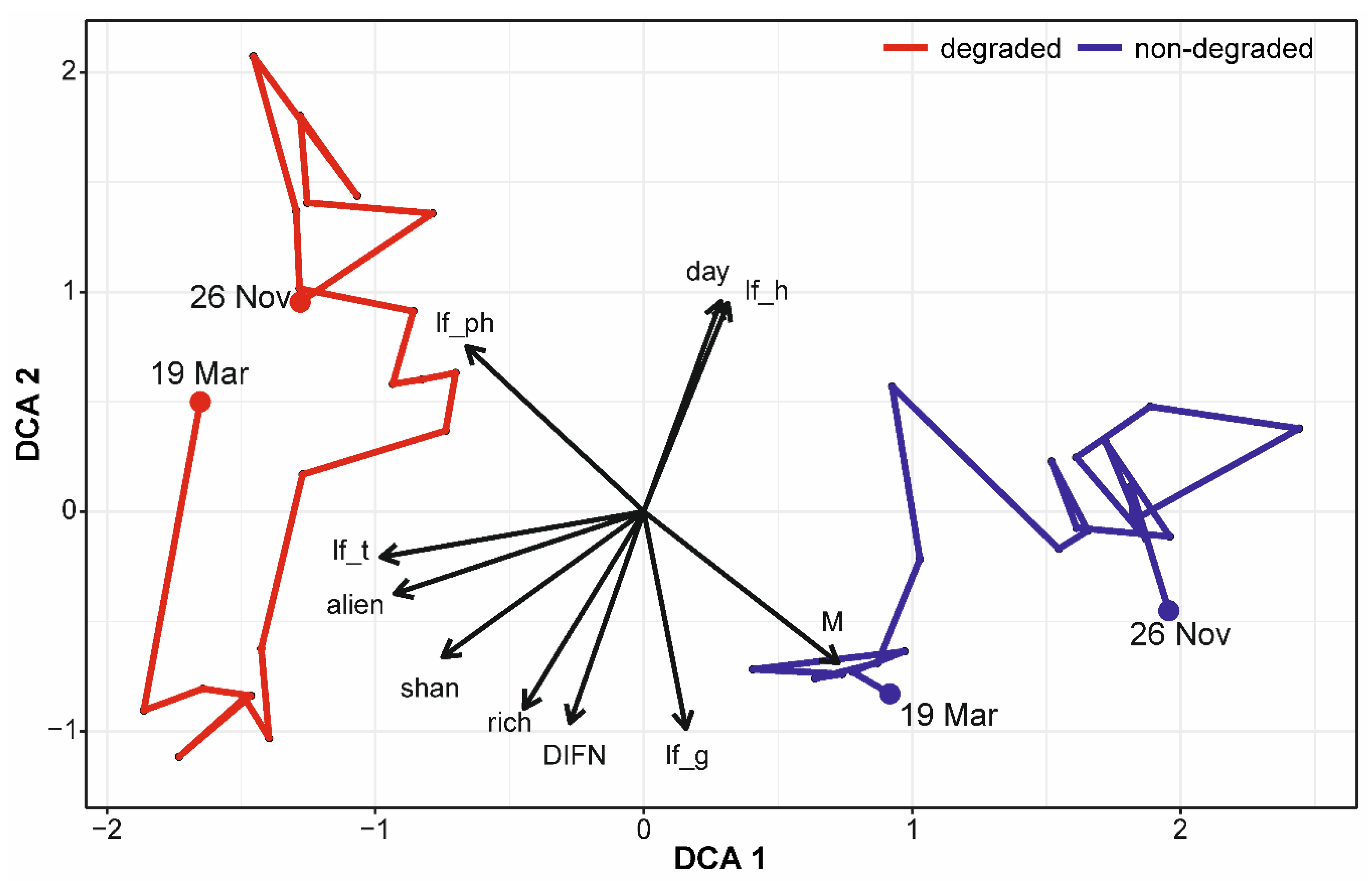
| Parameter | Abbreviation | DCA1 | DCA2 | R2 | p |
|---|---|---|---|---|---|
| Day in year | day | 0.28602 | 0.95822 | 0.6060 | 0.001 |
| Temperature | temp | 0.07346 | 0.99730 | 0.1524 | 0.065 |
| DIFN | DIFN | −0.27537 | −0.96134 | 0.4247 | 0.001 |
| Proportion of life forms | |||||
| - phanerophytes | lf_ph | −0.65970 | 0.75153 | 0.6717 | 0.001 |
| - geophytes | lf_g | 0.15727 | −0.98756 | 0.7070 | 0.001 |
| - hemicryptophytes | lf_h | 0.31312 | 0.94971 | 0.7278 | 0.001 |
| - therophytes | lf_t | −0.97844 | −0.20653 | 0.3683 | 0.002 |
| Ellennberg’s ecological indicator values | |||||
| - soil fertility | N | 0.74511 | 0.66694 | 0.0876 | 0.216 |
| - moisture | M | 0.72399 | −0.68981 | 0.6979 | 0.001 |
| - soil reaction | SR | 0.27500 | −0.96144 | 0.0473 | 0.466 |
| Shannon diversity index | shan | −0.74938 | −0.66214 | 0.4589 | 0.001 |
| Species richness | rich | −0.44518 | −0.89544 | 0.2129 | 0.023 |
| Proportion of alien species | alien | −0.92770 | −0.37331 | 0.3378 | 0.002 |
| Parameter | Estimate | SE | t Value | Pr (>|t|) |
|---|---|---|---|---|
| (Intercept) | −349.930 | 241.110 | −1.451 | 0.155 |
| mean temperature of previous two weeks | 43.860 | 12.190 | 3.597 | 0.001 |
| DIFN2 | −5155.920 | 2373.290 | −2.172 | 0.036 |
| DIFN | 3158.170 | 1322.740 | 2.388 | 0.022 |
© 2019 by the authors. Licensee MDPI, Basel, Switzerland. This article is an open access article distributed under the terms and conditions of the Creative Commons Attribution (CC BY) license (http://creativecommons.org/licenses/by/4.0/).
Share and Cite
Czapiewska, N.; Dyderski, M.K.; Jagodziński, A.M. Seasonal Dynamics of Floodplain Forest Understory–Impacts of Degradation, Light Availability and Temperature on Biomass and Species Composition. Forests 2019, 10, 22. https://doi.org/10.3390/f10010022
Czapiewska N, Dyderski MK, Jagodziński AM. Seasonal Dynamics of Floodplain Forest Understory–Impacts of Degradation, Light Availability and Temperature on Biomass and Species Composition. Forests. 2019; 10(1):22. https://doi.org/10.3390/f10010022
Chicago/Turabian StyleCzapiewska, Natalia, Marcin K. Dyderski, and Andrzej M. Jagodziński. 2019. "Seasonal Dynamics of Floodplain Forest Understory–Impacts of Degradation, Light Availability and Temperature on Biomass and Species Composition" Forests 10, no. 1: 22. https://doi.org/10.3390/f10010022
APA StyleCzapiewska, N., Dyderski, M. K., & Jagodziński, A. M. (2019). Seasonal Dynamics of Floodplain Forest Understory–Impacts of Degradation, Light Availability and Temperature on Biomass and Species Composition. Forests, 10(1), 22. https://doi.org/10.3390/f10010022