Changes in Soil Hydro-Physical Properties and SOM Due to Pine Afforestation and Grazing in Andean Environments Cannot Be Generalized

Abstract

Andean ecosystems provide important ecosystem services including streamflow regulation and carbon sequestration, services that are controlled by the water retention properties of the soils. Even though these soils have been historically altered by pine afforestation and grazing, little research has been dedicated to the assessment of such impacts at local or regional scales. To partially fill this knowledge gap, we present an evaluation of the impacts of pine plantations and grazing on the soil hydro-physical properties and soil organic matter (SOM) of high montane forests and páramo in southern Ecuador, at elevations varying between 2705 and 3766 m a.s.l. In total, seven study sites were selected and each one was parceled into undisturbed and altered plots with pine plantation and grazing. Soil properties were characterized at two depths, 0–10 and 10–25 cm, and differences in soil parameters between undisturbed and disturbed plots were analyzed versus factors such as ecosystem type, sampling depth, soil type, elevation, and past/present land management. The main soil properties affected by land use change are the saturated hydraulic conductivity (K_sat), the water retention capacity (pF 0 to 2.52), and SOM. The impacts of pine afforestation are dependent on sampling depth, ecosystem type, plantation characteristics, and previous land use, while the impacts of grazing are primarily dependent on sampling depth and land use management (grazing intensity and tilling activities). The site-specific nature of the found relations suggests that extension of findings in response to changes in land use in montane Andean ecosystems is risky; therefore, future evaluations of the impact of land use change on soil parameters should take into consideration that responses are or can be site specific.

1. Introduction

High montane forests and páramo [1], typical Andean ecosystems, provide important services such as water supply regulation and carbon storage [2]. The hydrological services provided by Andean ecosystems have been closely related to the characteristic functions played by their soils at watershed scale [3,4,5]. These characteristics include: high soil organic matter (SOM) content [6], overall low bulk density (BD) (<0.6 g cm⁻³) [7], and high-water retention capacity [7,8,9,10,11,12]. Despite the important role soils play with respect to the provision of ecosystem services in the Andean region, they have been increasingly altered by anthropogenic activities since pre-Hispanic times [13], and only a limited number of evaluations of the effects of anthropogenic land-use changes on soil properties exist.

In the Andean region, afforestation and grazing are the main anthropogenic activities affecting montane ecosystems [12,14,15,16]. Afforestation, primarily with pine, has been carried out to produce timber and reduce pressure on native ecosystems [16,17,18,19], as well as to capture carbon [19,20,21]. Without focus on the possible impact on soil and water resources, the majority of pine plantations were established on sites of important hydrological and ecological value to the Andean population. Grazing in the montane Andean ecosystems has been carried out since pre-Hispanic times (XV century), and this practice results mainly from extensive to intensive animal farming (cattle, horses, and sheep) [13]. In some cases, grazing is carried out directly in natural cover, considering tussock grass as fodder, or after burning to convert the land, whether or not accompanied with the introduction of more productive grass species [22], into suitable pasture where cattle can obtain more nutritious fodder [18].

Pine plantations and grazing interventions in Andean ecosystems have led to significant changes in the hydro-physical properties and SOM content, in particular of the top soil at depths lower than 30 cm [19,20,23,24]. Modifications in soil properties are causal factors of a reduction in water yield and variations in the hydrological response of montane Andean basins [25,26]. In the case of pine afforestation, the soils tend to dry out because of the high water absorption capacity of the trees, which favors SOM decomposition [19,20] and reduces the soil’s water retention capacity [15]. Furthermore, preferential flows created by root growth increase the saturated hydraulic conductivity (K_sat) of soils [27]. Despite existing investigations, there still exists indistinctness and contradictions about the effect of anthropogenic impacts, such as pine plantations and grazing, on the soil properties of Andean ecosystems [28]. Some studies reported an increment in SOM in the Andosols of pine plantations [28], while other studies found no evidence of changes [29]. Additionally, in most studies, important factors capable of influencing changes in soil hydro-physical properties, such as previous land-use practices as evidenced by La Manna et al. [30], have not been considered. Similarly, the effects of livestock grazing, whether or not accompanied by burning, have been interpreted in different ways. Some authors claim that greater solar radiation exposure leads to soil drought, an increase in BD, SOM loss [19,23,31], and a reduction in soil water retention [23,32]; while a reduction of K_sat enhances water erosion [28]. Despite previous findings, under grazing activities some authors have shown, probably due to pre-tilling activities, a reduction in the BD and an increment in SOM [28,33]. Such discrepancies could be due to the intensity of grazing. In some cases, extensive grazing is not considered a source of stress on high Andean ecosystems [34].

Considering the role of soil properties in the provision of ecosystem services in Ecuador’s Andean environments, and the past and present anthropogenic pressures resulting from afforestation and grazing activities, the main objective of this study was to evaluate the impact of pine afforestation and grazing on the hydro-physical properties and SOM content of the surface horizons of high montane forest and páramo soils. The study was guided by the following research hypotheses: (1) to properly assess anthropogenic impacts it is recommended to collect information of unaltered and altered plots on neighboring comparable sites to avoid that interpretation of results is biased by local site differences and (2) the impact of land-use change on the hydro-physical soil properties is not unique and often masked by other factors such as antecedent land-use, spatial variability, texture, elevation, climate, among other site-specific factors. The evaluation of both these hypotheses will not only improve the research quality and the capability to generalize research findings, but also the effectiveness of future decision making and conservation policies of high-elevation ecosystems in the Andean region.

2. Materials and Methods

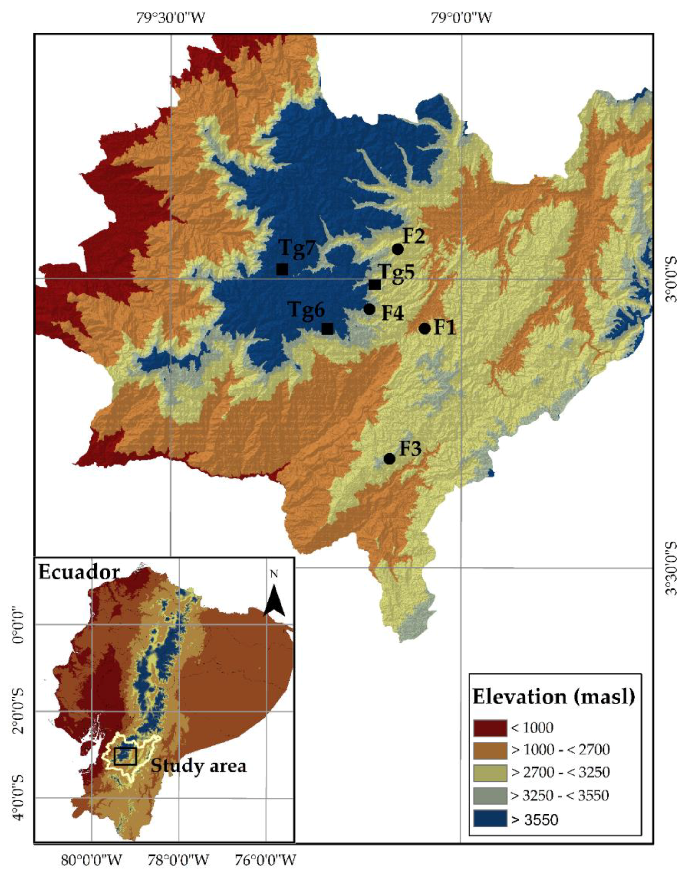
2.1. Study Area

The study was conducted in the province of Azuay, southern Ecuador, in an area whose elevation varies between 2705 and 3766 m above sea level (a.s.l.) (Figure 1). The area is dominated by two Andean montane ecosystems—high montane forest and páramo. The high montane forest consists of evergreen vegetation with an arboreal stratum between 3 and 10 m tall, a great variety of vegetation and a high epiphyte density [35,36]. The predominant species there belong to the Solanaceae, Melastomataceae, Rosaceae, Ericaceae, Chlorantaceae, Myrtaceae, Lauraceae and Podocarpaceae families [8]. The páramo comprises predominantly herbaceous shrub-type vegetation (Calamagrostis intermedia (J. Presl) Steud.) and cushion-like grass varieties (Azorella pedunculata (Spreng.) Mathias & Constance and Plantago rigida Kunth) [13,26,37,38].

Climate at the study area is influenced by the Pacific coast regime and the Atlantic air currents [6,39]. Average annual solar radiation varies from 11.35 to 14.5 MJ m⁻² day⁻¹, average daily temperature from 12.5 to 6 °C, and average annual precipitation from 900 to 1600 mm at elevations between 2600 and 4100 m a.s.l. [26,40]. The climate regime is bimodal with a rainy season from December to January and a less rainy season from August to September [41]. Rainfall variation is controlled by elevation and topographic parameters [12,26]. The geological material in southern Ecuador corresponds mainly to the Tarqui, Turi, and Saraguro mountain formations, which date back to the Miocene in the Neogene period. These formations are composed of a wide variety of lithological andesite rocks, ash-flow tuffs, pyroclastic flows and volcanic rocks [42].

Andosol soils of volcanic origin predominate within the study area; their depth ranges from 0.12 to >2 m [7,14,43]. Andosols are known for their Andic surface horizon (Ah), characterized by low BD [44], high porosity [11], high K_sat, and a SOM content that can exceed 40% [28,34]. This is why this horizon has a dark color, a high-water retention capacity [10,26,45], and controls to a certain extent the soil’s water regulation capacity [4]. Land use consists mainly of two anthropogenic activities: (1) afforestation with pine (Pinus patula Seem.) [14] and (2) conversion to permanent grassland (Lolium perenne L., Pennisetum clandestinum Hochst. ex Chiov. and Dactylis sp.) or in some areas grazing on burnt grasslands [15,28].

2.2. Selection and Implementation of Study Sites

Seven study sites (Figure 1) expanding between 2705 and 3766 m a.s.l. were selected at three elevation zones: (1) F1 and F2, located below 3250 m a.s.l. corresponding to the high montane forest ecosystem; (2) F3, F4, and Tg5, located between 3250 and 3550 m a.s.l. representing the transition zone between high montane forest and páramo; and (3) Tg6 and Tg7 located above 3550 m a.s.l. being occupied by páramo.

These sites were selected given that they presented intervened zones afforested with pine and converted to grass land nearby undisturbed natural cover zones, all possessing similar topographic and edaphic conditions. We considered undisturbed natural cover in high montane native forest (F) as those sites covered with tree species having a tilted growth, accompanied by a high density of epiphytes and moss, as well as leaf litter accumulation in the ground [36]. In the páramo (Tg), we considered areas with tussock grass >50 cm high and without the presence of anthropogenic intervention indicator-plants, such as Lachemilla orbiculata (Ruiz & Pav.) Rydb. [8], as undisturbed natural cover. Information was collected from pine plantations and grazing areas through field visits and interviews with the landowners [46]. At each pine plantation, the previous land-use, management, plantation age, and the slope of the land, were registered. In the case of grazing, the previous land-use, pre-tilling, and tilling activities, the slope (Sl) of the land, the age of pastures, as well as the animal load (reported as adult bovine units per hectare, ABU Ha⁻¹), were registered. A total of 17 plots with a dimension of 24 × 24 m were implemented over the 3 elevation zones, with the exception of a grazing plot in the F4 transition band between high montane forest and páramo due to the complex topographical situation, very much different from the topography of undisturbed natural cover at this elevation band. The location (geographical coordinates and elevation) and slope (Sl) of each plot, and the density or number of trees per plot (SD) were determined. The diameter at breast height (DBH), height (Ht) and canopy diameter (CD) of each tree were also measured using a tape measure and a hypsometer.

2.3. Soil Properties Characterization

A first step in the soil characterization was limited to a qualitative description of the soils in the undisturbed natural cover plots following the Food and Agriculture Organization of the United Nations-guide [47]. The qualitative description focused on the surface horizon and included measurement of the thickness, the number of roots per dm², and the structure and texture by touch. A disturbed soil sample (0.5 kg) was collected in the layer 0–10 and 10–25 cm for physical and chemical analysis. In a second prospection and sampling phase the soil hydro-physical properties and SOM content of the 0–10 and 10–25 cm surface layers of the areas with undisturbed natural cover and the areas with impacts of pine afforestation and grazing were determined. Only these two surface layers of the profile were considered since they represent the zone with highest root density and influence of tilling activities. At each surface layer of each undisturbed natural cover and grazing plot, two undisturbed soil samples (100 cm³ Kopecky rings) were randomly collected together with a disturbed sample of 0.5 kg. In the case of pine plots, the samples were taken at a distance of 75 and 150 cm from the tree trunks. The tree selection was random with a number of 3 trees per plot. At a similar density, K_sat was measured by means of the inverted auger-hole method [48] (3 repetitions per site, data shown represent the average of the repetitions). To avoid the effect on the measurement of the water-filled auger below 10 and 25 cm, respectively, the bottom of the upper and lower top layer, a plastic pipe with closed bottom was inserted in the auger holes after saturation of the soil. This enabled measuring subsequently the saturated horizontal hydraulic conductivity of both surface layers. Given the overall low bulk density of the organic top layers the soil can be considered isotropic, assuming that the vertical and horizontal saturated hydraulic conductivity are similar.

2.4. Laboratory Analyses

The disturbed samples taken during the qualitative characterization of the soil in the undisturbed natural plots were dried at room temperature (<30 °C) and passed through a 2-mm sieve. The color, pH, and SOM content were determined; the soil color was determined on wet samples using the Munsell color table. The pH was measured with a potentiometer on a 1:2.5 soil:distilled water solution [49], and the SOM content was determined through ignition of the soil at 410 °C for 16 h [50]. The BD and water retention capacity at pressure heads above field capacity were determined on undisturbed samples and are reported as pF values (or the logarithms of the negative pressure heads) corresponding to pF 0 (saturation point; pressure 1 cm H₂O), pF 0.5 (pressure 3.1 cm H₂O), pF 1.5 (31 cm H₂O) and pF 2.52 (field capacity; pressure 330 cm H₂O). Water content at saturation was considered as a proxy of porosity. Disturbed sieved soil was used for the measurement of the water retention below field capacity at pF 3.4 (2509 cm H₂O) and pF 4.2 (wilting point; 15300 cm H₂O), and the SOM content. The equipment used for the measurement of water retention was composed of sandboxes (pFs 0.5–1.5) [51] and two pressure chambers (low pressure for pF 2.52 and high pressure for pFs 3.4 and 4.2; Soilmoisture Equipment Corp., Goleta, CA, USA) [49]. Gravimetric water contents were transformed into volumetric contents. Gravitational water (GW) and water available for plants (AW) were calculated as the difference between the soil water contents at pF 0 and pF 2.52 and at pF 2.52 and pF 4.2, respectively. BD and pF at saturation were considered as proxies for soil compaction.

2.5. Statistical Analyses

For the characterization of the pine plantations and vegetation in the grazing plots and the soils in all three land uses, the median and the 25 and 75 percentiles of the distributions were defined given the lack of normality in most of the datasets as evidenced by the results of the Shapiro-Wilk test (p < 0.05). To define if elevation and differences in site as well as sampling depth have an impact on the interpretation of observations, a Spearman correlation analysis (p < 0.05) was performed between elevation, hydro-physical properties, and SOM content measured respectively at 0–10 and 10–25 cm depth under undisturbed natural cover. Subsequently, the soil properties located at the same elevation and depth were compared among the seven study sites. To this end, we applied non-parametric Kruskal-Wallis test [52] (p < 0.05) given the lack of normality in the datasets. If significant differences were identified, the Nemenyi post hoc test [53] (p < 0.05) for multiple pair comparisons was performed. The Mann-Whitney U test [54] (p < 0.05) was applied to evaluate differences in properties between the depth of 0–10 cm versus 10–25 cm.

The soil characteristics of the 0–10 and 10–25 cm soil layers of the land-use-change affected plots were compared to the same characteristics determined in the undisturbed natural cover plots to assess if the soil properties in high Andean ecosystems were affected by pine afforestation and grazing. In the pine afforested plots, first a screening was made between the properties measured at 75 and 150 cm from the trunk. The datasets were grouped if no significant differences were detected. Similarly, comparisons between the measured characteristics were made for both sampling depths (0–10 cm and 10–25 cm). Comparisons were made using the Mann-Whitney U test (p < 0.05). For a better interpretation of the impacts of afforestation, the relationship between the development of pine plantations and the soil properties was analyzed by means of the Spearman correlation analysis and linear regression (p < 0.05). Those analyses were performed on the variables of all trees with the hydro-physical soil properties and SOM content at both depths. The variables that did not present a normal distribution prior to the linear regression analysis were transformed to a normal distribution by Box-Cox method [55]. An analogue approach was followed to assess the impact of grazing. Per study site, soil characteristics at both depths at undisturbed natural cover and grazing plots were compared using the Mann-Whitney U test (p < 0.05).

To better identify and visualize the impacts of pine afforestation and grazing, forest plot graphs were built based on the differences of the medians of the pine plantations (Xtrat) vs. the undisturbed natural cover (Xcn) [56]. For grazing (Xtrat), the same procedure was followed; the differences were transformed into percentages as described by the following equation [56]:

Effects (%) = [(Xtrat − Xcn)/Xcn] × 100

(1)

Positive percentages represent an increase in the soil properties due to pine afforestation or grazing, while negative percentages represent a decrease, except for the BD. All statistical analyses were carried out by using the R program, version 3.3.2 [57].

3. Results

3.1. General Description of the Experimental Sites

In the following description of the pine afforested and grazing sites, there is always reference made to the previous land-use and/or native vegetation, as to highlight the changes introduced by respectively the introduction of pine plantation and the occupation of the land by cattle.

Table 1. General description and median values of the dendrometric variables in the pine plantations (Azuay province, southern Ecuador).

Elevation Range (m a.s.l.)	Code	Elevation (m a.s.l.)	Previous Land-Use	Sl (%)	Age (years)	SD (# of trees/plot)	DBH (cm)	Ht (m)	CD (m)	Management
<3250	F1Pi	2770	Native forest	43	29	34	25.6	19.4	5.1	Without management
	F2Pi	3260	Native forest	20	18	40	20.2	11.3	5.2	Without management
>3250–<3550	F3Pi	3359	Tussock grass subjected to equine grazing	12	17	49	18.4	8.8	5.15	Pruning
	F4Pi	3408	Tussock grasses subjected to bovine grazing	16	16	41	23.1	9.2	5	Pruning
	Tg5Pi	3485	Soils under extensive bovine grazing in burnt tussock grasses pasture.	34	21	47	16.8	8.3	3.88	Without management
>3550	Tg6Pi	3692	Tussock grass	22	19	33	8.75	4.45	1.58	Pruning
	Tg7Pi	3724	Compacted and eroded soil due to bovine grazing in burnt tussock grass	20	17.5	30	11.99	5	2.99	Without management

Legend: FxPi = pine plantation in high montane forest; TgxPi = pine plantation in the páramo; where x = 1–7 indicates sites 1–7; Sl = slope; SD = number of trees per 576 m² plot; DBH = diameter at breast height; Ht = tree height; CD = canopy diameter.

presents the general characteristics of the pine plantations in the different study sites. The F1Pi, F2Pi and Tg6Pi plantations were established on sites where previous land-use comprised native vegetation cover. The slope on those sites varied from 43 to 20, and 22%, respectively. The F3Pi, F4Pi, and Tg7Pi plantations were established on sites where extensive-grazing had taken place for more than 5 years with an animal load <1 ABU Ha⁻¹. These plantations had a slope of 12%, 16%, 34% and 20%, respectively. The majority of the plantations were 16 to 19 years old, except in the F1Pi and Tg5Pi sites where the age of the trees varied between 20 and 29 years. The number of trees per plot (SD refers to the number of trees per 576 m²) varied from 30 to 49 trees. The SD on the F1Pi, Tg6Pi, and Tg7Pi sites was smaller and varied between 30 and 34 trees. F2Pi, F3Pi, F4Pi and Tg5Pi had a greater SD (40–49 trees) (Table 1). Tree development was greater at F1Pi, F2Pi and Tg7Pi with a diameter at breast height (DBH) >18 cm, a tree height (Ht) >9 m, and a canopy diameter (CD) ≥5 m. The pine trees had slower growth in the Tg5Pi, Tg6Pi and Tg7Pi plantations, with an average DBH <18 cm, a Ht <8.5 m and a CD <5 m. In general, the management of the plantations was deficient because of the high associated costs; the F1Pi, F2Pi, Tg5Pi and Tg7Pi plantations did not receive any kind of management, while the only intervention in the F3Pi, F4Pi and Tg6Pi sites was the sporadic pruning of the trees.

Table 2. General description of the grazing sites.

Elevation Range (m a.s.l.)	Code	Elevation (m a.s.l.)	Previous Use	Pre-Tilling and Tilling Activities	Grassland Age (years)	Grass	Animal Load (ABU Ha−1)
<3250	F1G	2836	Native forest	Preparation through ploughing, liming, and organic fertilization	>10	Pennisetum clandestinum	1
	F2G	3211	Native forest	Preparation through plowing, organic and inorganic fertilization, and pastures irrigation and rotation	>10	Dactylis sp., Trifolium sp. and Lolium sp.	2
>3250–<3550	F3G	3330	Native forest	Forest logging and burning, solid preparation was made using plowing discs	3	Dactylis sp. and Pennisetum clandestinum	1
	Tg5G *	3477	Tussock grass	Tussock grass burn	<3	Calamagrostis intermedia	<0.2
>3550	Tg6G	3628	Tussock grass	Vegetable cover cleaning, soil preparation through plowing and poultry fertilization	5	Lolium sp.	0.5
	Tg7G	3755	Tussock grass	Ground preparation through harrow and adding of vegetal material into the soil	7	Lolium sp. and Dactylis sp.	0.4

Legend: FG = Grazing in high montane forest; TgG = Grazing in the páramo; TgG * = Tussock grass altered by burning and grazing; ABU Ha⁻¹ = Adult bovine unit per Ha and per year.

provides a general description of the grazing activity on each site controlled by cattle farming. Grazing takes place primarily on established sites with introduced grasses (G) (F1G, F2G, F3G, Tg6G and Tg7G) except on the Tg5G * site where the cattle grazed the native cover of tussock grass (G *). In all cases, the previous land use corresponded to native vegetation. The type and intensity of pre-tillage and management tasks were different at each site (Table 2). The age that land was converted to pasture was greater than 10 years in F1G and F2G, unlike F3G, Tg6G and Tg7G where it was shorter, between 3 and 7 years. In Tg5G *, the grassland renewal time was <3 years because of burning. Extensive grazing took place at the Tg5G *, Tg6G and Tg7G sites, with an animal load between 0.5 and <0.2 ABU Ha⁻¹, while in F1G, F2G and F3G grazing was intensive with an animal load between 1 and 2 ABU Ha⁻¹.

3.2. Soil Properties in Undisturbed Natural Cover Sites

The soils in most of the study sites (F2–Tg7) are identified as Andosols (>80%), except in F1 where they were identified as Cambisols. The deepest soils corresponded to the high montane forest sites (0.73–>2.28 m), while the shallower soils are in the páramo (0.46–1.67 m). The thickness of the surface horizon in the Andosols (Ah) varies from 34 to 106 cm, whereas in the páramo the surface horizon was less thick than 55 cm (

Table 3. Morphological characteristics of the superficial horizons of the soils in the natural undisturbed land cover areas (F = High montane forest; Tg = Páramo).

Elevation Range (m a.s.l.)	Site Code	Type of Horizon a	Horizon Thickness (cm)	Number of Roots by dm−2	pH	SOM b (%)	Structure c	Texture d
<3250	F1	A	36–50	11–33	4.58–5.64	7.09–14.75	B-Gr	Fac-FacAr
	F2	Ah	34–106	30–200	4.89–5.72	17.08–39.63	B-Gr	F
>3250–<3550	F3	Ah	44–82	10–40	5.05–5.23	13.53–16.11	Gr-B	F-Fac
	F4	Ah	50–57	32–64	5.06–5.19	19.58–29.85	Gr	Fac
	Tg5	Ah	38–45	50–100	5.69–6.32	20.98–37.50	Gr-B	FL-F
>3550	Tg6	Ah	28–55.5	84–>200	5.00–5.49	40.15–42.49	Gr	Fac-FL
	Tg7	Ah	20–38	30–110	5.08–5.82	11.38–23.71	Gr	F-FL

Legend: ^a A = Folic horizon; Ah = Andic horizon; ^b SOM = Soil organic matter content; ^c Gr = Granular; B = Block; ^d F = Silt; FL = Loamy silt; Fac = Loamy clay; FacAr = Loamy clay sand.

). The root density in this horizon was lower in high montane forest sites (10–64 roots dm⁻²) than in the páramo (30–200 roots per dm⁻²). In both ecosystems, the Ah horizon is black (10YR 1.7/1 to 7.5YR 1.7/1), with a high SOM content (11.38%–42.49%), pH values ranging slightly from acidic to very acidic (6.32 to 4.89), and a structure between granular to block (Table 3). The texture ranged from loam to clay loam in the high montane forest and from loam to loamy silt in the páramo. The surface horizon in the Cambisols (A) is characterized by a thickness ranging between 36 and 50 cm, low root density (11–33 roots dm⁻²), a brownish color (7.5YR 3/2–10YR 2/2), relatively low SOM content (7.09%–14.75%), and an acidic pH (4.58–5.64). Its texture is intermediate to fine, and the structure ranges from block-like to granular (Table 3).

The hydro-physical properties and SOM content of the 0–10 cm and 10–25 cm soil layer, of the 20 study sites are listed in the Appendix (

Table A1. Median and the 25th and 75th percentile of the hydro-physical properties and SOM content of the soil in the undisturbed natural cover areas (Azuay province, southern Ecuador).

	Elevation	<3250 m a.s.l.		>3250–<3550 m a.s.l.			>3550 m a.s.l.
	Properties	F1	F2	F3	F4	Tg5	Tg6	Tg7
0–10 cm soil layer	Ksat (cm h−1)	12.91 (9.34–20.55) Aa	4.92 (3.34–7.10) Aab	17.30 (12.70–19.18) Aa	7.26 (5.62–13.08) Aab	3.33 (2.47–4.12) Aab	1.38 (1.29–1.49) Ab	1.92 (1.65–2.82) Ab
	BD (g cm−3)	0.97 (0.95–1.00) Ba	0.38 (0.34–0.55) Ab	0.72 (0.67–0.78) Bab	0.67 (0.56–0.78) Aab	0.51 (0.43–0.64) Aab	0.32 (0.29–0.36) Bb	0.60 (0.59–0.63) Bab
	0 pF (cm3 cm−3)	0.65 (0.63–0.66) Ab	0.71 (0.67–0.73) Ab	0.70 (0.68–0.71) Ab	0.72 (0.67–0.76) Aab	0.75 (0.70–0.79) Aab	0.87 (0.85–0.90) Aa	0.73 (0.72–0.75) Aab
	0.5 pF (cm3 cm−3)	0.64 (0.58–0.66) Ab	0.69 (0.66–0.72) Ab	0.69 (0.67–0.70) Aab	0.70 (0.67–0.76) Aab	0.75 (0.70–0.79) Aab	0.85 (0.83–0.89) Aa	0.72 (0.71–0.73) Aab
	1.5 pF (cm3 cm−3)	0.54 (0.52–0.56) Ab	0.60 (0.57–0.64) Ab	0.60 (0.57–0.61) Ab	0.65 (0.59–0.71) Aab	0.73 (0.68–0.77) Aa	0.81 (0.77–0.85) Aa	0.66 (0.64–0.69) Aab
	2.52 pF (cm3 cm−3)	0.47 (0.46–0.49) Ab	0.49 (0.46–0.52) Ab	0.46 (0.45–0.47) Ab	0.60 (0.50–0.62) Aab	0.64 (0.60–0.66) Aa	0.69 (0.66–0.72) Aa	0.58 (0.55–0.59) Aab
	3.4 pF (cm3 cm−3)	0.46 (0.43–0.46) Aab	0.40 (0.39–0.43) Bab	0.37 (0.36–0.38) Ab	0.49 (0.48–0.53) Aa	0.47 (0.46–0.48) Aab	0.55 (0.48–0.57) Aa	0.35 (0.30–0.39) Ab
	4.2 pF (cm3 cm−3)	0.40 (0.34–0.44) Aab	0.36 (0.34–0.40) Bab	0.33 (0.32–0.35) Ab	0.47 (0.43–0.48) Aa	0.42 (0.40–0.45) Aab	0.48 (0.46–0.55) Aa	0.33 (0.26–0.35) Ab
	GW (cm3 cm−3)	0.17 (0.13–0.18) Aab	0.21 (0.18–0.25) Aa	0.24 (0.23–0.27) Aa	0.14 (0.13–0.18) Aab	0.11 (0.11–0.12) Ab	0.18 (0.18–0.19) Aab	0.17 (0.14–0.18) Aab
	AW (cm3 cm−3)	0.08 (0.04–0.13) Ab	0.11 (0.08–0.15) Ab	0.12 (0.11–0.14) Aab	0.14 (0.07–0.15) Aab	0.20 (0.17–0.25) Aab	0.21 (0.16–0.25) Aab	0.25 (0.22–0.30) Aa
	SOM (%)	10.16 (8.24–11.57) Ab	33.69 (31.06–37.66) Aa	15.36 (13.92–17.38) Aab	25.83 (20.64–31.61) Aab	20.57 (16.75–29.93) Aab	41.15 (29.49–47.22) Aa	15.47 (14.95–18.44) Aab
10–25 cm soil layer	Ksat (cm h−1)	2.98 (1.93–4.62) Ba	1.59 (0.92–2.07) Bab	1.84 (1.80–2.62) Bab	1.44 (1.20–2.46) Bab	0.17 (0.15–0.18) Bc	0.30 (0.29–0.31) Bbc	0.37 (0.34–0.46) Bbc
	BD (g cm−3)	1.18 (1.06–1.25) Aa	0.50 (0.41–0.58) Ab	0.92 (0.91–0.96) Aa	0.72 (0.68–0.80) Aab	0.56 (0.51–0.78) Aab	0.43 (0.35–0.44) Ab	0.88 (0.77–0.94) Aa
	0 pF (cm3 cm−3)	0.60 (0.57–0.62) Bb	0.68 (0.64–0.70) Aab	0.62 (0.60–0.62) Bb	0.70 (0.67–0.73) Aab	0.74 (0.69–0.77) Aa	0.82 (0.81–0.84) Ba	0.63 (0.60–0.67) Ab
	0.5 pF (cm3 cm−3)	0.58 (0.56–0.60) Ab	0.67 (0.63–0.69) Aab	0.61 (0.59–0.61) Bb	0.70 (0.66–0.73) Aab	0.73 (0.68–0.76) Aa	0.82 (0.81–0.84) Aa	0.61 (0.58–0.64) Bb
	1.5 pF (cm3 cm−3)	0.54 (0.49–0.57) Ab	0.59 (0.57–0.64) Aab	0.52 (0.51–0.53) Bb	0.64 (0.62–0.67) Aab	0.71 (0.65–0.74) Aa	0.78 (0.77–0.81) Aa	0.53 (0.51–0.59) Bb
	2.52 pF (cm3 cm−3)	0.49 (0.46–0.54) Aab	0.52 (0.50–0.57) Aab	0.41 (0.39–0.43) Bb	0.57 (0.56–0.64) Aab	0.63 (0.58–0.66) Aa	0.67 (0.66–0.68) Aa	0.46 (0.41–0.50) Bb
	3.4 pF (cm3 cm−3)	0.45 (0.44–0.49) Aab	0.47 (0.44–0.51) Aab	0.40 (0.37–0.40) Aab	0.54 (0.48–0.56) Aa	0.48 (0.46–0.52) Aab	0.51 (0.31–0.57) Aab	0.38 (0.34–0.43) Ab
	4.2 pF (cm3 cm−3)	0.41 (0.35–0.42) Aa	0.41 (0.40–0.46) Aa	0.35 (0.33–0.37) Aa	0.46 (0.43–0.53) Aa	0.43 (0.38–0.47) Aa	0.48 (0.26–0.51) Aa	0.36 (0.31–0.39) Aa
	GW (cm3 cm−3)	0.12 (0.06–0.16) Aab	0.14 (0.11–0.17) Bab	0.20 (0.18–0.22) Ba	0.10 (0.08–0.17) Aab	0.11 (0.10–0.12) Ab	0.15 (0.13–0.16) Bab	0.17 (0.14–0.20) Aab
	AW (cm3 cm−3)	0.06 (0.06–0.08) Ab	0.11 (0.08–0.15) Aab	0.06 (0.04–0.09) Bb	0.10 (0.06–0.14) Aab	0.20 (0.16–0.22) Aa	0.21 (0.13–0.42) Aa	0.09 (0.07–0.13) Bab
	SOM (%)	8.00 (6.14–8.36) Ab	28.73 (26.64–31.39) Ba	13.19 (11.35–14.39) Aab	18.98 (18.30–22.45) Aab	19.02 (11.45–22.50) Aab	36.65 (25.19–43.98) Aa	8.83 (8.22–10.93) Bb

F = high montane forest; Tg = páramo; K_sat = saturated hydraulic conductivity; BD = bulk density; 0–4.2 pF = retention capacity at pF-values between 0 and 4.2; GW = gravitational water; AW = available water; SOM = soil organic matter content. The letters accompanying each property value represent the results of statistical comparisons. By properties: (1) different capital letters represent the significant differences (p < 0.05) between the two depths in each study site (i.e., 0–10 cm versus 10–25 cm), (2) different lower-case letters represent significant differences (p < 0.05) between sites at the same depth, (3) combinations of lower-case letters represent intermediate groups between two ranges. Letter denotation order was used from highest to the lowest value.

depicts the data for the undisturbed natural cover areas,

Table A2. Median and the 25th and 75th percentile of the hydro-physical properties and SOM content of the soil in the high montane forest and páramo converted to pine plantation (F = high montane forest; Tg = páramo).

	Elevation	<3250 m a.s.l.		>3250–<3550 m a.s.l.			>3550 m a.s.l.
	Properties	F1Pi	F2Pi	F3Pi	F4Pi	Tg5Pi	Tg6Pi	Tg7Pi
0–10 cm soil layer	Ksat (cm h−1)	4.94 (4.32–6.41) A↓	4.52 (3.25–6.22) A	3.62 (2.99–4.30) A↓	6.59 (4.45–9.069) A	4.17 (3.38–6.53) A↑	2.19 (1.92–2.55) A↑	2.46 (1.85–3.14) A
	BD (g cm−3)	0.99 (0.91–1.07) B	0.44 (0.42–0.50) A	0.86 (0.81–0.91) B↑	0.55 (0.50–0.66) A	0.52 (0.45–0.67) B	0.32 (0.29–0.37) B	0.62 (0.55–0.71) B
	0 pF (cm3 cm−3)	0.61 (0.58–0.64) A↓	0.75 (0.73–0.78) A↑	0.63 (0.61–0.67) A↓	0.75 (0.70–0.77) A	0.77 (0.73–0.79) A	0.85 (0.83–0.86) A↓	0.71 (0.68–0.73) A↓
	0.5 pF (cm3 cm−3)	0.59 (0.56–0.62) A↓	0.73 (0.71–0.75) A↑	0.62 (0.60–0.66) A↓	0.72 (0.69–0.75) A	0.76 (0.72–0.79) A	0.83 (0.82–0.83) A↓	0.70 (0.67–0.72) A↓
	1.5 pF (cm3 cm−3)	0.50 (0.48–0.52) A↓	0.61 (0.58–0.64) B↑	0.50 (0.48–0.53) A↓	0.63 (0.59–0.64) B	0.71 (0.66–0.75) A	0.76 (0.74–0.78) A↓	0.65 (0.61–0.69) A
	2.52 pF (cm3 cm−3)	0.41 (0.39–0.43) A↓	0.52 (0.49–0.55) B↑	0.41 (0.39–0.42) A↓	0.55 (0.52–0.56) B	0.62 (0.58–0.66) A	0.61 (0.59–0.63) B↓	0.52 (0.49–0.57) A↓
	3.4 pF (cm3 cm−3)	0.37 (0.35–0.39) A↓	0.43 (0.38–0.46) B	0.37 (0.35–0.38) A	0.43 (0.41–0.46) B↓	0.46 (0.43–0.49) A	0.42 (0.40–0.44) B↓	0.47 (0.43–0.50) A↑
	4.2 pF (cm3 cm−3)	0.33 (0.29–0.35) A↓	0.39 (0.35–0.43) A	0.33 (0.30–0.35) A	0.37 (0.35–0.39) B↓	0.42 (0.40–0.45) A	0.40 (0.36–0.41) B↓	0.43 (0.38–0.47) A↑
	GW (cm3 cm−3)	0.21 (0.17–0.23) A	0.22 (0.19–0.26) A	0.25 (0.22–0.26) A	0.20 (0.15–0.25) A↑	0.13 (0.11–0.16) A↑	0.24 (0.21–0.26) B↑	0.17 (0.14–0.21) A
	AW (cm3 cm−3)	0.08 (0.05–0.11) A	0.13 (0.10–0.18) A	0.07 (0.05–0.08) A↓	0.16 (0.14–0.20) A	0.20 (0.16–0.23) A	0.23 (0.19–0.24) A	0.10 (0.07–0.13) A↓
	SOM (%)	5.29 (4.36–5.34) A↓	23.92 (23.44–29.71) A↓	10.91 (8.32–12.84) A↓	27.57 (25.59–29.06) A	24.98 (16.62–28.94) A	34.70 (31.33–35.16) A	20.87 (19.64–27.82) A↑
10-25 cm soil layer	Ksat (cm h−1)	5.50 (4.12–6.82) A↑	2.07 (1.58–2.82) B↑	0.87 (0.76–0.98) B↓	1.60 (1.04–2.25) B	0.70 (0.38–1.14) B↑	0.29 (0.16–0.38) B	0.89 (0.55–1.20) B↑
	BD (g cm−3)	1.17 (1.02–1.32) A	0.46 (0.43–0.51) A	1.01 (0.94–1.09) A↑	0.62 (0.53–0.81) A	0.58 (0.49–0.72) A	0.42 (0.39–0.44) A	0.71 (0.62–0.85) A↓
	0 pF (cm3 cm−3)	0.53 (0.49–0.59) B↓	0.74 (0.71–0.76) A↑	0.58 (0.55–0.62) B	0.73 (0.66–0.75) A	0.75 (0.71–0.78) A	0.81 (0.80–0.83) B	0.67 (0.63–0.70) B↑
	0.5 pF (cm3 cm−3)	0.52 (0.47–0.56) B↓	0.71 (0.69–0.74) A↑	0.58 (0.55–0.61) B	0.72 (0.65–0.74) A	0.75 (0.71–0.77) A	0.80 (0.78–0.82) B	0.67 (0.62–0.69) B↑
	1.5 pF (cm3 cm−3)	0.45 (0.41–0.48) B↓	0.65 (0.63–0.68) A↑	0.50 (0.48–0.53) A	0.68 (0.62–0.70) A	0.72 (0.67–0.75) A	0.77 (0.75–0.79) A	0.62 (0.58–0.66) A↑
	2.52 pF (cm3 cm−3)	0.40 (0.34–0.42) A↓	0.57 (0.55–0.60) A↑	0.38 (0.36–0.40) B↑	0.58 (0.55–0.63) B	0.64 (0.58–0.67) A	0.66 (0.64–0.67) A↑	0.49 (0.45–0.52) B
	3.4 pF (cm3 cm−3)	0.37 (0.33–0.40) A↓	0.47 (0.44–0.50) A	0.36 (0.35–0.39) A↓	0.49 (0.46–0.52) B	0.47 (0.45–0.49) A	0.46 (0.44–0.48) A	0.45 (0.42–0.48) B↑
	4.2 pF (cm3 cm−3)	0.33 (0.29–0.34) A↓	0.41 (0.38–0.44) A	0.33 (0.30–0.35) A	0.40 (0.38–0.43) A↓	0.42 (0.38–0.45) A	0.42 (0.40–0.44) A	0.41 (0.37–0.44) A↑
	GW (cm3 cm−3)	0.15 (0.13–0.18) B	0.17 (0.15–0.19) B	0.21 (0.17–0.23) B	0.13 (0.11–0.15) B	0.11 (0.10–0.12) B	0.16 (0.15–0.17) A	0.18 (0.15–0.20) A
	AW (cm3 cm−3)	0.07 (0.04–0.08) A	0.16 (0.12–0.21) A↑	0.05 (0.03–0.07) B	0.18 (0.15–0.22) A↑	0.21 (0.17–0.25) A	0.24 (0.21–0.27) A	0.07 (0.04–0.11) B
	SOM (%)	3.56 (3.32–4.95) B↓	26.05 (25.84–26.71) A↓	10.09 (9.06–10.52) A↓	17.82 (15.73–22.15) B	21.05 (13.42–23.64) B	29.41 (26.82–38.63) A	15.68 (11.34–21.40) B↑

FPi = pine plantation in high montane forest; TgPi = pine plantation in páramo. K_sat = saturated hydraulic conductivity; BD = bulk density; 0–4.2 pF = retention capacity at pF-values between 0 and 4.2; GW = gravitational water; AW = available water; SOM = soil organic matter content. The letters accompanying each property value represent the results of statistical comparisons. By properties: (1) different capital letters represent the significant differences (p < 0.05) between the two depths in each study site (i.e., 0–10 cm versus 10–25 cm). Letter denotation order was used from highest to the lowest value. ↓ or ↑ stand for a significant decrease or increment (p < 0.05 value) when comparing pine plantations vs. undisturbed natural cover.

illustrates the same data for the pine afforested sites, and

Table A3. Median and the 25th and 75th percentile of the hydro-physical properties and SOM content of the soil in the high montane forest and páramo under cattle grazing (F = high montane forest; Tg = páramo).

	Elevation	<3250 m a.s.l.		>3250–<3550 m a.s.l.		>3550 m a.s.l.
	Properties	F1G	F2G	F3G	Tg5G *	Tg6G	Tg7G
0–10 cm soil layer	Ksat (cm h−1)	4.02 (2.67–4.38) A↓	3.92 (3.61–8.36) A	16.58 (6.99–19.20) A	0.81 (0.52–0.96) A↓	2.14 (1.77–2.40) A↑	2.91 (1.65–4.80) A
	BD (g cm−3)	0.97 (0.92–1.04) A	0.62 (0.56–0.69) A↑	0.93 (0.89–0.93) A↑	0.44 (0.43–0.55) A	0.41 (0.37–0.46) A	0.54 (0.51–0.62) B
	0 pF (cm3 cm−3)	0.64 (0.63–0.64) A	0.72 (0.69–0.75) A	0.63 (0.61–0.65) A↓	0.82 (0.79–0.84) A↑	0.82 (0.80–0.84) A↓	0.75 (0.72–0.77) A
	0.5 pF (cm3 cm−3)	0.63 (0.63–0.64) A	0.71 (0.69–0.74) A	0.61 (0.59–0.63) A↓	0.81 (0.78–0.83) A↑	0.81 (0.78–0.84) A↓	0.74 (0.72–0.76) A
	1.5 pF (cm3 cm−3)	0.55 (0.54–56) A	0.65 (0.64–0.70) A↑	0.50 (0.47–0.55) A↓	0.79 (0.74–0.80) A↑	0.76 (0.71–0.77) A↓	0.70 (0.67–0.70) A
	2.52 pF (cm3 cm−3)	0.48 (0.45–0.49) A	0.54 (0.48–0.58) B	0.40 (0.37–0.40) A↓	0.68 (0.65–0.70) A↑	0.63 (0.60–0.64) A↓	0.52 (0.51–0.55) A↓
	3.4 pF (cm3 cm−3)	0.44 (0.43–0.45) A	0.47 (0.45–0.53) B↑	0.35 (0.33–0.35) A↓	0.50 (0.44–0.60) A	0.43 (0.40–0.45) A↓	0.42 (0.40–0.45) A↑
	4.2 pF (cm3 cm−3)	0.40 (0.37–0.43) A	0.44 (0.41–0.46) A↑	0.30 (0.27–0.33) A	0.42 (0.41–0.55) A	0.41 (0.38–0.43) A↓	0.37 (0.35–0.41) A↑
	GW (cm3 cm−3)	0.16 (0.15–0.19) A	0.19 (0.15–0.22) A	0.24 (0.20–0.28) A	0.13 (0.12–0.14) A	0.20 (0.19–0.20) A↑	0.23 (0.18–0.25) A↑
	AW (cm3 cm−3)	0.06 (0.05–0.10) A	0.08 (0.07–0.14) A	0.09 (0.07–0.11) A	0.23 (0.16–0.26) A	0.21 (0.19–0.22) A	0.14 (0.10–0.18) A↓
	SOM (%)	7.94 (7.14–8.72) A	20.11 (18.31–33.54) A	10.68 (10.19–12.00) A↓	25.98 (17.67–30.03) A	36.35 (30.74–46.42) A	21.79 (18.14–28.58) A
10–25 cm soil layer	Ksat (cm h−1)	0.86 (0.32–1.27) B↓	1.72 (1.17–2.19) B	22.50 (12.93–31.70) A↑	0.22 (0.11–0.26) B	0.66 (0.47–0.73) A↑	0.60 (0.41–1.24) B↑
	BD (g cm−3)	1.11 (0.98–1.13) A	0.58 (0.48–0.66) A	0.89 (0.86–0.92) A	0.56 (0.51–0.58) A	0.52 (0.40–0.61) A	0.72 (0.63–0.80) A↓
	0 pF (cm3 cm−3)	0.59 (0.56–0.60) B	0.75 (0.72–0.78) A↑	0.62 (0.60–0.63) A	0.77 (0.76–0.79) A↑	0.78 (0.76–0.82) A	0.69 (0.64–0.72) B↑
	0.5 pF (cm3 cm−3)	0.59 (0.56–0.59) B	0.75 (0.72–0.77) A↑	0.59 (0.58–0.61) A	0.77 (0.76–0.78) A↑	0.77 (0.75–0.81) A	0.69 (0.63–0.71) B↑
	1.5 pF (cm3 cm−3)	0.49 (0.49–0.53) B	0.70 (0.63–-0.73) A↑	0.46 (0.45–0.50) A↓	0.75 (0.74–0.76) A↑	0.72 (0.71–0.78) A	0.64 (0.55–0.67) B↑
	2.52 pF (cm3 cm−3)	0.42 (0.40–0.47) A	0.62 (0.53–0.66) A↑	0.37 (0.35–0.40) A	0.67 (0.66–0.68) A↑	0.63 (0.62–0.68) A	0.48 (0.43–0.53) B
	3.4 pF (cm3 cm−3)	0.41 (0.39–0.45) A	0.53 (0.49–0.60) A↑	0.34 (0.34–0.37) A↓	0.49 (0.47–0.52) A	0.48 (0.41–0.52) A	0.39 (0.33–0.42) A
	4.2 pF (cm3 cm−3)	0.38 (0.38–0.40) A	0.48 (0.39–0.52) A	0.31 (0.30–0.32) A↓	0.45 (0.41–0.47) A	0.44 (0.39–0.48) A	0.37 (0.31–0.39) A
	GW (cm3 cm−3)	0.15 (0.14–0.19) A	0.11 (0.09–0.18) B	0.25 (0.22–0.28) A	0.11 (0.10–0.11) B	0.14 (0.13–0.17) B	0.20 (0.16–0.22) A
	AW (cm3 cm−3)	0.04 (0.04–0.06) A	0.13 (0.11–0.17) A	0.06 (0.05–0.09) A	0.22 (0.18–0.24) A	0.20 (0.16–0.22) A	0.15 (0.09–0.18) A
	SOM (%)	6.98 (5.13–7.84) A	17.66 (16.85–28.56) A	10.14 (9.85–11.24) A	20.71 (18.85–24.95) A	27.74 (20.63–40.71) A	16.08 (11.24–22.40) A

FG = grazing in high montane forest; TgG = grazing in páramo. K_sat = saturated hydraulic conductivity; BD = bulk density; 0–4.2 pF = retention capacity at pF-values between 0 and 4.2; GW = gravitational water; AW = available water; SOM = soil organic matter content. The letters accompanying each property value represent the results of statistical comparisons. By properties: (1) different capital letters represent the significant differences (p < 0.05) between the two depths in each study site (i.e., 0–10 cm versus 10–25 cm). Letter denotation order was used from highest to the lowest value. ↓ or ↑ stand for a significant decrease or increment (p < 0.05 value) when comparing grazing vs. undisturbed natural cover.

for the pasture sites). Those tables show the median and 25 and 75 percentile value for each of the soil layers and 11 soil parameters evaluated. As revealed in Table A1, depicting for each depth the parameter values for the 7 sites in undisturbed natural cover area, the Kruskal-Wallis test (p < 0.05) showed significant differences between pairs of study sites. Also, the Nemenyi post-hoc test showed significant differences in the characteristics of the 0–10 cm surface layer. For example, K_sat values in the F1 and F3 sites in the high montane forest were higher than (12.91 and 17.30 cm h⁻¹) and differed significantly from the K_sat in the Tg6 and Tg7 sites situated in the páramo (1.38 and 1.92 cm h⁻¹). The water retention capacity between pF 0 and pF 2.52 was lower for F1, F2 and F3 (<0.73 cm³ cm⁻³ at pF 0 and <0.52 cm³ cm⁻³ at pF 2.52), differing significantly from the respective values for Tg6 (0.85 cm³ cm⁻³ at pF 0 and 0.66 cm³ cm⁻³ at pF 2.52). The highest contents of GW were found for F2 and F3 (0.21 and 0.24 cm³ cm⁻³, respectively), whereas the lowest was identified at Tg5 (0.11 cm³ cm⁻³). On the other hand, the AW content for F1 and F2 were the lowest (0.08 and 0.11 cm³ cm⁻³, respectively), whereas the highest was for the Tg7 site (0.25 cm³ cm⁻³). In addition, for the BD, water retention capacity at pF 3.4 and pF 4.2, and SOM content, significant differences were recorded regardless of the type of ecosystem. For example, the water retention capacity at pF 3.4 and pF 4.2 in Tg6 was significantly higher than in Tg7 even though both are located in the páramo.

The differences between study sites are smaller at a depth of 10–25 cm. The high montane forest sites presented higher K_sat values than the soil in the páramo plots. Important differences were observed in F1 (2.98 cm h⁻¹) against Tg5, Tg6 and Tg7 which are characterized by lower K_sat values (<0.46 cm h⁻¹). The highest volume of GW was found in F3 (0.24 cm³ cm⁻³), much different from the low GW volume in Tg5 (0.11 cm³ cm⁻³). The AW values of the F1 (0.06 cm³ cm⁻³) and F3 (0.06 cm³ cm⁻³) sites were significantly lower with respect to the AW values in the Tg5 and Tg6 sites (0.20 and 0.21 cm³ cm⁻³, respectively). Similarly, the water retention capacity in the tension range of pF 0 to pF 3.4, and the SOM content of the sites showed significant differences, regardless of the ecosystem type (Appendix: Table A1). On the other hand, the water retention capacity at wilting point (pF 4.2) did not show significant differences among the different study sites. Furthermore, at each study site the top layer (0–10 cm) presented higher values for K_sat, water retention (pF 0 to 2.52), GW, AW, and SOM as compared to the values of the same properties measured in the second layer (10–25 cm), except for the BD, which increased. According to the Mann-Whitney U test (p < 0.05), K_sat differed significantly between the two depths at each study site (Appendix: Table A1). Likewise, BD increased significantly in the second soil layer at the F1, F3, Tg6 and Tg7 sites. The water retention capacity at pF 0 was greater in the 0–10 cm soil layer and tended to decrease significantly in the layer below (10–25 cm below surface) on the F1, F3 and Tg6 sites (Table 3). Correlation of the median parameter values and the elevation of the sites, using the Spearman test, showed that most of the parameters and SOM content were strongly correlated with the elevation (

Table 4. Spearman correlation coefficients (ρ) between elevation and the hydro-physical properties and SOM content of the soil layer at 0–10 cm and 10–25 cm in the undisturbed natural cover areas.

Properties (0–10 cm)	ρ	Properties (10–25 cm)	ρ
Ksat 1 (cm h−1)	−0.74 *	Ksat 2 (cm h−1)	−0.66 *
BD 1 (g cm−3)	−0.29 *	BD 2 (g cm−3)	−0.15
0pF 1 (cm3 cm−3)	0.68 *	0pF 2 (cm3 cm−3)	0.34 *
0.5pF 1 (cm3 cm−3)	0.66 *	0.5pF 2 (cm3 cm−3)	0.33 *
1.5pF 1 (cm3 cm−3)	0.71 *	1.5pF 2 (cm3 cm−3)	0.28 *
2.52pF 1 (cm3 cm−3)	0.70 *	2.52pF 2 (cm3 cm−3)	0.23
3.4pF 1 (cm3 cm−3)	0.08	3.4pF 2 (cm3 cm−3)	−0.19
4.2pF 1 (cm3 cm−3)	0.04	4.2pF 2 (cm3 cm−3)	−0.11
GW 1 (cm3 cm−3)	−0.27 *	GW 2 (cm3 cm−3)	0.11
AW 1 (cm3 cm−3)	0.73 *	AW 2 (cm3 cm−3)	0.37 *
SOM 1 (%)	0.32 *	SOM 2 (%)	0.20

Legend: K_sat = saturated hydraulic conductivity; BD = bulk density; 0–4.2 pF = water retention capacity at pF 0 to pF 4.2; GW = gravitational water; AW = available water; SOM = soil organic matter content; 1 = 0–10 cm depth; 2 = 10–25 cm depth; * = significant correlations (p < 0.05).

). The strongest correlations were found for the surface layer (0–10 cm), reflecting a negative correlation of the elevation with K_sat (ρ = −0.74, p < 0.05) and a positive correlation with the water retention capacity in the tension range of pF 0 to pF 2.52 (ρ = 0.66–0.71, p < 0.05), as well as with the AW (ρ = 0.73, p < 0.05). The hydro-physical properties and SOM content in the 10–25 cm layer showed weaker correlations with elevation, with the exception of K_sat (ρ = −0.66, p < 0.05).

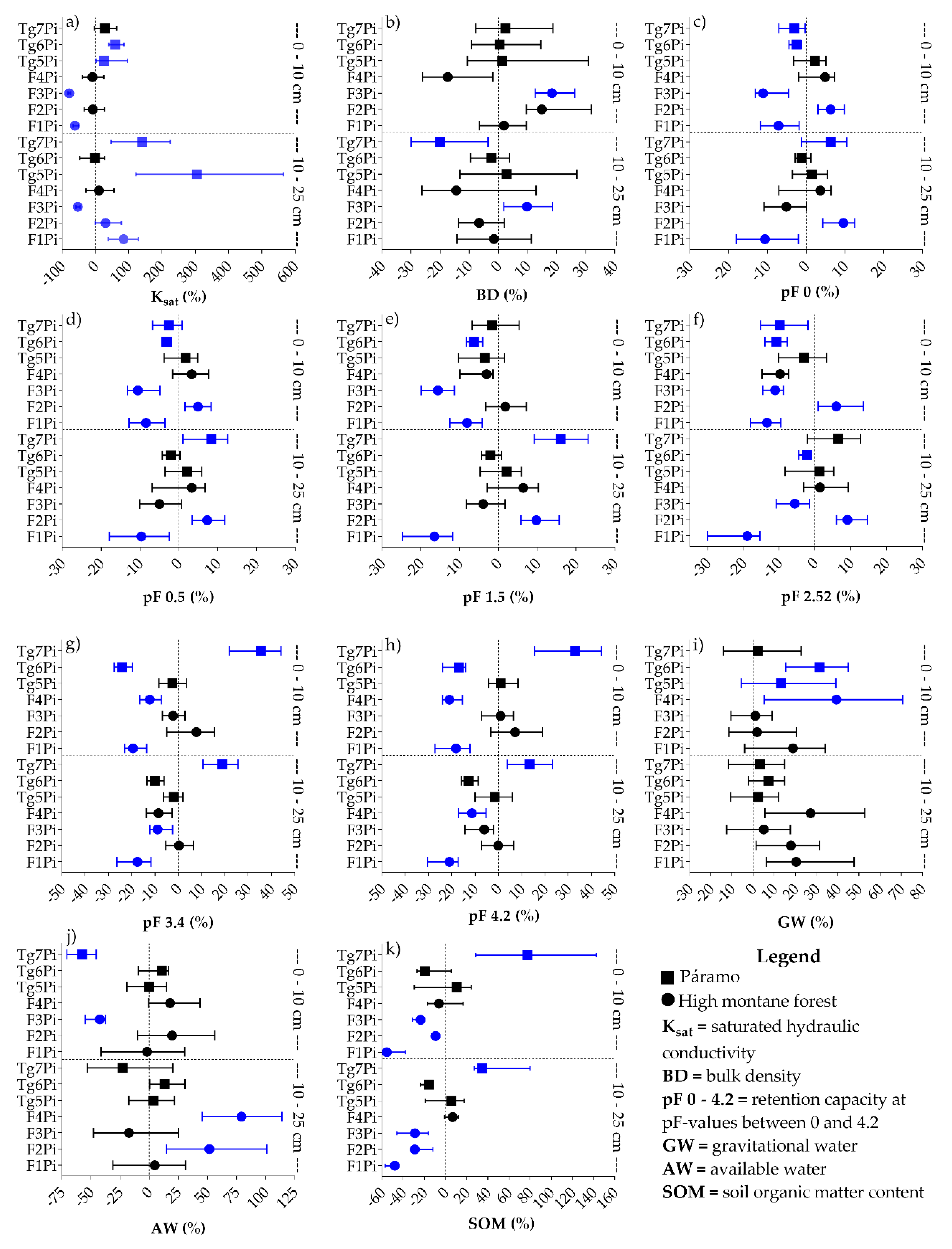
3.3. Changes in Hydro-Physical and SOM Content under Pine Afforestation

The properties found at each of the pine afforested and grazing sites in the 0–10 and 10–25 cm soil layers are presented in the Appendix, in Table A2 (pine plantation) and Table A3 (grazing). According to the Mann-Whitney U test (p < 0.05), the properties in the pine plantations in the 0–10 cm layer were significantly different from the characteristics measured in the 10–25 cm soil layer. Therefore, the impacts of pine afforestation were evaluated considering both depths. On the other hand, there were no significant differences (p > 0.05) in the properties between sampling distances (75 and 150 cm) from the trees in each of the pine plantations (

Table A4. p-values of the comparisons of the hydro-physical properties between 75 and 150 cm of sampling distance in each of the pine plantations in the study area. Elevation: <3250 m a.s.l., >3250–<3550 m a.s.l., >3550 m a.s.l.

	Elevation	<3250 m a.s.l.		>3250–<3550 m a.s.l.			>3550 m a.s.l.
	Properties	F1Pi	F2Pi	F3Pi	F4Pi	Tg5Pi	Tg6Pi	Tg7Pi
0–10 cm soil layer	Ksat	0.16	0.59	0.19	0.18	0.36	0.45	0.66
	BD	0.62	0.82	0.92	0.76	0.92	0.79	0.91
	0 pF	0.48	0.4	0.38	0.74	0.76	0.3	0.93
	0.5 pF	0.97	0.43	0.59	0.9	0.76	0.53	0.94
	1.5 pF	0.97	0.8	0.71	0.08	0.77	0.55	0.93
	2.52 pF	0.65	0.95	0.36	0.24	0.97	0.42	0.79
	3.4 pF	0.18	0.53	0.27	0.25	0.24	0.88	0.45
	4.2 pF	0.32	0.74	0.42	0.19	0.18	0.37	0.93
	GW	0.93	0.43	0.48	0.32	0.68	0.77	0.58
	AW	0.8	0.71	0.2	0.81	0.52	0.59	1
10–25cm soil layer	Ksat	0.56	0.9	0.03	0.38	0.54	0.82	0.21
	BD	0.97	0.76	0.97	0.93	0.97	0.84	0.91
	0 pF	0.98	0.74	0.6	1	0.97	0.76	0.89
	0.5 pF	0.92	0.66	0.51	0.92	0.9	0.82	0.84
	1.5 pF	0.9	0.58	0.74	0.88	0.92	0.95	0.78
	2.52 pF	0.66	0.34	0.68	0.79	0.8	0.87	0.94
	3.4 pF	0.88	0.03	0.19	0.69	0.68	0.77	1
	4.2 pF	0.6	0.14	0.93	0.25	0.76	0.12	0.58
	GW	0.66	0.53	0.3	0.9	0.79	0.79	0.91
	AW	0.51	0.19	0.49	0.2	0.87	0.12	0.67

The names of the variables are defined in Table 4. The values in bold indicate that the properties are significantly different between both depths (p < 0.05).

), suggesting that sampling could have been carried out at either of these distances. Therefore, the properties’ values measured at a distance of 75 and 150 cm from the tree trunk were grouped by depth.

Pine afforestation produced significant changes in the hydro-physical properties and SOM content in both layers as depicted in the forest plots of Figure 2 and Appendix Table A2. K_sat of the upper layer decreased significantly in the F1Pi and F3Pi plantations (61.72% and 79.06%, respectively), which are located in the high montane forest area. In the páramo plantations, the K_sat value increased significantly in two of the three plantations (Tg5Pi and Tg6Pi) by 25.23 and 59.22%, respectively (see Figure 2a). The BD value did not show significant changes in most of the sites except for F3Pi which increased significantly by 18.42% (Figure 2b). As further depicted in Figure 2c, the water retention capacity at saturation (pF 0) in the upper layer decreased significantly in the F1Pi, F3Pi, Tg6Pi and Tg7Pi sites, with a reduction between 2.53% and 11.10%, while in F2Pi the water content at saturation increased significantly by 6.30% (Figure 2c). The changing tendency in water retention capacity in the pF range from 0.5 to 2.52 (see Figure 2d–f) was similar to the change in the water retention capacity at pF 0 in most of the plantations, supporting the conclusion that pine afforestation led to significant changes in the soil’s hydro-physical properties. The water retention capacity at pF 3.4 and pF 4.2 (Figure 2g,h) decreased meaningfully between 12.21% and 27.52% in the F1Pi, F4Pi, and Tg6Pi sites, but differently in the Tg7Pi site where the increase was significant, varying between 15.54% and 44.31%. The GW in F4Pi, Tg5Pi and Tg6Pi increased significantly (13.15%–39.37%) (Figure 2i), while AW decreased considerably in F3Pi and Tg7Pi, with a reduction varying between 42.50% and 57.64%, (Figure 2j). The SOM content in F1Pi, F2Pi and F3Pi decreased considerably, by 28.97%, 29.00% and 47.90% (Figure 2k); while in Tg7Pi the SOM content was significantly reduced by 77.62%.

The K_sat increased significantly in the 10–25 cm layer in the F1Pi, F2Pi, Tg5Pi and Tg6Pi sites by 84.64%, 30.28%, 305.24% and 140%, respectively; while in F3Pi the K_sat was significantly reduced by 52.98% (Figure 2a). There was a significant increase of BD in F3Pi (9.81%), in contrast to Tg7Pi where there was a significant reduction of 2.47% (Figure 2b). Regarding the water retention capacity at saturation, F1Pi declined significantly by 10.62%, contrasting with F2Pi and Tg7Pi where there was a significant increment by 9.60% and 6.32%, respectively (Figure 2c). Similar results were obtained for water retention capacity in pF 0.5 to pF 1.5 (Figure 2d,e). Water retention at field capacity decreased significantly in F1Pi, F3Pi and Tg6Pi by 18.92%, 5.68% and 2.2%, respectively, whereas it increased significantly at F2Pi by 9.06% (Figure 2f). The retention capacities at pFs 3.4 and 4.2 decreased significantly between 2.62% and 30.35% at sites F1Pi and F4Pi (Figure 2g,h); whereas they increased significantly between 3.90 and 25.56% at site Tg7Pi. The GW did not show significant changes in any of the plantations. AW in the F2Pi and F4Pi plantations presented a significant increase of 51.55% and 79%. The SOM content in F1Pi, F2Pi and F3Pi decreased considerably by 55.50%, 9.32% and 23.50%, respectively, differently from Tg7Pi where there was a significant increase by 77.62% (Figure 2k).

Correlation analysis revealed that K_sat in the 0–10 cm and 10–25 cm layers presents strong correlations with tree development variables DBH, Ht and CD, and there is clearly an increase of K_sat with increasing tree height (data not shown). Likewise, the BD in both layers was also positively correlated with the tree development variables (ρ ≥ 0.31, p < 0.05). That is to say, with an increase in tree growth, there is a significant increment in soil BD. On the other hand, water retention capacity and SOM contents are negatively correlated with tree development variables (ρ ≥ 0.31, p < 0.05). That is, in both soil layers (0–10 and 10–25 cm), water retention capacity and SOM content decrease significantly with tree development.

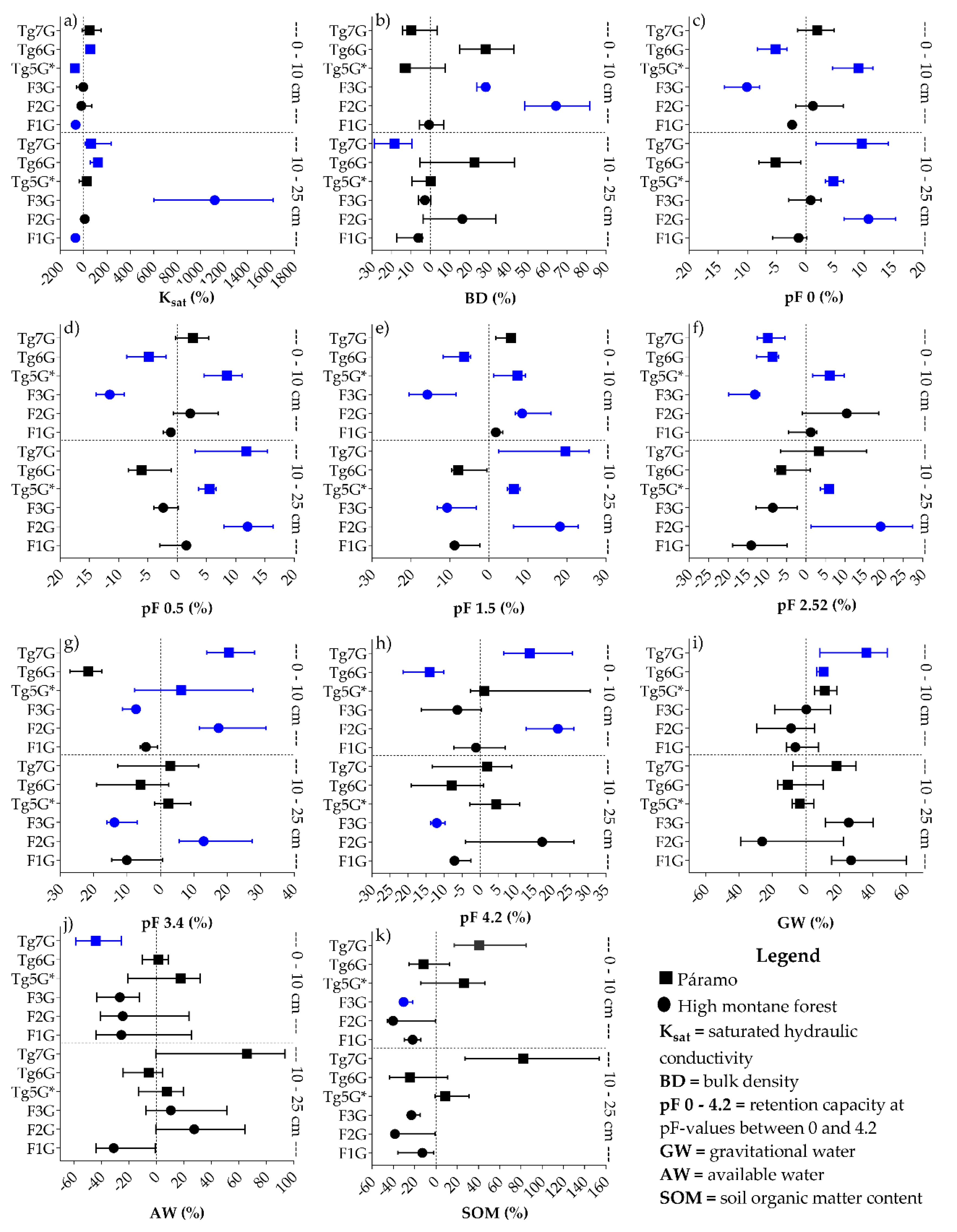
3.4. Changes in Hydro-Physical and SOM Content under Grazing

The Mann-Whitney U test (p < 0.05) revealed significant changes in the soil’s hydro-physical properties under grazing, which was reflected mainly in the K_sat and water retention capacity (Appendix: Table A3). There were a higher number of sites with significant changes in the studied soil hydro-physical properties in the 0–10 cm surface layer, than in the 10–25 cm soil layer (Figure 3). In the upper layer, K_sat decreased significantly in the F1G and Tg5G * sites by 68.87% and 75.75%, respectively, while there was a significant increase of 55.19% in Tg6G (Figure 3a). With respect to the BD in F2G and F3G, there was a significant increase of 64.29% and 28.25% (Figure 3b). The water retention capacity at saturation in F3G and Tg6G decreased significantly by 10.10% and 5.18%, respectively, while it increased significantly by 8.97% in Tg5G * (Figure 3c). The changes in water retention capacity at pF 0.5 and pF 1.5 were similar to those at pF 0 (Figure 3d,e). Water retention capacity at pF 2.52 decreased significantly in the F3G, Tg6G and Tg7G sites by 13.11%, 8.61% and 9.77%, respectively. On the other hand, there was a significant increment of 10.46% at F2G (Figure 3f). The water retention capacity at pF 3.4 increased significantly at the sites F2G, Tg5G * and Tg7G by 17.38%, 6.15% and 20.46%, respectively. Conversely, the water retention at field capacity decreased by 7.36% in F3G. The changes in water retention at wilting point (pF 4.2) were similar to those at pF 3.4 (Figure 3g,h) at the sites with significant changes, except for F3G. Changes in GW (Figure 3i) were noticed in the Tg6G and Tg7G sites, with an increase of 10.59% and 36.12%, respectively. The AW (Figure 3j) and the SOM content (Figure 3k) did not show significant changes in the majority of the study sites, except the for SOM content in site F3G where there was a significant reduction of 30.47%.

In the soil layer 10–25 cm, K_sat decreased significantly by 71.01% in the F1G site, by 1120.09% in F3G, by 121.28% in Tg6G, and by 61.35% in the Tg7G site (Figure 3a). The BD did not show significant changes in the grazing sites, except for Tg7G where it decreased significantly by 18.63% (Figure 3b). The water retention capacity at pF 0 increased significantly by 10.71%, 4.67% and 9.57% in the F2G, Tg5G * and Tg7G sites (Figure 3c). At these sites, the trends followed by the changes in water retention capacity at pF 0.5 and pF 1.5 were similar to those at pF 0 (Figure 3d,e). At pF 2.52, the water retention capacity at F2G and Tg5G * increased significantly by 19.17% and 5.92%, respectively (Figure 3f). The water retention capacity at pF 3.4 increased significantly by 12.92% at site F2G, unlike F3G where a significant reduction of 13.78% was found (Figure 3g). Most sites did not display significant changes in the water retention capacity at wilting point, except for F3G, where there was a significant reduction of 12.06% (Figure 3h). Finally, GW, AW, and the SOM content did not show significant changes at all study sites (Figure 3i–k).

4. Discussion

Some studies in sites close to the study presented herein evaluated the impacts of anthropogenic activities by grouping soils by their conditions of natural undisturbed land cover, without considering their elevation and sampling depth [19,28,29]. In our study, results suggest that in order to evaluate the impacts of any anthropogenic activity, it is essential to examine the spatial variability of soils under natural conditions or at least to avoid evaluating the impacts based on sampling sites located in different places. In other words, the impacts of anthropogenic activities on soils should be done in adjacent sites, which would guarantee similar geomorphological and climatic conditions [58]. Even the spatial variability of soils is often the cause that the hydrological performance of Andean ecosystems can be extremely heterogeneous [26,59]. That is, the high variability of soils under natural conditions can even cause variability in the functioning of basins.

An aspect often discussed in monitoring the impact of afforestation on soils is at what distance from the trunk and what depth should samples preferably be collected. A previous study in Andean highlands suggested that changes in soil properties in pine plantations differ depending on the sampling distance from the trunk of the tree [15]. However, in all the plantations within our study area, the hydro-physical properties did not differ between the tested sampling distances of 75 and 150 cm away from the trunk. These results are consistent with what Wilcox, Breshears & Turin [60] and Ruiz et al. [61] reported. Wilcox et al. [60] stated that the K_sat of the soil under the canopy and between the canopy of the pine trees did not show significant differences. Likewise, Ruiz et al. [61] reported that the water retention capacity and AW in the soil did not differ between 50 cm from the base of the trunk vs. under the crown of the tree. On the other hand, according to our results, the hydro-physical properties and the SOM content showed significant differences between the two sampling depths (0–10 cm and 10–25 cm) in each of the plantations, a finding in line with the results of Ghimire et al. [62]. Our results suggest that pine afforestation effectively impacts in a different way the soil properties as a function of depth, but not as a function of the distance samples are collected from the tree trunk.

The comparisons of the properties of each plantation with their respective adjacent natural cover revealed that the intervention of the soils through, for example, pine afforestation in the Andean ecosystems mainly affects K_sat, water retention capacity between saturation (pF 0) and field capacity (pF 2.52), and SOM content, and this at both sampling depths but at a different intensity. Due to these changes, pine plantations could directly alter the ecosystem services such as water regulation and storage [25,26] and the carbon sequestration by soils [63]. However, findings could not be generalized, showing dependencies mainly in the sampling depth, ecosystem type, characteristics of the plantations, and previous land-use. This implies a complexity in assessing the impacts of plantations and limits the generalization capability of changes in soil properties caused by pine plantations in high Andean ecosystems.

According to Alarcón et al. [64], changes due to grazing were not statistically evident in the K_sat measured in the 0–10 cm soil layer in Andosols. However, our results partially contradict this because 2 (F1G and Tg5G *) of the 6 study sites showed a significant reduction in K_sat up to 70%, while in the Tg6G site a significant increase of 52.67% was registered. The reduction in K_sat at the F1G site could be due to the loss of stability of the soil aggregates and grazing density, while the reduction in K_sat at Tg5G * is likely the consequence of the frequent burning of tussock grass resulting in a drying and crusting of the soil surface [65]. On the other hand, although the increase in K_sat was not significant at Tg7G, this percentage increase was very similar to that at the Tg6G site (Figure 3a). The increase at both these sites is likely related to preferential flows between the clods formed by soil tillage [66] during the preparation and sowing of pasture. However, this situation could apparently change over time due to the structural deterioration of the soil.

Despite the lack of significant evidence, it was observed that in 6 of the 7 pine plantations, BD tended to increase in the 0–10 cm soil layer, which certainly cannot be the consequence of the use of heavy machinery for maintenance since the associated high costs and the difficult topographic conditions prevent the use of machines [67]. Rather the drying of the soil by evapotranspiration [68] and the weight of the trees [69] are responsible for the increase in BD, which is confirmed in our study by a greater increase in BD in the sites where the pine plantation is characterized by high SD and CD (e.g., F2Pi and F3Pi in high montane forest and Tg5Pi in páramo). The BD at 10–25 cm depth was not affected in most of the plantations; however, most plantations showed a decreasing trend ranging from 2% to 18%. This tendency is attributable to the increase of porosity generated by the pine subsurface root system. On the other hand, two plantations (F3Pi and Tg5Pi) showed an increase which is attributable to the compaction by the pressure exerted by the biomass of the plantation on the soil, due to its high SD, which translates into a greater number of trees, increasing the transpiration, and resulting in soil contraction.

The compaction of the soil by grazing is normally directly reflected in an increase of the BD [70,71]. However, this effect was only observed in two study sites (F2G and F3G) and the direct consequence of the greater grazing intensity at these sites (ABU Ha⁻¹ of 2 and 1, respectively), parallel to a decomposition of SOM. Our findings are consistent with those of Donkor et al. [72] where an increase in compaction was directly related to a greater grazing intensity. In páramo, the trampling effect of cattle was not reflected in the measurements, which was consistent with the results of Alarcón et al. [64] and Podwojewski et al. [23]. Their results and our study suggest that Andosols (due to their high SOM content) have a greater resilience to compaction [73] given the overall low-grazing intensity (ABU Ha⁻¹ of <0.5). Because of the lack of significant evidence, our results do not permit to conclude that grazing significantly compacted the soil at the 10–25 cm depth. This may be due to the high SOM content of the Andosols. In the case of Tg7G, where BD decreased significantly by 18.63%, this decrease is likely caused by the incorporation of tussock grass biomass during tillage.

Pine plantations alter the water retention capacity of soils according to Farley et al. [20]. This is confirmed by the results of this study, with the difference that the alteration is not only dependent on associated changes in the SOM content, but also on elevation, ecosystem type, the development level of the plantation and land-use, as reported in other ecosystems [56,63,74]. The highest reduction percentages in our study were attributed to a greater development of the plantations (DBH >18 cm, Ht >8 m and CD >5 m), together with a decrease in SOM and increase in BD. In the three plantations that were established on soils whose previous use was grazing (F4Pi, Tg5Pi and Tg7Pi), the changes in water retention capacity were very variable, observing significant increases or decreases between pF 0 and pF 2.52, notwithstanding the SOM content tended to increase. This variation in the changes could be due to a mixture of changes between the previous use of the soil and the growth of the plantation [61,74]. This apparent overlap of impacts [62] hinders generalization of changes. On the other hand, our data show an increase in water retention is not necessarily always related to an increase in SOM content, but can also be the consequence of an increase in clay content due to the weathering of the soil [75,76]. In general, pine afforestation goes hand in hand with an increase in GW and a decrease in AW, suggesting that soils under pine plantations rapidly lose moisture after a rainfall event, which further enhances soil drying and decomposition of SOM [77]. On the other hand, according to Buytaert et al. [22], land use change could increase the AW of soils of volcanic origin by 30%. On the contrary, Hofstede et al. [19] reported a decrease in AW as a consequence of pine afforestation. Nevertheless, in our study, only two pine plantations showed a significant decrease (F3Pi and Tg7Pi).

Under grazing, it has been shown that the loss of water retention is mainly a result of a reduction in SOM content. Increases in water retention capacity were explicitly related to increases in SOM content due to burning and/or the incorporation of tussock grass during soil preparation. This finding is in line with Daza et al. [32] who reported that in their study the decrease in soil water retention was due to a loss of SOM content. However, in the F2G site the increase of the water retention capacity was the result of the easy weathering of volcanic glass, leading to the formation of montmorillonite clay [76]. The latter indicates that in order to correctly assess changes in, for example, the hydro-physical properties in soils, it is essential to evaluate the full spectrum of soil properties such as SOM, soil texture, type of management, among others.

Notwithstanding that several studies associate the reduction of SOM content with pine afforestation [19,20,58], our findings indicate that pine plantations could help the recovery of SOM in the 0–10 cm soil layer of former grazing sites, though the effect seems also to depend on the elevation of the site and the SD of the plantation. Although the SOM content did not show significant changes under grazing, a reduction in most of the study sites was detected. This slightly decreasing trend would imply that, over time, the soils under grazing in the Andean region could lose a considerable amount of SOM, and thus, reduce their capacity to retain water.

5. Conclusions

Andosols with their black Andic horizon are the predominant soils in Andean montane ecosystems. Our research clearly revealed that this horizon, with high water retention capacity and SOM content, is not that uniform under natural unaltered conditions. Differences in hydro-physical properties, such as K_sat and the water retention capacity, are related to the type of ecosystem and elevation of the terrain. Differences in properties not only occur between sites, but also within sites at different depths of sampling. As a result, higher values of K_sat, water retention capacity and SOM content were recorded in the 0–10 cm surface layer. The natural spatial variability in environmental conditions and the accompanied heterogeneity in soil properties requires that for the correct assessment of the impact of land use change, data are collected on neighboring comparable, unaltered and altered sites. Doing so will facilitate and help guarantee that a correct assessment of the causal factors that positively or negatively affect the soil hydro-physical properties by land use change, is drawn. Furthermore, the multitude of observations and their analyses clearly revealed that the impact of land-use change on the hydro-physical soil properties is not unique and often masked by other factors such as the antecedent land-use, spatial variability, pre-tilling and tilling activities, soil texture, elevation, climate, among other site-specific factors. Due to these differences, it is rather difficult to evaluate the impacts of pine plantations and grazing on properties at regional scale, and therefore any evaluation of the impacts of anthropogenic activities must be carried out in adjacent sites, which would guarantee similar geomorphological and climatic conditions. This conclusion clearly points out that generalization of findings related to the impacts of land use change on soil properties is not free of risks. Similarly, it also hinders the comparison of findings with published results.

The study further revealed that pine afforestation affects either in a positive or negative way the K_sat, the water retention capacity in the range pF 0 to 2.52 and the SOM content of the soil surface layer. The change and the order of magnitude of the change varies with sampling depth. Similarly, grazing causes positive and negative changes in K_sat and in the water retention capacity, and as in pine plantations, the recorded changes vary with sampling depth. Other controlling factors that define the impact of grazing are evidently pre-tilling and tilling activities in combination with cattle density. Soil spatial heterogeneity and diversity in local factors complicates the interpretation and extrapolation of observed phenomena to Andean montane ecosystems at a regional scale. Correct assessment of land use change impacts is not only of crucial importance for extrapolating findings, it also serves as a basis for the accurate estimation of socio-economic and ecological impacts that anthropogenic-induced changes might have on the water regulation and water storage functionalities of the Andic soils.

References

1. Buytaert, W.; Cuesta-Camacho, F.; Tobón, C. Potential impacts of climate change on the environmental services of humid tropical alpine regions. Glob. Ecol. Biogeogr. 2011, 20, 19–33. [Google Scholar] [CrossRef]
2. Célleri, R.; Feyen, J. The hydrology of tropical Andean ecosystems: Importance, knowledge status, and perspectives. Mt. Res. Dev. 2009, 29, 350–355. [Google Scholar] [CrossRef]
3. Mosquera, G.; Lazo, P.; Célleri, R.; Wilcox, B.; Crespo, P. Runoff from tropical alpine grasslands increases with areal extent of wetlands. Catena 2015, 125, 120–128. [Google Scholar] [CrossRef] [Green Version]
4. Mosquera, G.; Célleri, R.; Lazo, P.; Vaché, K.; Perakis, S.; Crespo, P. Combined use of isotopic and hydrometric data to conceptualize ecohydrological processes in a high-elevation tropical ecosystem. Hydrol. Process. 2016, 30, 2930–2947. [Google Scholar] [CrossRef] [Green Version]
5. Correa, A.; Windhorst, D.; Tetzlaff, D.; Crespo, P.; Célleri, R.; Feyen, J.; Breuer, L. Temporal dynamics in dominant runoff sources and flow paths in the Andean Páramo. Water Resour. Res. 2017, 53, 5998–6017. [Google Scholar] [CrossRef] [Green Version]
6. Buytaert, W.; Celleri, R.; Willems, P.; De Bievre, B.; Wyseure, G. Spatial and temporal rainfall variability in mountainous areas: A case study from the south Ecuadorian Andes. J. Hydrol. 2006, 329, 413–421. [Google Scholar] [CrossRef] [Green Version]
7. Poulenard, J.; Podwojewski, P.; Herbillon, A.J. Characteristics of non-allophanic Andisols with hydric properties from the Ecuadorian páramos. Geoderma 2003, 117, 267–281. [Google Scholar] [CrossRef]
8. Hofstede, R.; Lips, J.; Jongsma, W. Geografía, Ecología y Forestación de la Sierra Alta del Ecuador; Abya-Yala: Quito, Ecuador, 1998; ISBN 9978044213. [Google Scholar]
9. Mena, P.; Josse, C.; Medina, G. Los Suelos del Páramo; GTP/Abya-Yala: Quito, Ecuador, 2000. [Google Scholar]
10. Buytaert, W.; Deckers, J.; Dercon, G.; De Bièvre, B.; Poesen, J.; Govers, G. Impact of land use changes on the hydrological properties of volcanic ash soils in South Ecuador. Soil Use Manag. 2002, 18, 94–100. [Google Scholar] [CrossRef]
11. Shoji, S.; Nanzyo, M.; Dahlgren, R. Volcanic Ash Soils: Genesis, Properties and Utilization; Elsevier: Amsterdam, The Netherlands, 1993. [Google Scholar]
12. Buytaert, W.; Célleri, R.; De Bièvre, B.; Cisneros, F.; Wyseure, G.; Deckers, J.; Hofstede, R. Human impact on the hydrology of the Andean páramos. Earth-Sci. Rev. 2006, 79, 53–72. [Google Scholar] [CrossRef] [Green Version]
13. Mena, P.; Hofstede, R. Los páramos ecuatorianos. Bot. Econ. Los Andes Cent. 2006, 91–109. [Google Scholar]
14. Buytaert, W.; Iñiguez, V.; De Bièvre, B. The effects of afforestation and cultivation on water yield in the Andean páramo. For. Ecol. Manag. 2007, 251, 22–30. [Google Scholar] [CrossRef] [Green Version]
15. Harden, C.P.; Hartsig, J.; Farley, K.A.; Lee, J.; Bremer, L.L. Effects of land-use change on water in Andean páramo grassland soils. Ann. Assoc. Am. Geogr. 2013, 103, 375–384. [Google Scholar] [CrossRef]
16. Knoke, T.; Bendix, J.; Pohle, P.; Hamer, U.; Hildebrandt, P.; Roos, K.; Gerique, A.; Sandoval, M.L.; Breuer, L.; Tischer, A.; et al. Afforestation or intense pasturing improve the ecological and economic value of abandoned tropical farmlands. Nat. Commun. 2014, 5, 5612. [Google Scholar] [CrossRef] [PubMed] [Green Version]
17. Farley, K.A.; Kelly, E.F. Effects of afforestation of a páramo grassland on soil nutrient status. For. Ecol. Manag. 2004, 195, 271–290. [Google Scholar] [CrossRef]
18. Hofstede, R. El Impacto de las Actividades Humanas sobre el Páramo; Abya-Yala: Quito, Ecuador, 2001. [Google Scholar]
19. Hofstede, R.G.M.; Groenendijk, J.P.; Coppus, R.; Fehse, J.C.; Sevink, J. Impact of pine plantations on soils and vegetation in the Ecuadorian high Andes. Mt. Res. Dev. 2002, 22, 159–167. [Google Scholar] [CrossRef]
20. Farley, K.A.; Kelly, E.F.; Hofstede, R.G.M. Soil organic carbon and water retention after conversion of grasslands to pine plantations in the Ecuadorian Andes. Ecosystems 2004, 7, 729–739. [Google Scholar] [CrossRef]
21. Medina, G.; Josse, C.; Mena, A. La forestación en los páramos. Ser. Páramo 2000, 6, 1–76. [Google Scholar]
22. Buytaert, W.; Wyseure, G.; De Bièvre, B.; Deckers, J. The effect of land-use changes on the hydrological behaviour of Histic Andosols in south Ecuador. Hydrol. Process. 2005, 19, 3985–3997. [Google Scholar] [CrossRef] [Green Version]
23. Podwojewski, P.; Poulenard, J.; Zambrana, T.; Hofstede, R. Overgrazing effects on vegetation cover and properties of volcanic ash soil in the páramo of Llangahua and La Esperanza (Tungurahua, Ecuador). Soil Use Manag. 2002, 18, 45–55. [Google Scholar] [CrossRef]
24. López, M.; Veldkamp, E.; de Koning, G.H.J. Soil carbon stabilization in converted tropical pastures and forests depends on soil type. Soil Sci. Soc. Am. J. 2005, 69, 1110–1117. [Google Scholar] [CrossRef]
25. Ochoa, B.F.; Buytaert, W.; De Bièvre, B.; Célleri, R.; Crespo, P.; Villacís, M.; Llerena, C.A.; Acosta, L.; Villazón, M.; Guallpa, M.; et al. Impacts of land use on the hydrological response of tropical Andean catchments. Hydrol. Process. 2016, 30, 4074–4089. [Google Scholar] [CrossRef] [Green Version]
26. Crespo, P.J.; Feyen, J.; Buytaert, W.; Bücker, A.; Breuer, L.; Frede, H.-G.; Ramírez, M. Identifying controls of the rainfall–runoff response of small catchments in the tropical Andes (Ecuador). J. Hydrol. 2011, 407, 164–174. [Google Scholar] [CrossRef]
27. Greenwood, W.J.; Buttle, J.M. Effects of reforestation on near-surface saturated hydraulic conductivity in a managed forest landscape, southern Ontario, Canada. Ecohydrology 2012, 7, 45–55. [Google Scholar] [CrossRef]
28. Quichimbo, P.; Tenorio, G.; Borja, P.; Cardenas, I.; Crespo, P.; Celleri, R. Efectos sobre las propiedades físicas y químicas de los suelos por el cambio de la cobertura vegetal y uso del suelo: Páramo de Quimsacocha al sur del Ecuador. Suelos Ecuat. 2012, 42, 138–153. [Google Scholar]
29. Chacón, G.; Gagnon, D.; Paré, D. Comparison of soil properties of native forests, Pinus patula plantations and adjacent pastures in the Andean highlands of southern Ecuador: Land use history or recent vegetation effects? Soil Use Manag. 2009, 25, 427–433. [Google Scholar] [CrossRef]
30. La Manna, L.; Buduba, C.G.; Rostagno, C.M. Soil erodibility and quality of volcanic soils as affected by pine plantations in degraded rangelands of NW Patagonia. Eur. J. For. Res. 2016, 135, 643–655. [Google Scholar] [CrossRef]
31. De Koning, G.H.J.; Veldkamp, E.; López-Ulloa, M. Quantification of carbon sequestration in soils following pasture to forest conversion in northwestern Ecuador. Glob. Biogeochem. Cycles 2003. [Google Scholar] [CrossRef]
32. Daza, M.C.; Hernández, F.; Triana, F.A. Efecto del uso del suelo en la capacidad de almacenamiento hídrico en el páramo de Sumapaz-Colombia. Rev. Fac. Nac. Agron. Medellín 2014, 67, 7189–7200. [Google Scholar] [CrossRef]
33. Celik, I. Land-use effects on organic matter and physical properties of soil in a southern Mediterranean highland of Turkey. Soil Tillage Res. 2005, 83, 270–277. [Google Scholar] [CrossRef]
34. Buytaert, W.; Deckers, J.; Wyseure, G. Regional variability of volcanic ash soils in south Ecuador: The relation with parent material, climate and land use. Catena 2007, 70, 143–154. [Google Scholar] [CrossRef]
35. Bussmann, R. Bosques andinos del sur del Ecuador, classificación, regeneración y uso. Rev. Peru. Biol. 2005, 12, 203–216. [Google Scholar]
36. Baquero, F.; Sierra, R.; Ordóñez, L.; Tipán, M.; Espinoza, L.; Rivera, M.; Soria, P. La Vegetación de los Andes del Ecuador: Memoria explicativa de los mapas de vegetación potencial y remanente de los Andes del Ecuador a escala 1:250.000 y del modelamiento predictivo con especies indicadoras; EcoCiencia: Quito, Ecuador, 2004; ISBN 9978439994. [Google Scholar]
37. Ramsay, P.; Oxley, E. The growth form composition of plant communities in the Ecuadorian páramos. Plant Ecol. 1997, 131, 173–192. [Google Scholar] [CrossRef]
38. Luteyn, J.L. Páramos: A Checklist of Plant Diversity, Geographical Distribution, and Botanical Literature; The New York Botanical Garden Press: New York, NY, USA, 1999. [Google Scholar]
39. Vuille, M.; Bradley, R.; Keimig, F. Climate variability in the Andes of Ecuador and its relation to tropical Pacific and Atlantic sea surface temperature anomalies. J. Clim. 2000, 13, 2520–2535. [Google Scholar] [CrossRef]
40. Córdova, M.; Célleri, R.; Shellito, C.J.; Orellana-Alvear, J.; Abril, A.; Carrillo-Rojas, G. Near-surface air temperature lapse rate over complex terrain in the southern Ecuadorian Andes: Implications for temperature mapping. Arct. Antarct. Alp. Res. 2016, 48, 673–684. [Google Scholar] [CrossRef]
41. Padrón, R.S.; Wilcox, B.P.; Crespo, P.; Célleri, R. Rainfall in the Andean páramo: New insights from high-resolution monitoring in southern Ecuador. J. Hydrometeorol. 2015, 16, 985–996. [Google Scholar] [CrossRef]
42. Hungerbühler, D.; Steinmann, M.; Winkler, W.; Seward, D.; Egüez, A.; Peterson, D.; Helg, U.; Hammer, C. Neogene stratigraphy and Andean geodynamics of southern Ecuador. Earth-Sci. Rev. 2002, 57, 75–124. [Google Scholar] [CrossRef]
43. IUSS Working Group WRB. World Reference Base for Soil Resources 2014, Update 2015 International Soil Classification System for Naming Soils and Creating Legends for Soil Maps; FAO: Rome, Italy, 2015. [Google Scholar]
44. Buytaert, W.; Sevink, J.; De Leeuw, B.; Deckers, J. Clay mineralogy of the soils in the south Ecuadorian páramo region. Geoderma 2005, 127, 114–129. [Google Scholar] [CrossRef] [Green Version]
45. Aucapiña, G.; Marín, F. Efectos de la Posición Fisiográfica en las Propiedades Hidrofísicas de los Suelos de Páramo de la Microcuenca del río Zhurucay; Universidad de Cuenca: Cuenca, Ecuador, 2014. [Google Scholar]
46. Quiroz, C.; Crespo, P.; Stimm, B.; Murtinho, F.; Weber, M.; Hildebrandt, P. Contrasting stakeholders’ perceptions of pine plantations in the páramo ecosystem of Ecuador. Sustainability 2018, 10, 1707. [Google Scholar] [CrossRef]
47. Food and Agriculture Organization of the United Nations. Guidelines for Soil Description, 4th ed.; Jahn, R., Blume, H., Asio, V., Spaargaren, O., Schad, P., Eds.; FAO: Rome, Italy, 2006. [Google Scholar]
48. Oosterbaan, R.; Nijland, H. Determining the saturated hydraulic conductivity. In Drainage Principles and Applications; International Institute for Land Reclamation and Improvement: Wageningen, The Netherlands, 1994; pp. 1–38. ISBN 90 70754 3 39. [Google Scholar]
49. Food and Agriculture Organization of the United Nations. Procedures for Soil Analysis, 6th ed.; van Reeuwijk, L.P., Ed.; FAO: Roma, Italy, 2002. [Google Scholar]
50. Guo, L.; Gifford, M. Soil carbon stocks and land use change: A meta analysis. Glob. Chang. Biol. 2002, 8, 345–360. [Google Scholar] [CrossRef]
51. Topp, G.C.; Zebchuk, W. The determination of soil-water desorption curves for soil cores. Can. J. Soil Sci. 1979, 59, 19–26. [Google Scholar] [CrossRef]
52. Kruskal, W.; Wallis, W. Use of ranks in one-criterion variance analysis. J. Am. Stat. Assoc. 1952, 47, 583–621. [Google Scholar] [CrossRef]
53. Nemenyi, P. Distribution-free multiple comparisons. Biometrics 1962, 18, 263. [Google Scholar]
54. Mann, H.B.; Whitney, D.R. On a test of whether one of two random variables is stochastically larger than the other. Ann. Math. Stat. 1947, 18, 50–60. [Google Scholar] [CrossRef]
55. Sakia, R.M. The Box-Cox transformation technique: A review. J. R. Stat. Soc. Ser. D 1992, 41, 169–178. [Google Scholar] [CrossRef]
56. Martín, F.; Navarro, F.; Jiménez, M.; Sierra, M.; Martínez, F.; Romero, A.; Rojo, L.; Fernández, E. Long-term effects of pine plantations on soil quality in southern Spain. L. Degrad. Dev. 2016. [Google Scholar] [CrossRef]
57. R Development Core Team. R: A Language and Environment for Statistical Computing; R Foundation for Statistical Computing: Vienna, Austria, 2016. [Google Scholar]
58. Broquen, P.; Girardin, J.; Frugoni, M. Evaluación de algunas propiedades de suelos derivados de cenizas volcánicas asociadas con forestaciones de coníferas exóticas (S.O. de la provincia de Neuquén-R. Argentina). Bosque 1995, 16, 69–79. [Google Scholar] [CrossRef]
59. Suárez, E.; Arcos, E.; Moreno, C.; Encalada, A.; Álvarez, M. Influence of vegetation types and ground cover on soil water infiltration capacity in a high-altitude páramo ecosystem. Av. Cienc. Ing. 2013, 5, B14–B21. [Google Scholar]
60. Wilcox, B.P.; Breshears, D.D.; Turin, H.J. Hydraulic conductivity in a Pinon-Juniper woodland: Influence of vegetation. Soil Sci. Soc. Am. J. 2003, 67, 1243–1249. [Google Scholar] [CrossRef]
61. Ruiz, A.; Barberá, G.G.; Navarro, J.A.; Albaladejo, J.; Castillo, V.M. Soil dynamics in Pinus halepensis reforestation: Effect of microenvironments and previous land use. Geoderma 2009, 153, 353–361. [Google Scholar] [CrossRef]
62. Ghimire, C.P.; Bonell, M.; Bruijnzeel, L.A.; Coles, N.A.; Lubczynski, M.W. Reforesting severely degraded grassland in the Lesser Himalaya of Nepal: Effects on soil hydraulic conductivity and overland flow production. J. Geophys. Res. Earth Surf. 2013, 118, 2528–2545. [Google Scholar] [CrossRef] [Green Version]
63. Liao, C.; Luo, Y.; Fang, C.; Chen, J.; Li, B. The effects of plantation practice on soil properties based on the comparison between natural and planted forests: A meta-analysis. Glob. Ecol. Biogeogr. 2012, 21, 318–327. [Google Scholar] [CrossRef]
64. Alarcón, C.; Dörner, J.; Dec, D.; Balocchi, O.; López, I. Efecto de dos intensidades de pastoreo sobre las propiedades hidráulicas de un andisol (Duric Hapludand). Agro Sur 2010, 38, 30–41. [Google Scholar] [CrossRef]
65. Poulenard, J.; Podwojewski, P.; Janeau, J.; Collinet, J. Runoff and soil erosion under rainfall simulation of andisols from the Ecuadorian páramo: Effect of tillage and burning. Catena 2001, 45, 185–207. [Google Scholar] [CrossRef]
66. Bodner, G.; Scholl, P.; Loiskandl, W.; Kaul, H. Environmental and management influences on temporal variability of near saturated soil hydraulic properties. Geoderma 2013, 204–205, 120–129. [Google Scholar] [CrossRef] [PubMed]
67. Cambi, M.; Certini, G.; Neri, F.; Marchi, E. The impact of heavy traffic on forest soils: A review. For. Ecol. Manag. 2015, 338, 124–138. [Google Scholar] [CrossRef] [Green Version]
68. Huber, A.; Iroume, A.; Mohr, C.; Frênea, C. Efecto de plantaciones de Pinus radiata y Eucalyptus globulus sobre el recurso agua en la Cordillera de la Costa de la región del Biobío, Chile. Bosque 2010, 31, 219–230. [Google Scholar] [CrossRef]
69. Kozlowski, T.T. Soil compaction and growth of woody plants. Scand. J. For. Res. 1999, 14, 596–619. [Google Scholar] [CrossRef]
70. Herández, F.; Alba, F.; Daza, M. Efecto de actividades agropecuarias en la capacidad de infiltración de los suelos del páramo del Sumapaz. Ing. Recur. Nat. Ambient. 2009, 8, 29–38. [Google Scholar]
71. Azarnivand, H.; Farajollahi, A.; Bandak, E.; Pouzesh, H. Assessment of the effects of overgrazing on the soil physical characteristic and vegetation cover changes in rangelands of Hosainabad in Kurdistan Province, Iran. J. Rangel. Sci. 2011, 1, 95–102. [Google Scholar]
72. Donkor, N.T.; Gedir, J.V.; Hudson, R.J.; Bork, E.W.; Chanasyk, D.S.; Naeth, M.A. Impacts of grazing systems on soil compaction and pasture production in Alberta. Can. J. Soil Sci. 2002, 82, 1–8. [Google Scholar] [CrossRef] [Green Version]
73. Dörner, J.; Dec, D.; Peng, X.; Horn, R. Efecto del cambio de uso en la estabilidad de la estructura y la función de los poros de un andisol (Typic Hapludand) del sur de Chile. Rev. Cienc. Suelo Nutr. Veg. 2009, 9, 190–209. [Google Scholar] [CrossRef]
74. Wall, A.; Hytönen, J. Soil fertility of afforested arable land compared to continuously forested sites. Plant Soil 2005, 275, 247–260. [Google Scholar] [CrossRef]
75. Rawls, W.; Pachepsky, Y.; Ritchie, J.; Sobecki, T.; Bloodworth, H. Effect of soil organic carbon on soil water retention. Geoderma 2003, 116, 61–76. [Google Scholar] [CrossRef]
76. Sánchez, J.; Rubiano, Y. Procesos específicos de formación de andisoles, alfisoles y ultisoles en Colombia. Rev. EIA 2015, 12, 85–97. [Google Scholar]
77. Alameda, D.; Villar, R.; Iriondo, J.M. Spatial pattern of soil compaction: Trees’ footprint on soil physical properties. For. Ecol. Manag. 2012, 283, 128–137. [Google Scholar] [CrossRef]
Figure 1. Study area and sampling sites in Azuay province, southern Ecuador. F = High montane forest; Tg = Páramo.
Forests 10 00017 g001
Figure 2. Forest and páramo plots showing the percentage change in hydro-physical properties and SOM content (increase or decrease) of the soils’ surface horizons (0–10 and 10–25 cm) due to pine afforestation. Site codes: FPi = pine plantation in the high montane forest; TgPi = pine plantation in páramo. Blue-colored lines represent a significant change (p < 0.05) and black-colored lines represent a non-significant change (p > 0.05) in the variable.
Forests 10 00017 g002
Figure 3. Forest and páramo plots showing the percentage change in the hydro-physical properties and SOM content (increase or decrease) of the soils’ surface horizons (0–10 and 10–25 cm) due to grazing. Site codes: FG = grazing in high montane forest; TgG = grazing in the páramo; TgG * = grazing in tussock grass subject to burning. Blue-colored lines represent a significant change (p < 0.05) and black-colored lines represent a non-significant change (p > 0.05) in the variable.
Forests 10 00017 g003