Article

ASEAN-5 Stock Price Index Valuation after COVID-19 Outbreak through GBM-MCS and VaR-SDPP Methods

by
Hersugondo Hersugondo
1,*,
Endang Tri Widyarti
1,
Di Asih I Maruddani
2 and
Trimono Trimono
3
1
Department of Management, Diponegoro University, Semarang 50275, Indonesia
2
Department of Statistics, Diponegoro University, Semarang 50275, Indonesia
3
Data Science Study Program, Universitas Pembangunan Nasional “Veteran” Jawa Timur, Surabaya 60294, Indonesia
*
Author to whom correspondence should be addressed.
Int. J. Financial Stud. 2022, 10(4), 112; https://doi.org/10.3390/ijfs10040112
Submission received: 17 September 2022 / Revised: 7 November 2022 / Accepted: 23 November 2022 / Published: 30 November 2022

Abstract

:
In the economic globalization era, mainly since 2010, ASEAN countries’ financial and investment sectors have emerged to accelerate economic growth. The driving factor for the financial sector’s contribution is the public’s growing interest in financial asset investment products, of which the most chosen one in ASEAN is stocks. However, the COVID-19 pandemic at the end of 2019 affected the growth of stock investments, causing market conditions to be unstable. People held back their interest in investing in stocks because they thought this condition would bring significant losses. Therefore, in this study, the ASEAN-5 stock price index was evaluated to analyze the general stock price conditions for each stock market in the new standard era. The valuation included price predictions and risk of loss using the GBM-MCS and VaR-VC models. The results showed that the GBM-MCS model was more accurate than the GBM model because it had a more stable MAPE value. Referring to the VaR-VC value, the prediction of losses in the ASEAN topfive stock markets for 21–25 April 2022 ranged from 1% to 15%.

1. Introduction

The Association of Southeast Asian Nations (ASEAN) is a multinational organization formed by countries in the Southeast Asia region (ASEAN Secretariat 2022), which are developing countries with relatively stable economic growth (Suci et al. 2015). Before the economic globalization era, the ASEAN countries’ economies relied on the agricultural, oil, and gas sectors, the manufacturing industry, and mining, except Singapore, a transit country that gets much income from the tax sector, which is the largest source of income (Haseeb et al. 2019).
In the economic globalization era, particularly since 2010, the financial and investment sectors have emerged as the ones encouraging the acceleration of economic growth in ASEAN countries (Yuliadi and Yudhi 2021). According to the ASEAN Investment Report (ASEAN Secretariat 2021), from 2010 to 2019, the contribution of each ASEAN countryto the financial sector and investment in GDP has consistently increased significantly. For example, in Indonesia in 2010, the financial sector contributed 4.42% to GDP; the value of this contribution increased to around 6.2% in 2019. The highest increase occurred in Singapore, as in 2010, the financial and insurance sectors contributed 12.2%, and then in 2019, the contribution of this sector increased to 14.46% (ASEAN Secretariat 2019).
According to Malarvizhi et al. (2019), the main factor driving the increased contribution of the financial sector is the public’s growing interest as potential investors in financial asset investment products. Financial assets can be used as a medium of exchange or can be converted into money with little cost or risk (Joshipura and Joshipura 2020). Some of the advantages of financial assets compared to tangible assets are that they have high liquidity and are easily converted into cash when needed (Adrian et al. 2014 ). Some financial assets can provide higher interest rates (Blanchard 2019). For example, stocks can provide interest rates from 1% to 1000%, allowing owners to earn a high return on income relatively quickly (Chudy and Gubbage 2020).
The OECD (2021) reported that stocks are the type of financial asset that is most widely chosen as an investment in the ASEAN. Before the COVID-19 pandemic, Singapore, Thailand, Indonesia, Malaysia, and the Philippines were the five countries with the most significant stock market capitalization values. The respective values (in USD) were 652.61 billion, 543.16 billion, 496.09 billion, 436.54 billion, and 186.01 billion. Compared to 2010, the value of stock market capitalization increased rapidly, by 0.83% for Singapore, 6.81% for Malaysia, 37.65% for Indonesia, 95.57% for Thailand, and 404.78% for the Philippines. However, the emergence of the COVID-19 pandemic at the end of 2019 hampered the growth of stock investments. The lockdown policies and travel restrictions imposed in each country resulted in a decrease in company productivity, indirectly affecting stock-trading activities in the stock market. Thus, in 2020–2021, there was a significant decline in the value of stock market capitalization.
As COVID-19 vaccines and the lifting of the lockdown status by each country’s authorities have been effective, the investment climate has begun to improve again. However, numerous people and investors are still holding back their interest in investing in stocks because they think the stock market is unstable and will bring huge losses (Budiarso et al. 2020). Based on these problems, this study evaluated the ASEAN-5stock price index to understand the general stock price conditions for the ASEAN’s five largest stock markets in the new normal era. The stock price index was chosen because this index value can represent the overall price movement of a group of stocks listed on a country’s stock market (Bustos and Pomares-Quimbaya 2020). The valuations included stock price predictions using the geometric Brownian motion model (Bratin et al. 2022) and loss risk predictions using the value-at-risk with the standard deviation premium principle (VaR-SDPP) approach (Hersugondo et al. 2022).
In this study, the novelty is the application of the geometric Brownian motion (GBM) with the Monte Carlo simulation (MCS) model to predict the price index and the value of the risk of loss. Thus, the GBM-SMC is an improvement over the standard GBM model. According to Stojkoski et al. (2020) and Rathnayaka et al. (2014), in the standard GBM mode, each prediction process gives a single value for each time t. For the same index t, the prediction results will give different values. This difference in values causes the MAPE values obtained to be significantly different. For example, in the first prediction process for the subsequent n periods, the MAPE value was around 1%. In the second process, the MAPE value changed to above 10%. The changes can be misleading if the prediction results are used as a reference for investing and predicting the value of the risk of loss. However, in the GBM-SMC model, predictions for the subsequent n periods are repeated m times. Then, the average value is calculated to obtain a single prediction result. In predicting time-series data, the SMC model is considered better than the standard model because it can provide more accurate predictive values (Davies et al. 2014).
The main objective of this study is to summarize the condition of stock movements in the ASEAN top five markets and estimate the risk of loss that may be incurred. The ASEAN is a developing country region that has experienced an increase in the financial investment sector in the last ten years. Then, according to Chong (2021), when the COVID-19 pandemic occurred, the ASEAN became a region that experienced a moderately severe impact. Some ASEAN-member countries had higher positive rates and death rates than the WHO report (ASEAN Biodiaspora Virtual Center 2020). This situation directly impacted the economic sector, including investment activity in the stock market. According to Rizvi et al. (2021), Ullah (2022), and Celik et al. (2020), the effects of the COVID-19 pandemic on financial markets included reduced market capitalization values, reduced daily stock-trading volumes, and reduced stock price index values. Many companies experienced a decrease in production, so their stock prices plummeted. The decline in stock prices also caused investors to suffer losses. In the early quarter of 2021, the positive rate of COVID-19 in the ASEAN experienced a significant decrease (ASEAN BiodiasporaVirtual Center 2021), and this caused the economic activity to gradually improve back to normal conditions (Suriyankietkaew and Nimsai 2021). This study aims to analyze stock price movements through the stock price index in the post-COVID-19 period (new normal era). The result of this research is expected to become a valid reference for ASEAN people that plan to invest in stock assets after the COVID-19 pandemic. The data used included data on the ASEAN-5 stock price index, which included data from Indonesia (CSPI), Singapore (STI), Malaysia (KLSE), Thailand (SET), and the Philippines (PSEI) from 05/05/2021 to 20/04/2022. In the first quarter of 2021, most ASEAN countries were declared to be in a new normal situation, as announced through the government’s official press release. Therefore, we used the data from that period to be a reference for analyzing the stock market conditions at the beginning of the new normal era.

2. Literature Review

Some scholars who have examined the impact of COVID-19 on country stock price indexes in the ASEAN region are Purnaningrum and Fariana (2022). They used the dynamic ensemble time-series model to predict several major stock price indexes in ASEAN. The prediction results had an outstanding accuracy value of 1.5% (MAPE), involving eight single models. Yusoff (2021) analyzed the short-term and long-term responses of the ASEAN-5 stock market due to the COVID-19 outbreak using co-integration and long-run relationships. They found a long-run equilibrium relationship between the dependent variable, S_MKT (market indexes in the ASEAN-5 countries), and independent variables, whichincluded the daily total number of new COVID-19 cases, the total number of deaths because of COVID-19, and the stringency index.
Meanwhile, Aziz et al. (2022) used the Diebold and Yilmaz (DY12) time domain approach and the Baruník and Krehlík (BK18) frequency domain approach models to examine the effects of the impact of COVID-19 on the connectedness of stock indexing in ASEAN+3 economies. They concluded that the total spillover indexes for the short-, medium-, and long-term frequencies computed with the DY12 approach were comparable to the within-connectedness indexes of BK18. Other scholars, Chaengkham and Wianwiwat (2021), predicted the stock price index of leading Southeast Asia countries during the COVID-19 period using machine learning. According to the efficient-market hypothesis (EMH) (Degutis and Novickytė 2014), the stock markets of Singapore and Malaysia were the most efficient among the four stock markets. Furthermore, a study on predicting the risk of loss in Southeast Asia stock markets using asymmetric DCC-GARCH was conducted by Arisandhi and Robiyanto (2022). The results indicated that, during the pandemic, a negative correlation confirmed that the exchange rate was a better alternative asset than gold, which is positively correlated with stock prices.
Wang and Liu (2022) use the stochastic volatility model to predict the stock market volatility of the China stock market after the COVID-19 pandemic based on three variables: firm-level fundamentals, psychological factors, and industry factors. From the empirical results, they concluded that the terms for these differences will eventually dominate the marginal effect, which confirms the fading impulse of the shock. Finally, this study highlighted some important policy implications of stock market volatility and returning to work in the industry. Then, Liu et al. (2022) estimated the real shock to the China economy from COVID-19 by taking electricity usage as a case study. Although manufacturing and consumption were affected, the services were more vulnerable to the shock from the COVID-19 pandemic.
In this study, the movement of the return of the stock price index was considered to followgeometric Brownian motion, which can indirectly be used to predict the value of the stock price index in the next period. Therefore, stock price index predictions only refer to one variable, historical stock returns. However, because the single GBM model tends to give less stable prediction results, we choose GBM-MCS as an alternative model to get tougher and more accurate prediction results. The main novelty in this study was the combination of the GBM-MCS model with VaR-VC to predict the value of the risk of loss. The main value of this research is to evaluate the condition of the ASEAN top five stock markets in terms of price movements and the estimated risk of loss. Investors can use these two indicators to determine the investment strategy they will choose so that their investments can provide optimal returns.
In addition, this study evaluated the ASEAN five composite index of Indonesia, Singapore, Malaysia, Thailand, and the Philippines. The valuation included price predictions using the geometric Brownian motion model and predictions of the risk of loss using VaR with the SDPP approach. This research’s novelty was adding a Monte Carlo simulation model to the GBM model to eliminate the instability of the prediction results while increasing its accuracy.

3. Theoretical Framework

This section examines some of the main theories used to build a price prediction model and measure the risk of loss on the price of the ASEAN-5 composite index. The theories studied include the stochastic differential equation as the initial equation for the GBM model, the Monte Carlo simulation method, and VaR as a risk measure for loss prediction.

3.1. Brownian Motion

In financial economics, Brownian motion, also known as Wiener, is a simple continuous stochastic process that can be used to model the random behavior of a variable over a certain period (Zhang et al. 2021). Examples of such behavior are price fluctuations and the return value of financial assets. According to Adamu (2018), a stochastic process {W(t), tT} is called Brownian motion if it meets the following criteria:
  • W(0) = 0 (with probability 1);
  • For 0 ≤ stT, the random variable given by W(t) − W(s) is normally distributed with the parameters of a mean of 0 and a variance of σ2(t − s);
  • For 0 ≤ s < t < u < vT, the changes of W(t) − W(s) and W(v) − W(u) are independent.
Some derivatives of basic Brownian motion include standard Brownian motion, Brownian motion with drift, and geometric Brownian motion (Walter 2021). Theoretically, if B(t) represents Brownian motion with drift and there is a stochastic process {P(t), tT}, then:
B ( t ) = ln   P t P t 1 = μ * ( t ) + σ W ( t )
where μ*(t) = μ 1 2 σ2, which is the drift rate parameter, and W(t) is Brownian motion starting at W(0) = 0 (Michaelsen and Szimayer 2018). The GBM is one of the stochastic models that satisfies the stochastic differential equation so that the SDE can be used to obtain the final equation for the GBM model.

3.2. Stochastic Differential Equation and I t o ^ Lemma

A stochastic differential equation (SDE) is a differential equation in which at least one variable is a stochastic process. Typically, the SDE contains a variable representing the white noise property of a stochastic process, calculated as the derivative of the Brownian motion. According to Peng (2019), the representation of the stochastic differential equation is:
d X t = f X t d t + g X t d W t
where, for t ∈ [0, T] the initial value is X(0) = X 0 ; f(X(t)) dt is the drift term; f(X(t)) is the drift coefficient; g(X(t)) dW(t) is the diffusion term; g(X(t)) is the diffusion coefficient; and W(t) is standard Brownian motion. To get the GBM model from the SDE, the Ito lemma is needed.
Theorem 1 
( I t o ^ Theorem). Based on I t o ^ lemma in Alghalith (2017), if there is a variable X t that follows the I t o ^ process with the equation:
d X t = μ X , t d t + σ X , t   d W t
and there is a function G = G X , t , then the function G will follow the following equation:
d G = G X t μ + G t + 1 2 2 G X t 2 σ 2 d t + G X t σ d W t
where W(t) is Brownian motion, and μ and σ are the parameters for X and t.

3.3. Geometric Brownian Motion–Monte Carlo Simulation (GBM-SMC) Model

GBM is a derivative of Brownian motion, which is used to predict stock prices or stock price index values based on historical return values (Reddy and Clinton 2016). The GBM model can be applied effectively in stock price index predictions if the market is stable (Thapa and Aryal 2021). Theoretically, the primary assumption underlying the GBM model is that the historical return value is normally distributed (Lee et al. 2022). The GBM model consists of two parameters: the expected value of historical returns and the value of price volatility (Sinha 2021). Based on Tubikanec et al. (2022), the initial model for the GBM is:
d S p = μ S p   d P + σ   S p d W p
where S(p) denotes the stock price index at period p, W is standard Brownian motion, and WN(0,1). According to Hamdan et al. (2020), the completion of the stochastic differential equation to obtain a Geometric Brownian Motion stock price model can be obtained through the I t o ^ theorem. If we have an SDE as in Equation (5), and we have a function G = ln (S(p)), then based on the I t o ^ theorem, the following equation applies:
dG = G S p μ S P + G p + 1 2 2 G S p 2 σ 2 S p 2 d p + G S p σ S p d W p = μ S p 1 S p + 0 + 1 2 σ 2   S p 2 1 S p 2   d p + σ 1 S p S p   d W p = μ σ 2 2   d p + σ   d W p
Then, by integrating both sides from 0 to p, the result is
o p d   G = 0 p μ σ 2 2 d p + 0 p σ d W p
S p = S 0 exp μ σ 2 2 p + σ W p W 0
If the stock price change (Δp) is 1 day, then the GBM model is written as:
p i 1 p i d G = p i 1 p i μ σ 2 2 d p + p i 1 p i σ   d W p
S p i S p i 1 = exp μ σ 2 2 p i p i 1 + σ W p i W p i 1
thus, the final model for the GBM is:
S p i = S p i 1 exp μ σ 2 2 p i p i 1 + σ p i p i 1 Z i 1
The GBM-MCS model is an improvement of the GBM model and is a novelty examined in this study. The GBM-MCS model is an alternative that fixes the major weakness of the GBM model (Parungrojrat and Kidsom 2019), which changes the prediction outcomes, resulting in a significant difference in the prediction accuracy (Estember and Marana 2016). According to Thaler et al. (2022), Monte Carlo is a computational statistics technique that is based on constructing a random process for a problem and carrying out a numerical experiment by N-fold sampling from a random sequence of numbers with a specific probability distribution. In addition, the Monte Carlo simulation is used by investors as a statistical technique for assessing uncertainty. The Monte Carlo simulation is a powerful technique in risk assessment, including price asset and risk value predictions, considering both threats and opportunities simultaneously. It also investigates the probability of the selection of different criteria (Ramadan et al. 2020).
Antwi et al. (2020) stated that applying the Monte Carlo simulation method to the stochastic model can improve the prediction results’ accuracy and eliminate the prediction results’ instability. Finally, the effectiveness of the GBM-SMC model is shown through more stable prediction results, and the MAPE accuracy values for each experiment are not significantly different. Based on Lee and Ahn (2020) and Chien et al. (2021), who applied the Monte Carlo simulation model to the stochastic model for oil and stock price predictions, the stock price prediction procedure through the GBM-MCS model is as follows:
  • Determine the parameter value of the stock price index return. In the GBM model, returns are assumed to follow anormal distribution (μ, σ2).
  • Simulate the return value by randomly generating n stock price index return to form an empirical distribution of the simulated returns.
  • Determine stock price predictions using the GBM model defined in Equation (8).
  • Repeat steps (2) and (3) as many times as possible to obtain various possible values of the stock price index.
  • Calculate the average of the results from step (4) to stabilize the prediction results because each simulation gives different results.

3.4. Value at Risk with Variance–Covariance Approach

The risk of loss is a significant problem, often causing an investment activity to be challenging to develop until bankruptcy (Ali and Oudat 2020). Investment risk can be posed by many factors, such as the business cycle, inflation, changes in political policy, and war (Dionne 2013). Risk can also be formed from unexpected natural phenomena, such as pandemics, earthquakes, and climate change (Doshi et al. 2015). To analyze the estimated risk value of an investment, a risk measurement model, the value at risk with the variance–covariance approach (VaR-VC), was used. The risk prediction in the VaR-VC model is based on the estimated historical return distribution, which is assumed to be normally distributed. The VaR-VC formula at a confidence level of 1-α and an initial investment value of V0 is defined as (Sako et al. 2017):
V a R α V C X = V 0 X * μ X
where X* is the critical value of the return asset and μ X is the average value of the stock return such that:
P X X * = α
As it has been explained previously that the return is assumed to be normally distributed, then Equation (10) can be transformed into:
P Z X * μ X σ X = α X * μ X σ X = Z α X * = μ X + Z α σ X
Since the formula for the value of X* has been obtained, the exact VaR-VC model can be obtained by substituting Equation (11) into Equation (9):
V a R α V C X = V 0 R * μ X = V 0 μ X + Z 1 α σ X μ X = V 0 σ X Z 1 α
Based on Equation (12), if the holding period is T, then the prediction of losses on VaR using the variance–covariance method for the holding period along T with a confidence level of α and an investment level of V0 can be formulated as follows:
V a R 1 α ; T V C X = V 0 σ X Z α T

3.5. Accuracy Test for Stock Price Index Prediction Results

Accuracy is vital in assessing whether a model is suitable for a data set. The higher the accuracy value obtained, the closer the prediction results are to the actual value (Kumar et al. 2020). Themean absolute percentage error (MAPE) measures the prediction accuracy based on the absolute difference between the actual and predicted prices. The calculation of the MAPE value is as follows (Angelaccio 2019):
M A P E = p = 1 n Y p F p Y p n × 100 % ,
where Yp is the actual value at p, Fp is the forecast value at p, and n is the number of observations. The MAPE was used as the primary metric for forecast accuracy assessment. It is ideal for assessing large volumes of data because of its scale sensitivity and associated ease of comparison (Basson et al. 2019).

4. Results and Discussion

In the new normal era, since the beginning of 2022, trading activity in the stock markets of ASEAN countries has gradually begun to increase, especially compared to 2020–2021, when the COVID-19 pandemic was at a high level of transmission. Market conditions gradually normalizing is good news for investors to invest in stocks. As a guide for investing, stock price index valuations for the top five stock markets in the ASEAN—Indonesia, Malaysia, Singapore, Thailand, and the Philippines—was presented using historical data from 05/05/2021 to 20/04/2022. Table 1 is the initial information related to the five stock price indexes evaluated in this study.
Table 1 shows the differences in the total sample data used due to the different trading periods. Abidin and Jaffar (2014) suggested that in an analysis that requires an accuracy test model, we must divide our data into in-sample and out-sample. The minimum size of the out-sample data was 5% of the total data. In this study, the total data was between 233 and 235. Then, to simplify the accuracy test, we decided to uniform the amount of out-sample data. By selecting a number of out-sample data points of 20, we reached the minimum size. However, the out-sample data used would be arranged the same for 20 periods to make it easier to compare with the predicted values.
The valuation of the stock price index began with a descriptive analysis to observe the characteristics of the data as a whole. The results of the descriptive analysis of the in-sample data are presented in Table 2.
The JKSE was the stock price index with the highest standard deviation in the descriptive statistical value. This means that in the period from 05/05/2021 to 20/04/2022, the JKSE value fluctuated the most compared to others. In contrast to the JKSE, the KLSE had the lowest standard deviation value, so it could be interpreted that the KLSE prices tended to be stable around the average value. Based on Table 2, the majority ofthe stock price indexes had a negative skewness value, which indicates that the stock price index tends to have a value greater than the average. Two stock price indexes had positive values, namely KLSE and STI. This means that most stock prices in these two stock markets were less than the mean value. Similar with skewness, the majority of kurtosis had negative values. This means that the characteristics of data distribution were platykurtic. The largest kurtosis value was 0.82092 (STI) and the lowest kurtosis value was −1.39921 (JKSE).
In predicting the price index along with the loss value, historical return data as a reference were needed; therefore, the initial characteristics of the return value also needed to be known. The return values for each stock price index were calculated by log return methods. Suppose that P t and P t 1 are the stock price indexes at t and t − 1 periods. Then, the return of the stock price index at the t period is given by the following equation (Miskolczi 2017):
R t = ln P t P t 1
The return value of the price index can be seen in the Table 3.
Table 3 exhibits that JKSE had the highest average return value, meaning that, as a whole, stocks in Indonesia provided the highest average profit compared to stocks in other countries. The smallest average profit was for shares listed on the Malaysian stock market, with a value of 0.005%. Then, the highest volatility in PSEI showed that the return value on the Philippine stock market was very volatile compared to other countries. The skewness of all stock price indexeswas less than 0, so the return value tended to be greater than the average. In contrast to skewness, the kurtosis value for every stock price index return had a positive value. This means that the characteristics of the data distribution were leptokurtic. The most considerable kurtosis value was KLSE (5.76267), and the lowest kurtosis value was JKSE (0.14717).
One of the critical indicators in stock investment is the return value (Chu et al. 2017). In each stock market, the return value of the stock price index represents the summary return value of all stocks listed on the stock market (Yunita and Robiyanto 2018). 
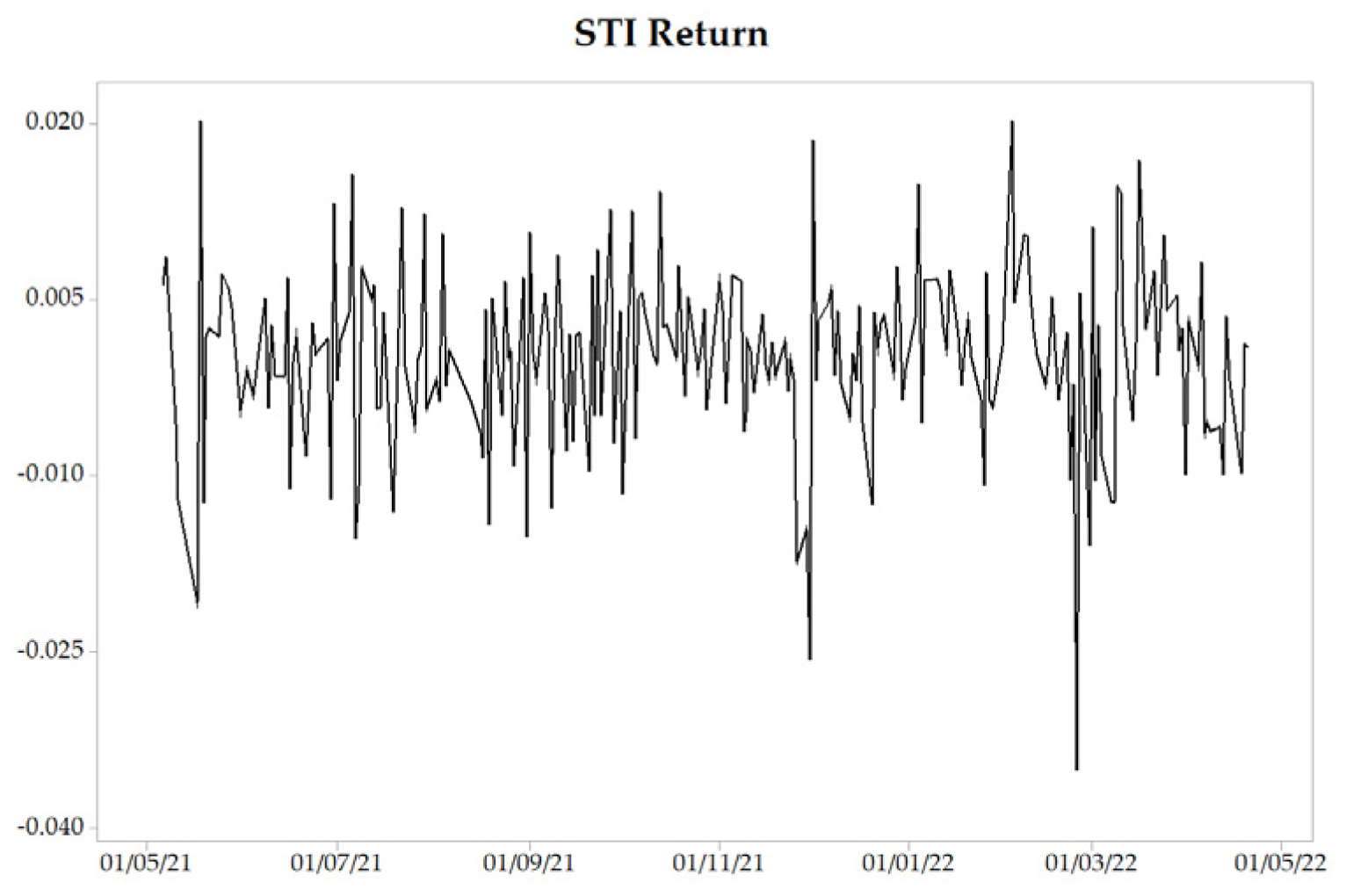
Figure 1 shows the return values of the ASEAN top five stock price indexes.
Referring to Figure 1, the graph of the return value had stationary movement, and no drastic changes were found. This condition indicated that the market conditions tended to be normal with stable profits.

4.1. Stock Price Index Modeling with GBM Model

In the GBM model, there is a requirement that the return value must be normally distributed (Widyarti et al. 2021). Therefore, it was necessary to test for normality before compiling the model and determining the predictive value. The data normality test method chosen was Jarque–Bera. The Jarque–Bera method was chosen because it is superior in power to its competitors for symmetric distributions with medium to long tails and slightly skewed distributions with long tails (Desgagné and Lafaye de Micheaux 2017). The following are the results of the normality test of data returns in the sample.
Normality testing in this study used α = 5%. Based on Table 4, for each stock price index return, a p-value > α was obtained so that all data were normally distributed (Hanusz and Tarasinska 2015). After the normality test was performed, the following procedure was used to determine the parameter values of the GBM model, which included the return mean (μ), volatility (σ), and time change (Δt).
The selection of Δt = 1 day, based on the shortest period of stock price index recording available and the shorter changes in the time used, will help investors find possible price conditions and profits in the near future (Abraham et al. 2018). By inserting the parameter values from Table 5 into Equation (8), the GBM models for each country are:
  • Indonesia (JKSE)
    S p i = S p i 1 exp 7.4315 × 10 4 5.56 × 10 4 2 + ( 7.4572 × 10 3 ) Z i 1
  • Philippines (PSEI)
    S p i = S p i 1 exp 5.5682 × 10 4 1.63 × 10 4 2 + ( 1.2796 × 10 2 ) Z i 1
  • Malaysia (KLSE)
    S p i = S p i 1 exp 3 × 10 4 6.19 × 10 5 2 + ( 7.866 × 10 3 ) Z i 1
  • Thailand (SET)
    S p i = S p i 1 exp 3.87 × 10 3 5.11 × 10 5 2 + ( 7.147 × 10 3 ) Z i 1
  • Singapore (STI)
    S p i = S p i 1 exp 2.8257 × 10 4 6.07 × 10 5 2 + ( 7.7894 × 10 3 ) Z i 1
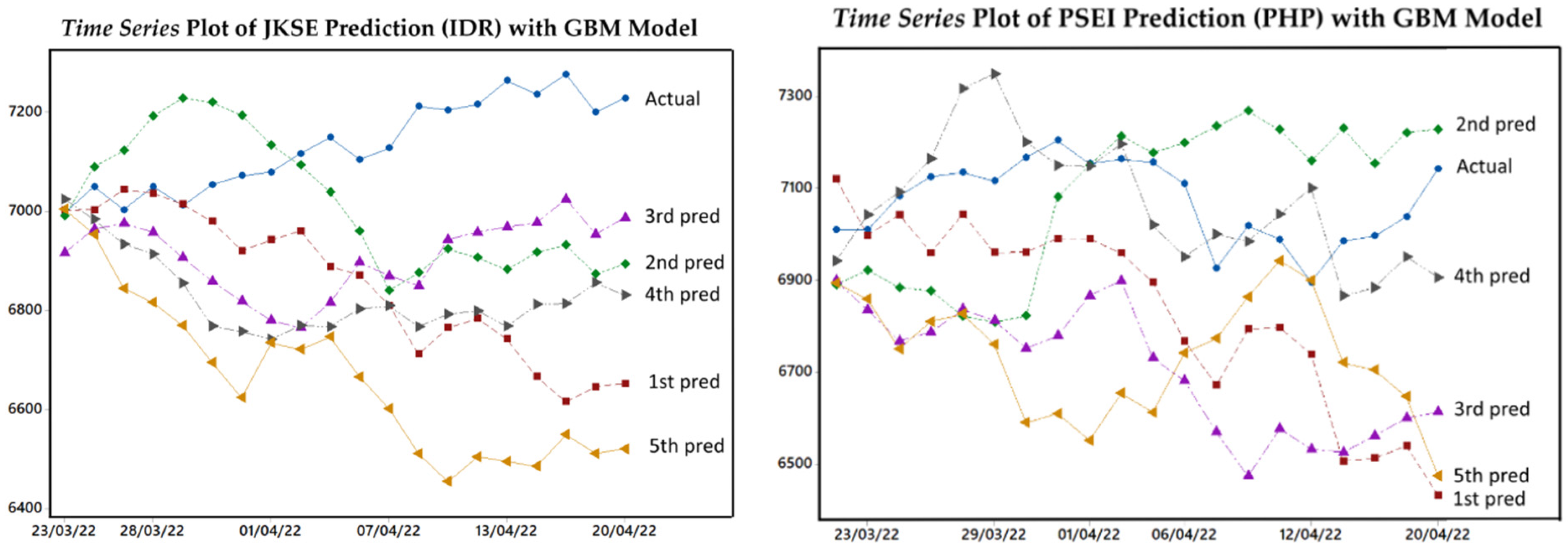
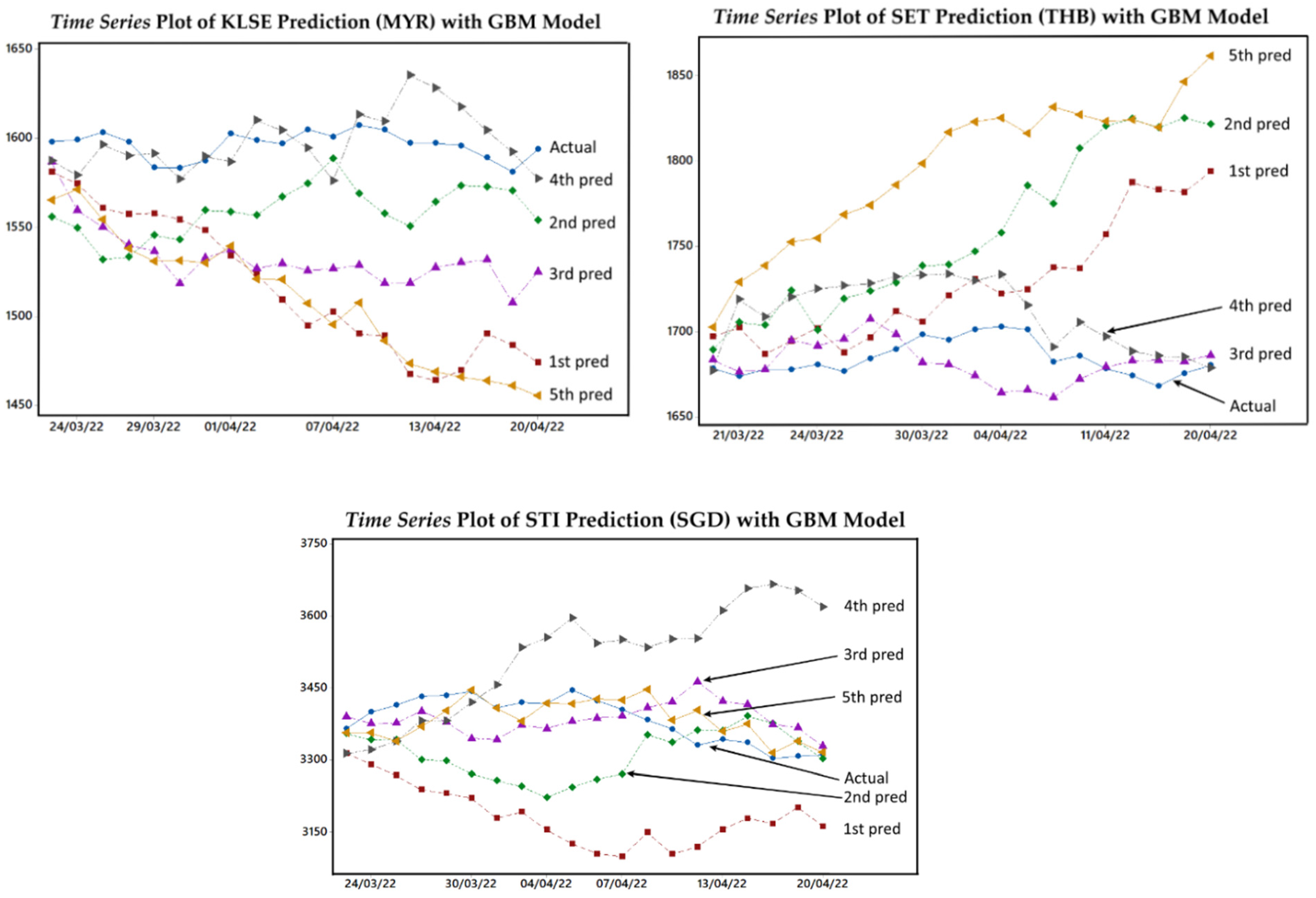
The GBM model for each country was used to predict the stock price index value for the next 20 periods. In each country, prediction experiments were carried out five times without repetition. The following is a plot of the prediction results and MAPE values for each country, starting from the 1st to the 5th prediction experiment on the out-sample data (20 periods).
In Figure 2, each experiment’s predicted results were significantly different (unstable). This result was unsatisfactory as a guide for investors to predict the future estimated value of the price index. It is well known that in economics and financial investment, a statistical model is expected to provide accurate and stable results (Siami-Namini et al. 2018). Only with excellent and stable accuracy results can investment strategies in the future be well prepared and help to provide optimal profit (Hsu et al. 2016). Unstable GBM modelling results were found in the research conducted by Ramos et al. (2019) and Mosino and Moreno-Okuno (2018). They used the GBM model to predict iron ore and fossil fuel prices, where the GBM model had limitations in providing convergent prediction results. Furthermore, the following are the MAPE values for the prediction results for each stock price index.
Based on the MAPE values in Table 6, the prediction results proved unstable because the MAPE values obtained were still significantly different in each experiment. To overcome this limitation, the GBM-MCS model was used.

4.2. Stock Price Index Modelling Using GBM-MCS

In the GBM-MCS model, there is an iterative process that aims to obtain different possible results in each experiment (Maruddani and Trimono 2018). After repeating it m times, we determined the average value to obtain a single prediction result. The more repetitions, the more convergent the results will be (Soleimani et al. 2020). In this study, the repetition was carried out 5000 times. The results are shown in Table 7.
Theoretically, the GBM-MCS model could provide more stable and accurate results than the GBM model. In Table 7, for m = 5000, the highest predictive value for JKSE was IDR 7304.5 on 18/04, and the smallest predictive value was IDR 6962.43 on 29/03. For PSEI, the highest prediction occurred on 30/03 with a value of 7289.9, while the lowest occurred in the following six periods on 07/04 with a value of 6801.05. The price prediction for the Malaysian state stock index was MYR 1560–1660. The highest value was recorded on 01/04/22, MYR 1658.72, while the lowest predicted value occurred on 14/04 at MYR 1560.61. The SET stock price index prediction results were the most stable among other stock price indexes because they have the smallest volatility value, with a value of 0.00935. Then, the STI stock price index, which measures the stability of the prediction results, was the best after SET. The recorded volatility value was 0.01625. Thus, based on the prediction results, investors are suggested to invest in the stock markets of Thailand and Singapore because the stock prices are stable, which will minimize the risk of losses.
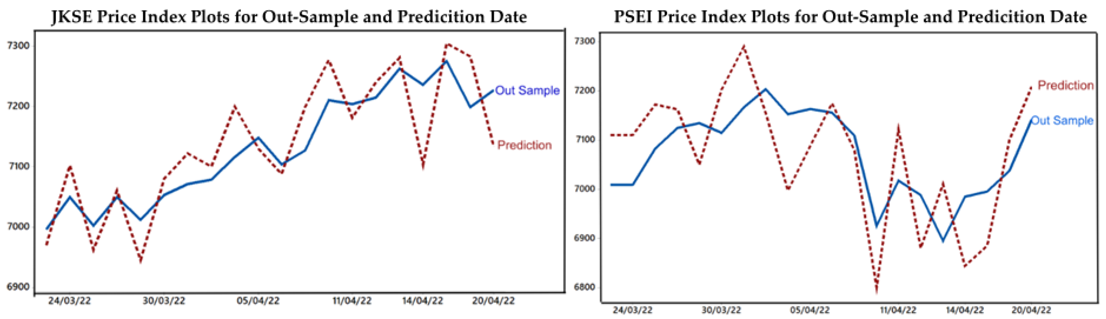
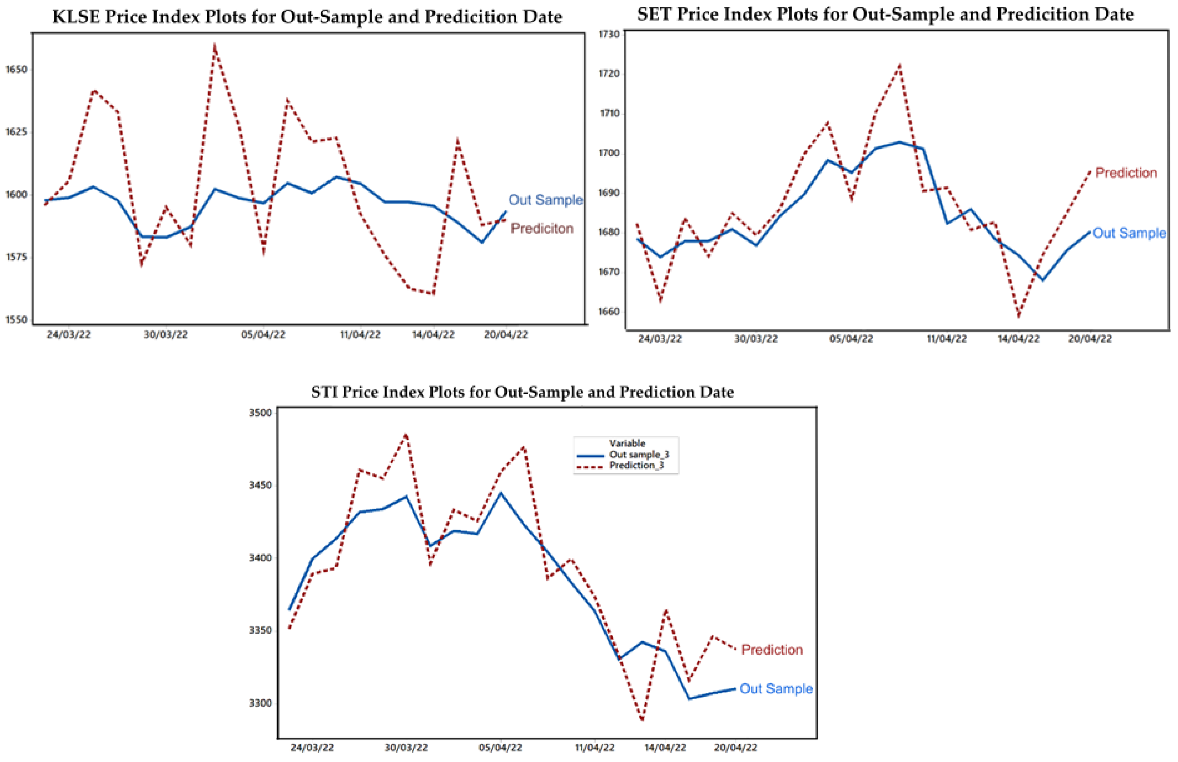
To make it easier to compare the actual and predicted values of GBM-MCS (m = 500), the following is a comparison of the two values using a time-series graph.
A good prediction must have the slightest difference between the actual and predicted values (high accuracy) (Nguyen et al. 2015). The comparison plot in Figure 3 shows that the predicted price was relatively close to the actual price, meaning that graphically, the GBM-MCS model provided accurate prediction results. Using the MAPE values, the following is the accuracy obtained:
Based on the MAPE values in Table 8, all calculation results were within the “very accurate” category, thus providing more stable predictions than the GBM model. These results indicated that the GBM-MCS model could effectively be used as the price index prediction method for the stock market in the ASEAN. For investors investigating the condition of stock price movements and stock price indexes in the post-COVID-19 era, as the stock market in the ASEAN tends to be in a normal and stable condition, the GBM-MCS model is more recommended than other models. The Table 9 is the predicted value of the stock price index for the period after the out-sample data.
The Monte Carlo simulation that was used to predict the stochastic models was proven to improve the accuracy. Marchenko and Cherepovitsyn (2017) applied the Monte Carlo simulation to the NPV model to evaluate mining investment projects, and concluded that it gives a more accurate approximation of the possible uncertainty about the projected results of the investment projects. Pan and Dias (2017)investigated the efficiency of the Monte Carlo simulation combined with the adaptive support vector machine (ASVM) model. The MCS was employed to compute the failure probability based on the SVM classifier obtained. The proposed method was applied to four representative examples, which indicated the effectiveness and efficiency of ASVM-MCS, leading to accurate failure probability estimations with a relatively low computational cost.

4.3. Risk Prediction

VaR is an appropriate risk measure that is used when the market is under normal conditions(Abad et al. 2014). VaR is expected to be a valid reference for investors to determine the estimated risk of loss for investments that are being carried out (Fissler and Ziegel 2021). The data used were the values of the stock price index predicted in the out-sample period with the GBM-MCS model. VaR, with the variance–covariance approach, measures the return value. The following are descriptive statistics of the stock price index returns predicted in the out-sample period.
Table 10 shows that JKSE, PSEI, and SET had positive returns, while KLSE and STI had negative returns. The negative values illustrated that during that period, in general, stocks in the stock markets of Malaysia and Singapore experienced losses. Furthermore, the mean and standard deviation were used to predict the risk of loss using the VaR-VC method. Based on the date 20/04/2022 as a reference, the results of the risk predictions at various confidence levels and holding periods are presented in the following table.
The prediction results shown in Table 11 show that a risk of loss might occur between −0.01 and 0.15. This value was relatively small, so investing in the stock market in five countries was safe for novice and large-scale investors. For each level of confidence and holding period, the stock price indexes of the Philippines (PSEI) and Malaysia (KLSE) tended to have the most significant risk of loss, which was greater than in other countries. On the other hand, the Thai stock price index (SET) showed the lowest risk prediction value among all countries. As an example of the interpretation of Table 10, the VaR-VC value for JKSE at a 95% confidence level (α = 5%) and a 3-day holding period was −0.0444. The predicted maximum loss for the following three periods since 20/04/2022 was 4.44% of the total invested funds.
In addition to the potential profit, the risk of loss is also an important consideration in investing. Based on the calculations of the VaR values, the stock market that was most recommended for investment was SET. In addition to the slightest risk of loss, based on modeling using GBM-MCS, the value of the SET stock price index was also the most stable among the stock price indexes of other countries. The practical implications based on the results of stock price indexes and loss risk predictionsare that this model can directly be a reference for investors to choose which stock market to invest in. The most ideal stock market to invest in is SET (Thailand), because it has the smallest loss risk value compared to the other markets. Then, the managerial implications from this research enable it to be a guideline for determining the best risk management strategy so that the investments that have been made in the stock market can provide optimal benefits.

5. Conclusions

The stock price index valuation, which includes the prediction of the price index and the risk of loss in the ASEAN top five countries, concluded that the GBM-MCS model is more accurate for modeling the value of the price index in the future than the GBM model. This conclusion refers to the MAPE value of the GBM-MCS model, which is more stable than the GBM model.
In predicting the risk of loss through the VaR-VC model, it is known that the possible losses that will occur for the next one, three, and five periods are in the interval of 1–15%. This relatively small loss prediction value can be a justification that the stock market in the ASEAN top five countries is the right choice for novice investors who want a small risk with stable profits in the new normal era.
The limitation of this research is related to the assumption of normality of the data, which causes the number of periods used for the analysis to be limited so that the assumption of normality is still met. Therefore, in future research, we suggest using the GBM with the jump (jump diffusion) model. This model is a development of the GBM that does not suggest the assumption of normality, making it possible for us to use more periods.

Author Contributions

Conceptualization, H.H.; Methodology, E.T.W., D.A.I.M. and T.T.; Investigation, H.H.; Data curation, D.A.I.M.; Writing—original draft, H.H.; Writing—review & editing, D.A.I.M.; Project administration, T.T. All authors have read and agreed to the published version of the manuscript.

Funding

This research was funded by Diponegoro University, grant number 185-03/UN7.6JPP/2022.

Conflicts of Interest

The authors declare no conflict of interest.

References

  1. Abad, Pilar, Sonia Benito, and Carmen López. 2014. A comprehensive review of Value at Risk methodologies. Spanish Review of Financial Economics 12: 15–32. [Google Scholar] [CrossRef]
  2. Abidin, Siti Nazifah Zainol, and Maheran Mohd Jaffar. 2014. Forecasting Share Prices of Small Size Companies in Bursa Malaysia Using Geometric Brownian Motion. Applied Mathematics & Information Sciences 8: 107–12. [Google Scholar] [CrossRef] [Green Version]
  3. Abraham, Jethin, Daniel Higdon, John Nelson, and Juan Ibarra. 2018. SMU Data Science Review Cryptocurrency Price Prediction Using Tweet Volumes and Sentiment Analysis Cryptocurrency Price Prediction Using Tweet Volumes and Sentiment Analysis. SMU Data Science Review 1: 1–22. [Google Scholar]
  4. Adamu, Jamilu Auwalu. 2018. IFRS 9 Measurement of Financial Instruments 2018: Jameel’s Non-Normal Brownian Motion Models Are Indeed IFRS 9 Complaint Models. Journal of Economics and Management Sciences 1: 1–22. [Google Scholar] [CrossRef] [Green Version]
  5. Adrian, Tobias, Erkko Etula, and Tyler Muir. 2014. Financial Intermediaries and the Cross-Section of Asset Returns. The Journal of Finance 69: 2557–96. [Google Scholar] [CrossRef]
  6. Algalith, Moawia. 2017. Stochastic optimization without Ito’s lemma: Applications to the portfolio model. Economics Bulletin 37: 2533–36. [Google Scholar]
  7. Ali, Basel J. A., and Mohammad Salem Oudat. 2020. Financial Risk and The Financial Performance in Listed Commercial and Investment Banks in Bahrain Bourse. International Journal of Innovation, Creativity and Change 13: 160–80. [Google Scholar]
  8. Angelaccio, Michele. 2019. Forecasting Public Electricity Consumption with ARIMA Model: A Case Study from Italian Municipalities Energy Data. Paper presented at the 2019 International Symposium on Advanced Electrical and Communication Technologies, Rome, Italy, November 27–29. [Google Scholar] [CrossRef]
  9. Antwi, Osei, Kyere Bright, and Kwasi Awuah Wereko. 2020. Jump Diffusion Modeling of Stock Prices On Ghana Stock Exchange. Journal of Applied Mathematics and Physics 8: 1736–54. [Google Scholar] [CrossRef]
  10. Arisandhi, Vicho Dwindra, and Robiyanto Robiyanto. 2022. Exchange Rate, Gold Price, And Stock Price Correlation in Asean-5: Evidence From COVID-19 Era. Jurnal Manajemen Dan Kewirausahaan 24: 22–32. [Google Scholar] [CrossRef]
  11. ASEAN Biodiaspora Virtual Center. 2020. COVID-19 Situational Report in the ASEAN+3 Region. Jakarta: ASEAN Press. [Google Scholar]
  12. ASEAN Biodiaspora Virtual Center. 2021. COVID-19 Situational Report in the ASEAN+3 Region. Jakarta: ASEAN Press. [Google Scholar]
  13. ASEAN Secretariat. 2019. ASEAN Investment Report 2019: FDI in Service: Focus on Health Care. Jakarta: ASEAN Secretariat. [Google Scholar]
  14. ASEAN Secretariat. 2021. ASEAN Investment Report 2020–2021: Investing in Industry 4.0. Jakarta: ASEAN Secretariat. [Google Scholar]
  15. ASEAN Secretariat. 2022. ASEAN Investment Report 2022: Pandemic Recovery and Investment Facilitation. Jakarta: ASEAN Secretariat. [Google Scholar]
  16. Aziz, Mukhriz Izraf Azman, Norzalina Ahmad, Jin Zichu, and Safwan Mohd Nor. 2022. The Impact of COVID-19 on the Connectedness of Stock Index in ASEAN+ 3 Economies. Mathematics 10: 1417. [Google Scholar] [CrossRef]
  17. Basson, Lisa M., Peter J. Kilbourn, and Jackie Walters. 2019. Forecast Accuracy in Demand Planning: A Fast-Moving Consumer Goods Case Study. Journal of Transport and Supply Chain Management 13: 1–9. [Google Scholar] [CrossRef] [Green Version]
  18. Blanchard, Olivier. 2019. Public Debt and Low Interest Rates. American Economic Review 109: 1197–229. [Google Scholar] [CrossRef]
  19. Bratin, Vasile, Ana-Maria Acu, Diana Marieta Mihaiu, and Radu-Alexandru Serban. 2022. Geometric Brownian Motion (GBM) of Stock Indexes and Financial Market Uncertainty in the Context of Non-Crisis and Financial Crisis Scenarios. Mathematics 2022: 309. [Google Scholar] [CrossRef]
  20. Budiarso, Novi Swandari, Abdul Wahab Hasyim, Rusman Soleman, Irfan Zam Zam, and Winston Pontoh. 2020. Investor Behavior Under The COVID-19 Pandemic: The Case of Indonesia. Investment Management and Financial Innovations 17: 308–18. [Google Scholar] [CrossRef]
  21. Bustos, Oscar, and Alexandra Pomares-Quimbaya. 2020. Stock Market Movement Forecast: A Systematic Review. Expert Systems with Applications 156: 113464. [Google Scholar] [CrossRef]
  22. Celik, Ismail, Tayfun Yilmaz, Süleyman Emir, and Ahmet Furkan Sak. 2020. The effects of COVID-19 outbreak on financial markets. Financial Studies 24: 6–28. [Google Scholar]
  23. Chaengkham, Supakorn, and Suthin Wianwiwat. 2021. Stock Market Index Prediction Using Machine Learning: Evidence from Leading Southeast Asian Countries. Thailand and The World Economy 39: 56–64. [Google Scholar]
  24. Chien, Feng Sheng, Muhammad Sadiq, Hafiz Waqas Kamran, Muhammad Atif Nawaz, Muhammed Sajjad Hussain, and Muhammad Raza. 2021. Co-Movement of Energy Prices and Stock Market Return: Environmental Wavelet Nexus of COVID-19 Pandemic from the USA, Europe, and China. Environmental Science and Pollution Research 28: 32359–73. [Google Scholar] [CrossRef] [PubMed]
  25. Chong, Terence Tai Leung. 2021. The impact of COVID-19 on ASEAN. Economic and Political Studies 9: 166–85. [Google Scholar] [CrossRef]
  26. Chu, Zhong, Zhengwei Wang, Jing Jian Xiao, and Weiqiang Zhang. 2017. Financial Literacy, Portfolio Choice, and Financial Well-Being. Social Indicators Research 132: 799–820. [Google Scholar] [CrossRef] [Green Version]
  27. Chudy, R. P., and F. W. Gubbage. 2020. Research trends: Forest investments as a financial asset class. Forest Policy and Economics 119: 102273. [Google Scholar] [CrossRef] [PubMed]
  28. Davies, Robert, Tim Coole, and David Osipyw. 2014. The Application of Time Series Modelling and Monte Carlo Simulation: Forecasting Volatile Inventory Requirements. Scientific Research 5: 1152–68. [Google Scholar] [CrossRef] [Green Version]
  29. Degutis, Augustas, and Lina Novickytė. 2014. The Efficient Market Hypothesis: A Critical Review of Literature and Methodology. Ekonomika 93: 7–23. [Google Scholar] [CrossRef] [Green Version]
  30. Desgagné, Alain, and P. Lafaye de Micheaux. 2017. A Powerful and Interpretable Alternative to The Jarque–Bera Test of Normality Based on 2nd-Power Skewness And Kurtosis, Using The Rao’s Score Test On The APD Family. Journal of Applied Statistics 45: 2307–27. [Google Scholar] [CrossRef]
  31. Dionne, Georges. 2013. Risk management: History, definition, and critique. Risk Management and Insurance Review 16: 147–66. [Google Scholar] [CrossRef] [Green Version]
  32. Doshi, Hitesh, Praveen Kumar, and Vijay Yerramilli. 2015. Uncertainty, Capital Investment, And Risk Management. Management Science 64: 5769–86. [Google Scholar] [CrossRef] [Green Version]
  33. Estemner, Rene, and Michael John Marana. 2016. Forecasting of Stock Prices Using Brownian Motion—Monte Carlo Simulation. Paper presented at the 2016 International Conference on Industrial Engineering and Operations Management, Kuala Lumpur, Malaysia, March 8–10; pp. 704–13. [Google Scholar]
  34. Fissler, Tobias, and Johanna Ziegel. 2021. On the elicitability of range value at risk. Statistics & Risk Modeling 38: 25–46. [Google Scholar] [CrossRef]
  35. Hamdan, Zawin Najah, S. N. I. Ibrahim, and MohdShafie Mustafa. 2020. Modelling Malaysian Gold Prices Using Geometric Brownian Motion Model. Advances in Mathematics: Scientific Journal 9: 7463–69. [Google Scholar] [CrossRef]
  36. Hanusz, Zofia, and Joanna Tarasinska. 2015. Normalization of the Kolmogorov–Smirnov and Shapiro–Wilk tests of normality. Biometric Letters 52: 85–93. [Google Scholar] [CrossRef] [Green Version]
  37. Haseeb, Muhammad, Samanan Wattanapongphasuk, and Kittisak Jermsittiparsert. 2019. Financial Development, Market Freedom, Political Stability, Economic Growth and CO2 Emissions: An Unexplored Nexus in ASEAN Countries. Contemporary Economics 13: 363–74. [Google Scholar] [CrossRef]
  38. Hersugondo, Hersugondo, Imam Ghozali, Eka Handriani, Trimono Trimono, and Imang Dapit Pamungkas. 2022. Price Index Modeling and Risk Prediction of Sharia Stocks in Indonesia. Economies 10: 17. [Google Scholar] [CrossRef]
  39. Hsu, Ming-Wei, Stefan Lessmann, Ming-Chien Sung, Tiejun Ma, and Johnnie E. V. Johnson. 2016. Bridging the Divide In Financial Market Forecasting: Machine Learners Vs. Financial Economists. Expert Systems with Applications 61: 215–34. [Google Scholar] [CrossRef] [Green Version]
  40. Joshipura, Mayank, and Nehel Joshipura. 2020. Low-risk effect: Evidence, explanations, and approaches to enhancing the performance of lowrisk investment strategies. Investment Management and Financial Innovations 17: 128–45. [Google Scholar] [CrossRef]
  41. Kumar, Munish, Surbhi Gupta, Krishan Kumar, and Monika Sachdeva. 2020. Spreading Of COVID-19 In India, Italy, Japan, Spain, UK, US: A Prediction Using Arima and Lstm Model. Digital Government: Research and Practice 1: 1–9. [Google Scholar] [CrossRef]
  42. Lee, Chul-Yong, and Jaekyun Ahn. 2020. Stochastic Modeling of The Levelized Cost of Electricity for Solar PV. International Review of Automatic Control 13: 3017. [Google Scholar] [CrossRef]
  43. Lee, Siaw Li, Chin Ying Liew, Chee Khium Chen, and Li Li Voon. 2022. Geometric Brownian Motion-Based Time Series Modeling Methodology for Statistical Autocorrelated Process Control: Logarithmic Return Model. International Journal of Mathematics and Mathematical Sciences 2022: 1–10. [Google Scholar] [CrossRef]
  44. Liu, Lu, Junbing Huang, and Hong Li. 2022. Estimating the real shock to the economy from COVID-19: The exampleof electricity use in China. Technological and Economic Development of Economy 28: 1221–41. [Google Scholar] [CrossRef]
  45. Malarvizhi, Chinnasamy Agamudai Nambhi, Yashar Zeynali, Abdullah Al Mamun, and Ghazali Bin Ahmad. 2019. Financial Development and Economic Growth In ASEAN-5 Countries. Global Business Review 20: 57–71. [Google Scholar] [CrossRef]
  46. Marchenko, Roman S., and Alexey E. Cherepovitsyn. 2017. Improvement of the Quality of Calculations Using the Monte Carlo Simulation Method in The Evaluation of Mining Investment Projects. Paper presented at the 2017 International Conference “Quality Management, Transport and Information Security, Information Technologies”, IT and QM and IS, St. Petersburg, Russia, September 24–30; pp. 247–51. [Google Scholar] [CrossRef]
  47. Maruddani, Di Asih I., and Trimono. 2018. Modeling Stock Prices in A Portfolio Using Multidimensional Geometric Brownian Motion. Journal of Physics: Conference Series 1025: 012122. [Google Scholar] [CrossRef]
  48. Michaelsen, Markus, and Alexander Szimayer. 2018. Marginal Consistent Dependence Modeling Using Weak Subordination for Brownian Motions. SSRN Electronic Journal 2016: 1–26. [Google Scholar] [CrossRef]
  49. Miskolczi, Panna. 2017. Note on simple and logarithmic return. Applied Studies in Agribusiness and Commerce 11: 127–36. [Google Scholar] [CrossRef]
  50. Mosino, Alejandro, and Alejandro Tatsuo Moreno-Okuno. 2018. On modeling fossil fuel prices: Geometric Brownian motion vs. variance-gamma process. Economics Bulletin 38: 509–19. [Google Scholar]
  51. Nguyen, Thien Hai, Kiyoaki Shirai, and Julien Velcin. 2015. Sentiment Analysis On Social Media For Stock Movement Prediction. Expert Systems with Applications 42: 9603–11. [Google Scholar] [CrossRef]
  52. Organisation for Economic Co-operation and Development (OECD). 2021. Economic Outlook for Southeast Asia, China, and India 2020: Rethinking Education for the Digital Era. Paris: OECD Publishing. [Google Scholar] [CrossRef]
  53. Pan, Qiujing, and Daniel Dias. 2017. An Efficient Reliability Method Combining Adaptive Support Vector Machine and Monte Carlo Simulation. Structural Safety 67: 85–95. [Google Scholar] [CrossRef]
  54. Parungrojrat, Nopmanee, and Akaranant Kidsom. 2019. Stock Price Forecasting: Geometric Brownian Motion and Monte Carlo Simulation Techniques. MUT Journal of Business Administration 16: 9–103. [Google Scholar]
  55. Peng, Shige. 2019. Nonlinear Expectations and Stochastic Calculus under Uncertainty. Berlin: Springer. [Google Scholar]
  56. Purnaningrum, Evita, and Rina Fariana. 2022. Dynamic Ensemble Time Series For Prediction Major Indices In Asean. Indonesian Journal of Social Research (IJSR) 4: 54–62. [Google Scholar] [CrossRef]
  57. Ramadan, Helmi, Prana Ugiana Gio, and Elly Rosmaini. 2020. Monte Carlo Simulation Approach To Determine The Optimal Solution of Probabilistic Supply Cost. Journal of Research in Mathematics Trends and Technology 2: 1–6. [Google Scholar] [CrossRef]
  58. Ramos, André Lubene, Douglas Batista Mazzinghy, Viviane da Silva Borges Barbosa, Michel Melo Oliveira, and Gilberto Rodrigues da Silva. 2019. Evaluation of an Iron Ore Price Forecast Using a Geometric Brownian Motion Model. Revista Escola de Minas 72: 9–15. [Google Scholar] [CrossRef] [Green Version]
  59. Rathnayaka, R. M. Kapila Tharanga, Wei Jianguo, and D. M. K. N. Seneviratna. 2014. Geometric Brownian Motion with Ito’s Lemma Approach to Evaluate Market Fluctuations: A Case Study on Colombo Stock Exchange. Paper presented at the 2014 IEEE International Conference on Behavioral, Economic, Socio-Cultural Computing, BESC 2014, Shanghai, China, October 30–November 1. [Google Scholar]
  60. Reddy, Krishna, and Vaughan Clinton. 2016. Simulating Stock Prices Using Geometric Brownian Motion: Evidence from Australian Companies. Australasian Accounting, Business and Finance Journal 10: 23–47. [Google Scholar] [CrossRef] [Green Version]
  61. Rizvi, Syed Aun R., Solikin M. Juhro, and Paresh K. Narayan. 2021. Understanding Market Reaction To COVID-19 Monetary and Fiscal Stimulus in Major Asean Countries. Bulletin of Monetary Economics and Banking 24: 314–34. [Google Scholar] [CrossRef]
  62. Sako, Dumnamene, ChimaIgiri G. Igiri, and I. N. Chikweri. 2017. An Effective Tool for the Management of Stock Portfolio Using Variance-Covariance Approach of Value at Risk Models. International Journal of Computer Science and Mathematical Theory 3: 71–81. [Google Scholar]
  63. Siami-Namini, Sima, Neda Tavakoli, and Akbar SiamiNamin. 2018. A Comparison of ARIMA and LSTM in Forecasting Time Series. Paper presented at the 17th IEEE International Conference on Machine Learning and Applications, ICMLA 2018, Orlando, FL, USA, December 17–20; pp. 1394–401. [Google Scholar] [CrossRef]
  64. Sinha, Amit. 2021. The reliability of geometric Brownian motion forecasts of S&P500 index values. Journal of Forecasting 40: 1444–62. [Google Scholar] [CrossRef]
  65. Soleimani, Hamed, Omid Nasri, Mahbobehv Ghoochani, Abooalfazl Azhdarpoor, Mansooreh Dehghani, Majid Radfard, Mohammad Darvishmotevalli, Vahide Oskoei, and Maryam Heydari. 2020. Groundwater Quality Evaluation and Risk Assessment of Nitrate Using Monte Carlo Simulation and Sensitivety Analysis in Rural Areas of Divandarreh County, Kurdistan Province, Iran. International Journal of Environmental Analytical Chemistry 102: 1–19. [Google Scholar] [CrossRef]
  66. Stojkoski, Viktor, Trifce Sandev, Lasko Basnarkov, Lupco Kocarev, and Ralf Metzler. 2020. Generalised Geometric Brownian Motion: Theory and Applications to Option Pricing. Entropy 22: 1432. [Google Scholar] [CrossRef] [PubMed]
  67. Suci, Stannia Cahaya, Alla Asmara, and Sri Mulatsih. 2015. The Impact of Globalization On Economic Growth In ASEAN. Bisnis&Birokrasi, JurnalIlmuAdministrasi Dan Organisasi 22: 79–87. [Google Scholar] [CrossRef]
  68. Suriyankietkaew, Suparak, and Suthep Nimsai. 2021. COVID-19 Impacts and Sustainability Strategies for Regional Recovery in Southeast Asia: Challenges and Opportunities. Sustainability 13: 8907. [Google Scholar] [CrossRef]
  69. Thaler, Denny, Leonard Elezaj, Franz Bamer, and Bernd Markert. 2022. Training Data Selection for Machine Learning-Enhanced Monte Carlo Simulations In Structural Dynamics. Applied Sciences 12: 581. [Google Scholar] [CrossRef]
  70. Thapa, Prabin, and Binil Aryal. 2021. Use Of Geometric Brownian Motion To Forecast Stock Market Scenario Using Post COVID-19 NEPSE Index. Bibechana 18: 50–60. [Google Scholar] [CrossRef]
  71. Tubikanec, Irene, Massimiliano Tamborrino, Petr Lansky, and Evelyn Buckwar. 2022. Qualitative properties of different numerical methods for the inhomogeneous geometric Brownian motion. Journal of Computational and Applied Mathematics 406: 1–29. [Google Scholar] [CrossRef]
  72. Ullah, Sabeeh. 2022. Impact of COVID-19 Pandemic on Financial Markets: A Global Perspective. Journal of the Knowledge Economy 13: 1–22. [Google Scholar] [CrossRef]
  73. Walter, Christian. 2021. The Brownian Motion in Finance: An Epistemological Puzzle. Topoi 40: 793–809. [Google Scholar] [CrossRef]
  74. Wang, Qiuyun, and Lu Liu. 2022. Pandemic or Panic? A Firm-Level Study on the Psychological and IndustrialImpacts of COVID-19 on the Chinese Stock Market. Financial Innovation 8: 1–38. [Google Scholar] [CrossRef] [PubMed]
  75. Widyarti, Endang Tri, Di Asih I Maruddani, T. Trimono, and H. Hersugondo. 2021. Blue Chip Stocks Valuation and Risk Prediction on The Indonesia Stock. Academy Occounting and Financial Studies Journal 25: 1–14. [Google Scholar]
  76. Yuliadi, Imamudin, and Wahdi Salasi April Yudhi. 2021. Economic Growth Determinants OfAsean Economic Community: Feasible Generalized Least Square Approach. E3S Web of Conferences 316: 01019. [Google Scholar] [CrossRef]
  77. Yunita, Yunita, and Robiyanto Robiyanto. 2018. The Influence of Inflation Rate, Bi Rate, And Exchange Rate Changes to The Financial Sector Stock Price Index Return In The Indonesian Stock Market. JurnalManajemen Dan Kewirausahaan 20: 80–86. [Google Scholar] [CrossRef]
  78. Yusoff, M. Y. B. M. 2021. Covid-19 Pandemic Outbreak: The Asean-5 Stock Market Short-Term And Long-Term Responses. Review of International Geographical Education Online 11: 1033–46. [Google Scholar]
  79. Zhang, Wei-Guo, Zhe Li, Yong-Jun Liu, and Yue Zhang. 2021. Pricing European Option Under Fuzzy Mixed Fractional Brownian Motion Model with Jumps. Computational Economics 58: 483–515. [Google Scholar] [CrossRef]
Figure 1. ASEAN-5 stock price index returns.
Ijfs 10 00112 g001aIjfs 10 00112 g001b
Figure 2. ASEAN top 5 stock price index predictions for next 20 periods with GBM model.
Ijfs 10 00112 g002aIjfs 10 00112 g002b
Figure 3. Out-sample stock price index comparison plots and predictions.
Ijfs 10 00112 g003aIjfs 10 00112 g003b
Table 1. General description for ASEAN-5stock price indexes.
CountryStock Price Index (Code)CurrencyTotal ObsIn-Sample DataOut-Sample Data
IndonesiaJakarta Composite Index (JKSE)IDR23421420
PhilippinesPhilippines Stock Exchange Index (PSEI)PHP23321320
MalaysiaKuala Lumpur Stock Exchange (KLSE)MYR23521520
ThailandStock Exchange Thailand (SET)THB23321320
SingaporeStrait Times Index (STI)SGD23521520
Table 2. Descriptive statistics of ASEAN top 5 stock price indexes.
JKSEPSEIKLSESETSTI
Mean6457.626999.641552.771625.953195.99
St. Dev383.28284.02735.5745.45105.06
Variance146,902.6580,671.511264.912065.4411,038.21
Min5760.586164.891480.921521.723041.29
Max7275.297502.481659.221713.203445.01
Skewness−0.04105−0.594690.10485−0.324261.06988
Kurtosis−1.39921−0.15153−0.81168−0.425610.82092
Table 3. Descriptive statistics of ASEAN top 5 stock price index returns.
JKSEPSEIKLSESETSTI
Mean0.000820.0003420.000050.000350.00021
Volatilities0.007320.0126910.007650.006930.00765
Variance0.000050.0001610.000060.000050.00006
Min−0.02078−0.04352−0.04457−0.02730−0.03507
Max0.020350.049810.035480.018430.02023
Skewness−0.07136−0.16557−0.40624−0.66140−0.60239
Kurtosis0.147171.989845.762671.514192.08011
Table 4. Jarque–Beranormality test result for ASEAN top 5 stock price index returns.
SchemeJKSEPSEIKLSESETSTI
JB0.30000.8700.8331.0491.022
p-value0.80690.4350.4910.2210.248
DecisionH0 acceptedH0 acceptedH0 acceptedH0 acceptedH0 accepted
Table 5. GBM model parameters.
ParametersJKSEPSEIKLSESETSTI
μ7.4315 × 10−45.5682 × 10−43 × 10−43.87 × 10−42.8257 × 10⁻⁴
σ7.4572 × 10−31.2796 × 10−27.866 × 10−37.147 × 10−37.7894 × 10⁻³
Δt1 day1 day1 day1 day1 day
Table 6. MAPE values for GBM model predictions.
MAPE (%)
JKSEPSEIKLSESETSTI
1st pred3.953.514.992.615.94
2nd pred2.832.582.334.382.75
3rd pred3.115.183.960.861.59
4th pred4.281.350.861.594.79
5th pred6.584.745.436.640.85
Table 7. ASEAN top 5 stock price index predictions using GBM-MCS with 5000 repetitions.
JKSEPSEIKLSESETSTI
PeriodPredPeriodPredPeriodPredPeriodPredPeriodPred
23/036970.2122/037109.9423/031595.9118/031682.3923/033351.57
24/037102.2223/037110.4324/031605.8921/031663.1624/033389.26
25/036962.4324/037172.6125/031642.2322/031683.6625/033393.24
28/037060.3525/037162.2328/031633.3223/031674.1428/033461.09
29/036945.3428/037050.3929/031572.9124/031684.9229/033455.19
30/037080.2129/037202.8230/031595.2125/031679.4130/033485.92
31/037121.9930/037289.931/031580.2828/031686.1231/033396.69
01/047100.4331/037155.2501/041658.7229/031699.8101/043433.57
04/047199.8201/046997.2304/041627.2130/031707.7404/043425.72
05/047129.9204/047088.8505/041578.2831/031688.7305/043459.79
06/047088.0105/047175.0206/041637.8301/041710.3806/043477.23
07/047199.7306/047079.4307/041621.4104/041722.0607/043386.24
08/047276.8207/046801.0508/041622.8205/041690.6508/043399.82
11/047181.8808/047121.9111/041592.4107/041691.3811/043373.57
12/047240.4211/046880.8112/041575.8508/041680.812/043333.38
13/047280.5112/047010.3113/041562.8211/041682.6813/043287.91
14/047104.0813/046844.2414/041560.6112/041659.3414/043364.79
18/047304.518/046885.3215/041621.2718/041674.518/043316.02
19/047283.2219/047099.8918/041588.2819/041685.1219/043346.32
20/047133.6220/047208.7820/041590.1120/041695.6420/043337.43
Table 8. MAPE values (%) for GBM-MCS model predictions.
JKSEPSEIKLSESETSTI
MAPE0.66831.26340.68750.48010.6674
Table 9. ASEAN top 5 stock price index predictions for 21/04/22–18/05/22.
PeriodJKSEPSEIKLSESETSTI
21/047035.506961.371593.391675.603358.25
22/047069.566927.091593.221693.503320.87
25/047077.136917.891574.751684.743355.35
26/047016.616983.961591.201690.493366.33
27/047046.547070.891595.381682.023388.81
28/046921.097092.091607.741673.663406.91
29/046949.457070.441607.821666.053380.40
02/056991.667136.671606.841676.353393.68
03/057095.127214.461583.941655.243399.01
04/057133.617198.391610.331671.393366.47
05/057127.627104.691623.411668.533352.71
06/057178.027143.051622.421678.153356.80
09/057275.547099.171625.691671.623378.65
10/057254.607067.441640.481684.093344.19
11/057221.857022.021626.471680.363325.77
12/057247.746970.251642.691692.593286.48
13/057277.217105.451640.501686.483270.84
16/057258.657126.591628.031695.083287.28
17/057203.896903.561652.931685.133294.91
18/057114.616927.981666.281711.073280.13
Table 10. Descriptive statistics of stock price index prediction returns for out-sample period.
Returns of Stock Price Index Predictions
JKSEPSEIKLSESETSTI
Mean0.001220.00073−0.000190.00041−0.00022
St. dev0.015570.022740.023350.009240.01387
Minimum−0.02453−0.04012−0.03769−0.01841−0.02652
Maximum0.027820.046100.048440.012740.02311
Table 11. VaR-VC risk prediction results at various confidence levels and holding periods.
α = 10%α = 5%α = 1%
T = 1T = 3T = 5T = 1T = 3T = 5T = 1T = 3T = 5
JKSE−0.0200−0.0346−0.0446−0.0256−0.0444−0.0573−0.0362−0.0627−0.0810
PSEI−0.0291−0.0505−0.0652−0.0374−0.0648−0.0836−0.0529−0.0916−0.1183
KLSE−0.0299−0.0518−0.0669−0.0384−0.0665−0.0859−0.0543−0.0941−0.1215
SET−0.0118−0.0205−0.0265−0.0152−0.0263−0.0340−0.0215−0.0372−0.0481
STI−0.0178−0.0308−0.0397−0.0228−0.0395−0.0510−0.0323−0.0559−0.0721
Publisher’s Note: MDPI stays neutral with regard to jurisdictional claims in published maps and institutional affiliations.

