
Shrinking Working-Age Population and Food Demand: Evidence from Rural China


Abstract
:1. Introduction
2. Materials and Methods
2.1. Data
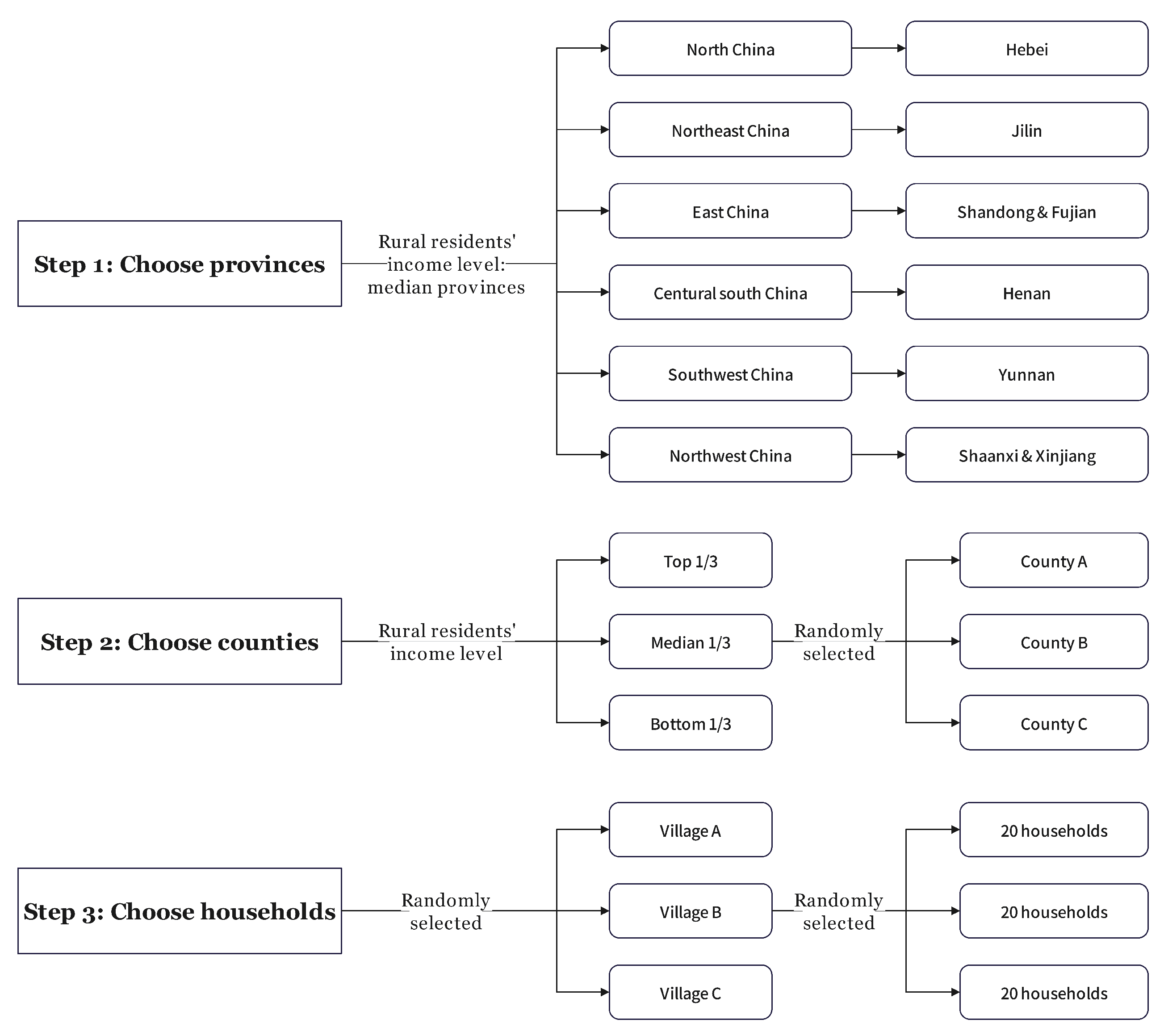
2.1.1. Data Source
2.1.2. Statistical Description
2.2. Econometric Model
2.2.1. Stage 1: The Working–Leser Model
2.2.2. Stage 2: The QUAIDS Model
2.2.3. Price Endogeneity
2.2.4. Demand Elasticity
3. Results
3.1. Model Estimation and Selection
3.2. Income Elasticity and Price Elasticity
3.3. Food Demand Elasticity among the Elderly Population
3.4. Income Elasticity of Food Demand among Elderly Populations with Different Income Levels
4. Discussion
5. Conclusions and Future Directions
Author Contributions
Funding
Institutional Review Board Statement
Informed Consent Statement
Data Availability Statement
Conflicts of Interest
Appendix A

| Category | Unit | WAP Strata | All | |||
|---|---|---|---|---|---|---|
| G1 0–60% | G2 60–65% | G3 65–70% | G4 70–100% | |||
| Per capita quantities consumed at home | ||||||
| Grain (GR) | Kg | 78.40 (61.12) | 75.08 (62.47) | 84.59 (61.42) | 87.18 (64.07) | 84.76 (63.28) |
| Oils and fats (OF) | Kg | 12.24 (8.07) | 11.87 (7.70) | 12.27 (8.21) | 13.80 (8.84) | 13.26 (8.62) |
| Animal products (AP) | Kg | 39.48 (32.32) | 35.19 (26.45) | 40.56 (29.61) | 43.86 (33.89) | 42.31 (32.94) |
| Fruits and vegetables (FV) | Kg | 61.66 (66.40) | 59.44 (57.12) | 62.85 (66.21) | 63.08 (66.99) | 62.64 (66.41) |
| Price (unit value) | ||||||
| Grain (GR) | CNY/kg | 5.12 (5.03) | 5.01 (4.91) | 4.88 (4.35) | 4.93 (4.27) | 4.96 (4.46) |
| Oils and fats (OF) | CNY/kg | 12.41 (6.90) | 12.47 (5.77) | 12.58 (6.76) | 13.35 (8.82) | 13.05 (8.17) |
| Animal products (AP) | CNY/kg | 20.52 (15.49) | 20.66 (11.52) | 21.14 (14.90) | 21.27 (14.57) | 21.09 (14.67) |
| Fruits and vegetables (FV) | CNY/kg | 5.00 (3.50) | 4.85 (2.87) | 5.34 (3.99) | 5.45 (4.47) | 5.33 (4.20) |
| Household characteristic | ||||||
| Per capita food expenditure | CNY 1000 | 1.37 (0.72) | 1.29 (0.70) | 1.47 (0.77) | 1.57 (0.79) | 1.51 (0.78) |
| Per capita total expenditure | CNY 1000 | 4.31 (2.45) | 4.08 (1.99) | 4.71 (2.46) | 5.15 (2.80) | 4.90 (2.70) |
| Proportion of the WAP | 0.36 (0.21) | 0.60 (0.01) | 0.67 (0.00) | 0.93 (0.11) | 0.78 (0.26) | |
| Observations | 2943 | 654 | 1824 | 10,476 | 15,897 | |
| Estimated Result | Bootstrap Standard Error | |
|---|---|---|
| 0.32 *** | (0.05) | |
| −0.03 *** | (0.00) | |
| Proportion of household WAP | 0.02 *** | (0.00) |
| Provincial dummy variables | Y | Y |
| Year dummy variables | Y | Y |
| Number of samples | 15,897 | 15,897 |
| Parameters | AIDS | QUAIDS1 | QUAIDS2 | QUAID3 |
|---|---|---|---|---|
| (1) | (2) | (3) | (4) | |
| 0.28 *** | 0.28 *** | 0.28 *** | 0.29 *** | |
| 0.10 *** | 0.10 *** | 0.10 *** | 0.11 *** | |
| 0.42 *** | 0.42 *** | 0.42 *** | 0.40 *** | |
| 0.19 *** | 0.19 *** | 0.20 *** | 0.20 *** | |
| −0.02 *** | −0.02 *** | −0.01 | −0.03 *** | |
| −0.04 *** | −0.04 *** | −0.04 *** | −0.04 *** | |
| 0.01 *** | 0.01 *** | 0.00 | 0.02 *** | |
| 0.05 *** | 0.05 *** | 0.05 *** | 0.04 *** | |
| 0.02 *** | 0.03 *** | 0.03 *** | 0.03 *** | |
| −0.02 *** | −0.02 *** | −0.02 *** | −0.01 *** | |
| −0.02 *** | −0.02 *** | −0.02 *** | −0.02 *** | |
| 0.01 *** | 0.01 *** | 0.01 *** | 0.01 *** | |
| 0.06 *** | 0.06 *** | 0.06 *** | 0.06 *** | |
| −0.04 *** | −0.04 *** | −0.04 *** | −0.04 *** | |
| −0.01 *** | −0.01 *** | −0.01 *** | −0.01 *** | |
| 0.07 *** | 0.07 *** | 0.07 *** | 0.07 *** | |
| −0.01 *** | −0.01 *** | −0.01 *** | −0.01 *** | |
| 0.01 *** | 0.01 *** | 0.01 *** | 0.01 *** | |
| −0.02 * | −0.01 *** | |||
| 0.00 | 0.00 | |||
| 0.01 | 0.01 *** | |||
| 0.01 | 0.00 *** | |||
| 0.32 *** | 0.00 | |||
| −0.01 * | −0.01 * | 0.00 *** | ||
| 0.00 | 0.00 | −0.01 *** | ||
| 0.00 | 0.00 | −0.00 *** | ||
| 0.00 ** | 0.01 ** | 0.01 *** | ||
| Provincial dummy variable | N | N | N | Y |
| Year dummy variable | N | N | N | Y |
| Number of samples | 15,897 | 15,897 | 15,897 | 15,897 |
References
- Bizikova, L.; Jungcurt, S.; McDougal, K.; Tyler, S. How can agricultural interventions enhance contribution to food security and SDG 2.1? Glob. Food Secur.-Agric. Policy 2020, 26, 100450. [Google Scholar] [CrossRef]
- Blesh, J.; Hoey, L.; Jones, A.D.; Friedmann, H.; Perfecto, I. Development pathways toward “zero hunger”. World Dev. 2019, 118, 1–14. [Google Scholar] [CrossRef]
- Bai, J.; Seale, J.L.J.; Wahl, T.I. Meat demand in China: To include or not to include meat away from home? Aust. J. Agric. Resour. Econ. 2020, 64, 150–170. [Google Scholar] [CrossRef]
- Du, S.; Lu, B.; Zhai, F.; Popkin, B.M. A new stage of the nutrition transition in China. Public Health Nutr. 2002, 5, 169–174. [Google Scholar] [CrossRef] [Green Version]
- Huang, J.; Bouis, H. Structural changes in the demand for food in Asia: Empirical evidence from Taiwan. Agric. Econ. 2001, 26, 57–69. [Google Scholar] [CrossRef]
- Huang, Y.; Tian, X. Food accessibility, diversity of agricultural production and dietary pattern in rural China. Food Policy 2019, 84, 92–102. [Google Scholar] [CrossRef]
- Ren, Y.; Castro Campos, B.; Peng, Y.; Glauben, T. Nutrition Transition with Accelerating Urbanization? Empirical Evidence from Rural China. Nutrients 2021, 13, 921. [Google Scholar] [CrossRef]
- Yu, X. Engel curve, farmer welfare and food consumption in 40 years of rural China. China Agric. Econ. Rev. 2018, 10, 65–77. [Google Scholar] [CrossRef]
- Zheng, Z.; Henneberry, S.R.; Zhao, Y.; Gao, Y. Predicting the changes in the structure of food demand in China. Agribusiness 2019, 35, 301–328. [Google Scholar] [CrossRef]
- Cai, F. The Second Demographic Dividend as a Driver of China’s Growth. China World Econ. 2020, 28, 26–44. [Google Scholar] [CrossRef]
- Zhang, L.; Yi, H.; Luo, R.; Liu, C.; Rozelle, S. The human capital roots of the middle income trap: The case of China. Agric. Econ. 2013, 44, 151–162. [Google Scholar] [CrossRef]
- Zhong, H. The impact of population aging on income inequality in developing countries: Evidence from rural China. China Econ. Rev. 2011, 22, 98–107. [Google Scholar] [CrossRef]
- Zhang, K.H.; Song, S. Rural–urban migration and urbanization in China: Evidence from time-series and cross-section analyses. China Econ. Rev. 2003, 14, 386–400. [Google Scholar] [CrossRef]
- Mao, R.; Xu, J. Population aging, consumption budget allocation and sectoral growth. China Econ. Rev. 2014, 30, 44–65. [Google Scholar] [CrossRef]
- Min, S.; Bai, J.F.; Seale, J.; Wahl, T. Demographics, societal aging, and meat consumption in China. J. Integr. Agric. 2015, 14, 995–1007. [Google Scholar] [CrossRef]
- Wang, M.; Yu, X. Will China’s population aging be a threat to its future consumption? China Econ. J. 2020, 13, 42–61. [Google Scholar] [CrossRef]
- Yang, Z.; Huang, C. The Implications of Demographic Change on the Future of Medicare: Racial and Gender Disparities in Longevity, Physical Stature, and Lifetime Medicare Expenditures. Soc. Policy Soc. 2014, 13, 535–561. [Google Scholar] [CrossRef]
- Zhong, F.; Xiang, J.; Zhu, J. Impact of demographic dynamics on food consumption—A case study of energy intake in China. China Econ. Rev. 2012, 23, 1011–1019. [Google Scholar] [CrossRef]
- Browning, M.; Crossley, T.F. The Life-Cycle Model of Consumption and Saving. J. Econ. Perspect. 2001, 15, 3–22. [Google Scholar] [CrossRef] [Green Version]
- Deaton, A. Life-cycle models of consumption: Is the evidence consistent with the theory? In Advances in Econometrics: Fifth World Congress; Bewley, T.F., Ed.; Cambridge University Press: Cambridge, UK, 1987; Volume 2, pp. 121–148. [Google Scholar] [CrossRef]
- Schoufour, J.D.; Voortman, T.; Franco, O.H.; Kiefte-De Jong, J.C. Chapter 11—Dietary Patterns and Healthy Aging. In Food for the Aging Population, 2nd ed.; Raats, M.M., de Groot, L.C.P.G.M., van Asselt, D., Eds.; Woodhead Publishing: Cambridge, UK, 2017; pp. 223–254. [Google Scholar] [CrossRef]
- van Asselt, D.; de Groot, L.C.P.G.M. Chapter 8—Aging and Changes in Body Composition. In Food for the Aging Population, 2nd ed.; Raats, M.M., de Groot, L.C.P.G.M., van Asselt, D., Eds.; Woodhead Publishing: Cambridge, UK, 2017; pp. 171–184. [Google Scholar] [CrossRef]
- Willett, W.; Rockström, J.; Loken, B.; Springmann, M.; Lang, T.; Vermeulen, S.; Garnett, T.; Tilman, D.; DeClerck, F.; Wood, A.; et al. Food in the Anthropocene: The EAT–Lancet Commission on healthy diets from sustainable food systems. Lancet 2019, 393, 447–492. [Google Scholar] [CrossRef]
- Wang, Y.; Wahl, T.I.; Seale, J.L.; Bai, J.J. The Effect of China’s Family Structure on Household Nutrition. Food Nutr. Sci. 2019, 10, 198–206. [Google Scholar] [CrossRef] [Green Version]
- Deaton, A.; Muellbauer, J. Economics and Consumer Behavior; Cambridge University Press: New York, NY, USA, 1980. [Google Scholar]
- Fan, S.; Wailes, E.J.; Cramer, G.L. Household demand in rural China: A two-stage LES-AID model. Am. J. Agric. Econ. 1995, 77, 54–62. [Google Scholar] [CrossRef]
- Gould, B.W.; Villarreal, H.J. An assessment of the current structure of food demand in urban China. Agric. Econ. 2006, 34, 1–16. [Google Scholar] [CrossRef]
- Han, X.; Chen, Y. Food consumption of outgoing rural migrant workers in urban area of China: A QUAIDS approach. China Agric. Econ. Rev. 2016, 8, 230–249. [Google Scholar] [CrossRef]
- Wu, B.; Shang, X.; Chen, Y. Household dairy demand by income groups in an urban Chinese province: A multistage budgeting approach. Agribusiness 2020, 37, 629–649. [Google Scholar] [CrossRef]
- Yen, S.T.; Fang, C.; Su, S.J. Household food demand in urban China: A censored system approach. J. Comp. Econ. 2004, 32, 564–585. [Google Scholar] [CrossRef]
- Zheng, Z.; Henneberry, S.R. The impact of changes in income distribution on current and future food demand in Urban China. J. Agric. Resour. Econ. 2010, 35, 51–71. [Google Scholar] [CrossRef]
- Zhu, W.; Chen, Y.; Zheng, Z.; Zhao, J.; Li, G.; Si, W. Impact of changing income distribution on fluid milk consumption in urban China. China Agric. Econ. Rev. 2020, 12, 623–645. [Google Scholar] [CrossRef]
- Chen, D.; Abler, D.; Zhou, D.; Yu, X.; Thompson, W. A Meta-analysis of Food Demand Elasticities for China. Appl. Econ. Perspect. Policy 2016, 38, 50–72. [Google Scholar] [CrossRef]
- Han, X.; Yang, S.; Chen, Y.; Wang, Y. Urban segregation and food consumption. China Agric. Econ. Rev. 2019, 11, 583–599. [Google Scholar] [CrossRef]
- Zheng, Z.; Henneberry, S.R. An analysis of food demand in China: A case study of urban households in Jiangsu province. Rev. Agric. Econ. 2009, 31, 873–893. [Google Scholar] [CrossRef]
- Ren, Y.; Zhang, Y.; Loy, J.P.; Glauben, T. Food consumption among income classes and its response to changes in income distribution in rural China. China Agric. Econ. Rev. 2018, 10, 406–424. [Google Scholar] [CrossRef]
- Wang, J.; Chen, Y.; Zheng, Z.; Si, W. Determinants of pork demand by income class in urban western China. China Agric. Econ. Rev. 2014, 6, 452–469. [Google Scholar] [CrossRef]
- Zheng, Z.; Henneberry, S.R. Household food demand by income category: Evidence from household survey data in an urban chinese province. Agribusiness 2011, 27, 99–113. [Google Scholar] [CrossRef]
- Gould, B.W. Household composition and food expenditures in China. Agribusiness 2002, 18, 387–407. [Google Scholar] [CrossRef] [Green Version]
- Liu, H.; Wahl, T.I.; Seale, J.L.; Bai, J. Household composition, income, and food-away-from-home expenditure in urban China. Food Policy 2015, 51, 97–103. [Google Scholar] [CrossRef]
- Balli, F.; Tiezzi, S. Equivalence scales, the cost of children and household consumption patterns in Italy. Rev. Econ. Househ. 2010, 8, 527–549. [Google Scholar] [CrossRef]
- Chen, Q.; Deng, T.; Bai, J.; He, X. Understanding the retirement-consumption puzzle through the lens of food consumption-fuzzy regression-discontinuity evidence from urban China. Food Policy 2017, 73, 45–61. [Google Scholar] [CrossRef] [Green Version]
- You, J.; Imai, K.S.; Gaiha, R. Declining Nutrient Intake in a Growing China: Does Household Heterogeneity Matter? World Dev. 2016, 77, 171–191. [Google Scholar] [CrossRef] [Green Version]
- Staudigel, M.; Schröck, R. Food Demand in Russia: Heterogeneous Consumer Segments over Time. J. Agric. Econ. 2015, 66, 615–639. [Google Scholar] [CrossRef]
- Vanham, D.; Gawlik, B.M.; Bidoglio, G. Food consumption and related water resources in Nordic cities. Ecol. Indic. 2017, 74, 119–129. [Google Scholar] [CrossRef]
- Yohannes, M.F.; Matsuda, T. Weather Effects on Household Demand for Coffee and Tea in Japan. Agribusiness 2016, 32, 33–44. [Google Scholar] [CrossRef]
- Feng, X.T.; Poston, D.L.J.; Wang, X.T. China’s One-child Policy and the Changing Family. J. Comp. Fam. Stud. 2014, 45, 17–29. [Google Scholar] [CrossRef]
- Sabates, R.; Gould, B.W.; Villarreal, H.J. Household composition and food expenditures: A cross-country comparison. Food Policy 2001, 26, 571–586. [Google Scholar] [CrossRef]
- Law, C.; Fraser, I.; Piracha, M. Nutrition Transition and Changing Food Preferences in India. J. Agric. Econ. 2020, 71, 118–143. [Google Scholar] [CrossRef] [Green Version]
- Cox, T.L.; Wohlgenant, M.K. Prices and Quality Effects in Cross-Sectional Demand Analysis. Am. J. Agric. Econ. 1986, 68, 908–919. [Google Scholar] [CrossRef]
- Han, X.; Guo, Y.; Xue, P.; Wang, X.; Zhu, W. Impacts of COVID-19 on Nutritional Intake in Rural China: Panel Data Evidence. Nutrients 2022, 14, 2704. [Google Scholar] [CrossRef] [PubMed]
- Xue, P.; Han, X.; Elahi, E.; Zhao, Y.; Wang, X. Internet Access and Nutritional Intake: Evidence from Rural China. Nutrients 2021, 13, 2015. [Google Scholar] [CrossRef]
- Gao, Y.; Zheng, Z.; Henneberry, S.R. Is nutritional status associated with income growth? Evidence from Chinese adults. China Agric. Econ. Rev. 2020, 12, 507–525. [Google Scholar] [CrossRef]
- Li, G.; Han, X.; Luo, Q.; Zhu, W.; Zhao, J. A Study on the Relationship between Income Change and the Water Footprint of Food Consumption in Urban China. Sustainability 2021, 13, 7076. [Google Scholar] [CrossRef]
- Zhu, W.; Chen, Y.; Han, X.; Wen, J.; Li, G.; Yang, Y.; Liu, Z. How Does Income Heterogeneity Affect Future Perspectives on Food Consumption? Empirical Evidence from Urban China. Foods 2022, 11, 2597. [Google Scholar] [CrossRef] [PubMed]
- Dang, J. Blue Book of Aging: Survey Report on the Living Conditions of China’s Urban and Rural Older Persons; Social Sciences Academic Press (China): Beijing, China, 2018. [Google Scholar]
- Leser, C. Forms of Engel functions. Econometrica 1963, 31, 694–703. [Google Scholar] [CrossRef]
- Working, H. Statistical Laws of Family Expenditure. J. Am. Stat. Assoc. 1943, 38, 43–56. [Google Scholar] [CrossRef]
- Banks, J.; Blundell, R.; Lewbel, A. Quadratic engel curves and consumer demand. Rev. Econ. Stat. 1997, 79, 527–538. [Google Scholar] [CrossRef] [Green Version]
- Matsuda, T. Linearizing the inverse quadratic almost ideal demand system. Appl. Econ. 2007, 39, 381–396. [Google Scholar] [CrossRef]
- Poi, B.P. Easy demand-system estimation with quaids. Stata J. 2012, 12, 433–446. [Google Scholar] [CrossRef] [Green Version]
- Han, X.; Cheng, Y. Consumption- and productivity-adjusted dependency ratio with household structure heterogeneity in China. J. Econ. Ageing 2020, 17, 100276. [Google Scholar] [CrossRef]
- Han, X.; Chen, Y.; Wang, X. Impacts of China’s bioethanol policy on the global maize market: A partial equilibrium analysis to 2030. Food Secur. 2022, 14, 147–163. [Google Scholar] [CrossRef]
- Huang, J.; Wei, W.; Cui, Q.; Xie, W. The prospects for China’s food security and imports: Will China starve the world via imports? J. Integr. Agric. 2017, 16, 2933–2944. [Google Scholar] [CrossRef]
- Lu, W.; Chen, N.; Qian, W. Modeling the effects of urbanization on grain production and consumption in China. J. Integr. Agric. 2017, 16, 1393–1405. [Google Scholar] [CrossRef] [Green Version]
- Xu, S.; Li, G.; Li, Z. China agricultural outlook for 2015–2024 based on China Agricultural Monitoring and Early-warning System (CAMES). J. Integr. Agric. 2015, 14, 1889–1902. [Google Scholar] [CrossRef]


| GR | OF | AP | FV | FEE in the 1st Stage | |
|---|---|---|---|---|---|
| Conditional expenditure elasticity | |||||
| All samples | 0.79 (0.00) | 0.90 (0.00) | 1.06 (0.00) | 1.18 (0.00) | 0.62 (0.00) |
| G1 | 0.82 (0.00) | 0.86 (0.00) | 1.05 (0.00) | 1.18 (0.01) | 0.65 (0.00) |
| G2 | 0.84 (0.00) | 0.96 (0.00) | 1.04 (0.00) | 1.11 (0.00) | 0.66 (0.00) |
| G3 | 0.79 (0.00) | 0.89 (0.00) | 1.06 (0.00) | 1.18 (0.00) | 0.63 (0.00) |
| G4 | 0.78 (0.00) | 0.91 (0.00) | 1.06 (0.00) | 1.19 (0.00) | 0.61 (0.00) |
| Income elasticity | |||||
| All samples | 0.48 (0.00) | 0.55 (0.00) | 0.65 (0.00) | 0.73 (0.00) | |
| G1 | 0.53 (0.00) | 0.55 (0.00) | 0.68 (0.00) | 0.76 (0.00) | |
| G2 | 0.55 (0.00) | 0.63 (0.00) | 0.68 (0.00) | 0.73 (0.00) | |
| G3 | 0.49 (0.00) | 0.56 (0.00) | 0.66 (0.00) | 0.74 (0.00) | |
| G4 | 0.47 (0.00) | 0.55 (0.00) | 0.64 (0.00) | 0.72 (0.00) | |
| GR | OF | AP | FV | |
|---|---|---|---|---|
| All samples | −0.82 (0.00) | −0.50 (0.01) | −0.88 (0.00) | −0.95 (0.01) |
| G1 | −0.83 (0.00) | −0.49 (0.01) | −0.88 (0.00) | −0.95 (0.01) |
| G2 | −0.83 (0.00) | −0.52 (0.00) | −0.87 (0.00) | −0.94 (0.00) |
| G3 | −0.83 (0.00) | −0.46 (0.01) | −0.88 (0.00) | −0.95 (0.00) |
| G4 | −0.82 (0.00) | −0.51 (0.00) | −0.88 (0.00) | −0.95 (0.01) |
| GR | OF | AP | FV | FEE in the 1st Stage | |
|---|---|---|---|---|---|
| Conditional expenditure elasticity | 0.82(0.01) | 0.83(0.01) | 1.05(0.00) | 1.24(0.01) | 0.64(0.00) |
| Income elasticity | 0.53(0.01) | 0.53(0.01) | 0.67(0.00) | 0.79(0.01) |
| GR | OF | AP | FV | Obs. | |
|---|---|---|---|---|---|
| Low income | 0.56 (0.00) | 0.57 (0.01) | 0.69 (0.00) | 0.79 (0.01) | 794 |
| Low–middle income | 0.55 (0.00) | 0.57 (0.00) | 0.70 (0.00) | 0.81 (0.01) | 778 |
| Middle income | 0.54 (0.00) | 0.59 (0.00) | 0.68 (0.00) | 0.74 (0.01) | 592 |
| Middle–high income | 0.53 (0.00) | 0.57 (0.00) | 0.69 (0.00) | 0.76 (0.00) | 479 |
| High income | 0.47 (0.00) | 0.51 (0.01) | 0.67 (0.00) | 0.75 (0.01) | 300 |
| Whole G1 group | 0.53 (0.00) | 0.55 (0.00) | 0.68 (0.00) | 0.76 (0.00) | 2943 |
Publisher’s Note: MDPI stays neutral with regard to jurisdictional claims in published maps and institutional affiliations. |
© 2022 by the authors. Licensee MDPI, Basel, Switzerland. This article is an open access article distributed under the terms and conditions of the Creative Commons Attribution (CC BY) license (https://creativecommons.org/licenses/by/4.0/).
Share and Cite
Han, X.; Xue, P.; Zhu, W.; Wang, X.; Li, G. Shrinking Working-Age Population and Food Demand: Evidence from Rural China. Int. J. Environ. Res. Public Health 2022, 19, 14578. https://doi.org/10.3390/ijerph192114578
Han X, Xue P, Zhu W, Wang X, Li G. Shrinking Working-Age Population and Food Demand: Evidence from Rural China. International Journal of Environmental Research and Public Health. 2022; 19(21):14578. https://doi.org/10.3390/ijerph192114578
Chicago/Turabian StyleHan, Xinru, Ping Xue, Wenbo Zhu, Xiudong Wang, and Guojing Li. 2022. "Shrinking Working-Age Population and Food Demand: Evidence from Rural China" International Journal of Environmental Research and Public Health 19, no. 21: 14578. https://doi.org/10.3390/ijerph192114578
APA StyleHan, X., Xue, P., Zhu, W., Wang, X., & Li, G. (2022). Shrinking Working-Age Population and Food Demand: Evidence from Rural China. International Journal of Environmental Research and Public Health, 19(21), 14578. https://doi.org/10.3390/ijerph192114578