Risk Management of Interest Rate Derivative Portfolios: A Stochastic Control Approach

Abstract

In this paper we formulate the Risk Management Control problem in the interest rate area as a constrained stochastic portfolio optimization problem. The utility that we use can be any continuous function and based on the viscosity theory, the unique solution of the problem is guaranteed. The numerical approximation scheme is presented and applied using a single factor interest rate model. It is shown how the whole methodology works in practice, with the implementation of the algorithm for a specific interest rate portfolio. The recent financial crisis showed that risk management of derivatives portfolios especially in the interest rate market is crucial for the stability of the financial system. Modern Value at Risk (VAR) and Conditional Value at Risk (CVAR) techniques, although very useful and easy to understand, fail to grasp the need for on-line controlling and monitoring of derivatives portfolio. The portfolios should be designed in a way that risk and return be quantified and controlled in every possible state of the world. We hope that this methodology contributes towards this direction.

1. Introduction

Risk Management Control (RMC) is a valuable function of modern risk management. It deals with the systematic monitoring and control of the various risks associated with a financial institution. Market risk, credit risk and operational risk are the main risk categories where a financial institution is exposed to and risk management should control these risks in a way consistent not only to the return objectives of the institution but also to constraints imposed by the regulator. One of the most sensitive areas, due to high volatility and leverage, is the risk management of derivative portfolios. Derivatives risk management is very intricate and differs according to the use of the derivatives involved [1].

Various examples of failure to assess and control the risks involved in derivative dealing [2,3,4] indicate that “on-line” measurement and control of these risks is not only important for profitability reasons, but it can sometimes avert situations that potentially lead to the demise of the whole institution itself. The recent financial crisis showed that well-entrenched beliefs like the belief that credit rating reflects accurately the risk of an investment or the belief that derivatives only transfer risk but they do not create it, are under review. Well accepted pricing models are revised and the role of correlation and tail risk is crucial in determining the potential risks that derivative operations might expose any financial institution.It became apparent that irrespective of what motivates a financial institution to enter into derivative deals [5],it must be able at any time to measure the overall risk it bears and to compare it with the available resources it has through various key indicators (capital adequacy ratios, liquidity ratios, etc.). RMC is particularly important in the area of Fixed Income Markets where every trading instrument is a derivative product (even the plain vanilla bonds are interest rate derivative securities which bear also a credit risk element, that of the isssuer).

In this paper we confine ourselves to portfolios of interest rate derivatives although the method developed is generally enough so that other investment classes could be included as well. We define the Fixed Income Market (FIM) as that market in which the basic underlying variable are interest rates. So by “fixed income trading” we do not only mean trading in bonds, swaps, futures, FRAS, caps, floors and swaptions but also trading in more sophisticated products such as constant maturity swaps, overnight indexed swaps, etc. The financial institution should have the appropriate technological means to consolidate and control on-line the various interest rate risks from the various trading desks and from places where primary or residual risks exist (for instance loan desks, securitisation desks, etc). Trading is performed according to the financial institution’s clear objectives (expressed through its utility function) and many contradicting activities (such as hedging on a single instrument basis using different trading desks) are cancelled out.

Methods for Risk Management Control that deal only with first order sensitivities like the Present Value Basis Point method (PVBP) [6] or bucket-hedging method [7] are inadequate for the highly non-linear structure of derivative products. Modern sophisticated approaches like those of VAR and CVAR [8,9] although provide aggregate measures for derivatives risk, have difficulties in capturing the dynamic nature of a derivatives portfolio and the need for on-line monitoring and control.The need for on-line risk monintoring under restricted information is addressed in [10]. Moreover, substantial work has been made in the area of portfolio maximization, either under stochastic interest rate with no constraints imposed on portfolio value [11] or with constraints imposed as expressed on value at risk but with no explicit reference to the nature of the assets in the portfolio [12,13,14].

We adopt the usual control methodology [15] and we envisage the FIM portfolio as a control system that is monitored and controlled by risk management. Taking as given the market situation, i.e., general economic conditions, supply and demand factors for various derivative products, etc., the input to this control system is twofold. On one hand, we must specify the underlying interest rate model that is used to price the various deals. On the other hand, we must specify the financial institution’s objectives (usually expressed as a real function, known as the utility, over the whole FIM portfolio) and the risk limits imposed by risk management. These risk limits are in turn functions of the general position of the financial institution in the market place, of the its attitude towards risk and of various regulatory constraints. The outputs of this system are the various positions (controls) in each derivative so that the it meets its objectives. Risk is quantified using the sensitivity approach, i.e., through the various portfolio parameter sensitivities (delta, gamma, vega, theta, etc.).

RMC problem can be embedded into the larger problem of maximizing the expected utility of terminal portfolio wealth. Extensions for inter temporal consumption to cover the insurance market are not difficult to include. Additional constraints such as short-sale, frictions, etc. may be imposed as well. Using viscosity solutions we are in a position to guarantee solutions and to develop approximation schemes in situations of a more general nature than those tackled by martingale methods alone.Viscosity methods have become an essential tool in the control problems that arise in Finance because the value functions of these problems do not enjoy the smoothness properties usually found in the stochastic control literature. This happens for example in the area of transaction costs [16] or when in the usual investment/consumption model, non-continuous cumulative consumption (even of singular type) is allowed [17]. Numerical schemes for tackling the investment/consumption model and viscosity methods for proving convergence of these schemes can be found, among others, in [18]. With these methods, the utility function need not be of the restrictive form usually found in the literature, and it can be any continuous function.

We formulate the RMC task in the usual way. However, in our case the control space is stochastic. That is to say, decisions are made on the basis of the current time and state of the world. Furthermore, at each time and at each state of the world, the portfolio positions must satisfy the various constraints imposed. These constraints can be constant and/or time and state dependent. In this paper we confine ourselves only to the continuous case, i.e., when the underlying dynamics of the interest rate and of the derivatives are continuous but discontinuities can easily be accommodated as long the markovian structure is maintained.

This paper is organised as follows: In Section 2 we present some mathematical preliminaries. In Section 3 the RMC problem is formulated with the associated control sets, the Hamilton-Jacobi-Bellman equation is presented, and the general numerical approximation scheme is developed. In Section 4 the numerical approximation scheme is specialised to the case of a one factor interest rate model. Finally the numerical results for a specific interest rate portfolio are presented. Conclusions may be found in Section 5.

2. Preliminaries

We assume that the horizon over which we plan to manage the fixed-income portfolio is $T>0$. In Fixed Income Markets, the basic underlying variable is the interest rate. A benefit of the technique is that it is general and can be applied as long as the dynamics of the interest rate maintain a Markovian structure. A detailed treatment of these type of models exists in [19]. The yield curve is an input to our method and we do not care from where it is derived. Our only concern is that we have some means by which to parametrise the yield curve. For example, we could assume that the market is spanned by a specific number of zero coupon bonds which last at least until T.

We denote the short rate by $r\left(t\right)$, and the cash account by $D\left(t\right)$, where $D\left(t\right)=exp({\int }_0^{t}r\left(s\right)ds)$. We assume that the fixed income portfolio consists of N interest rate derivative securities. The vector of the derivatives is denoted by

$${\displaystyle F(t,\mathcal{R}\left(t\right))={\left[F_1(t,\mathcal{R}\left(t\right)),F_2(t,\mathcal{R}\left(t\right),\cdots ,F_N(t,\mathcal{R}\left(t\right))\right]}^{\top }}$$

Derivative securities $F_i(t,\mathcal{R}\left(t\right),i=1\dots N$ may represent bonds (with at least maturity T), or any other contingent claim that depends on $\mathcal{R}\left(t\right)$ (such as bonds, swaps, swaoptions, caps, floors, bond indices, futures on the rate,constant maturity swaps, etc.). $F_i$ are assumed to be $C^{1,2}$ and bounded ($C^{1,2}$ means continuously differentiable in the first argument and twice continuously differentiable in the second argument).The presence of $\mathcal{R}\left(t\right)$ does not indicate any specific functional relation. It merely indicates the interest rate history and all the available market information up to time t. The payoff vector per unit of time and the terminal pay-off vector are denoted by $f\left(t\right)$ and $g\left(t\right)$ respectively. We assume that the dynamics of the vector F follow the diffusion:

$${\displaystyle dF(t,\mathcal{R}\left(t\right))={\Delta }_F\left(t\right)[M(t,F\left(t\right),\mathcal{R}\left(t\right))dt+\Sigma (t,F\left(t\right),\mathcal{R}\left(t\right))dw\left(t\right)],}$$

(1)

where the drift and the variance term:

$$M\left(t\right)=\left[\begin{array}{c}{M}_1(t,F\left(t\right),\mathcal{R}\left(t\right))\\ ⋮\\ M_N(t,F\left(t\right),\mathcal{R}\left(t\right))\end{array}\right],\Sigma \left(t\right)=\left[\begin{array}{ccc}{\Sigma }_{11}(t,F\left(t\right),\mathcal{R}\left(t\right))& \cdots & {\Sigma }_{1n}(t,F\left(t\right),\mathcal{R}\left(t\right))\\ ⋮& ⋮& ⋮\\ {\Sigma }_{N1}(t,F\left(t\right),\mathcal{R}\left(t\right))& \cdots & {\Sigma }_{Nn}(t,F\left(t\right),\mathcal{R}\left(t\right))\end{array}\right]$$

are continuous functions belonging to ${\mathbb{R}}^N$ and ${\mathbb{R}}^{N\times n}$ respectively and the Brownian motion w is a n-dimensional Brownian motion which generates the augmented right continuous filtration ${\mathcal{F}}_t,\forall t\in [0,T]$ in the complete probability space $(\Omega ,\mathcal{F},\mathcal{P})$. The $N\times N$ diagonal matrix ${\Delta }_F\left(t\right)$ is defined to be: ${\Delta }_F\left(t\right)=\mathrm{diag}(F_1(t,\mathcal{R}\left(t\right)),\cdots ,F_N(t,\mathcal{R}\left(t\right)))$.

We note that when we consider single factor models such as the [20] model, [21,22] model or a one-dimensional Markovian version of the Heath-Jarrow-Morton model [23] in which the entire yield curve is dictated by the short rate $r\left(t\right)$, then $n=1$. The number of independent Brownian motions that govern the evolution of the $\mathcal{R}\left(t\right)$ determine the dimensionality of $w\left(t\right)$. We keep the exposition abstract, in order to accommodate all possible scenarios.

We assume that the drift and the variance satisfy the appropriate boundedness and Lipschitz conditions [24], Theorem 14.6. so that the Stochastic Differential Equations (S.D.E.) (1) has a unique strong solution for every initial condition $F\left(0\right)$, where $F\left(0\right)$ is assumed to be an ${\mathbb{R}}^N$-valued non-random vector. We define as a portfolio process any ${\mathbb{R}}^N$-valued process $\pi \left(t\right)={({\pi }_1\left(t\right),\cdots ,{\pi }_N\left(t\right))}^{\top },t\in [0,T]$ which is progressively measurable with respect to ${\mathcal{F}}_t$ such that ${\int }_0^T{\parallel \pi \left(t\right)\parallel }^2<\infty$, almost surely. The components of the vector $\pi \left(t\right)$ express the portfolio positions in each of the N derivatives, in units of money. Negative components indicate sales. The actual positions (long or short) in the derivatives are denoted by the (progressively measurable) process $\theta \left(t\right)={({\theta }_1\left(t\right),\cdots ,{\theta }_N\left(t\right))}^{\top }$. Since the values of the derivatives are assumed to be always positive, we have the relation $\theta \left(t\right)={\Delta }_F^{-1}\left(t\right)\pi \left(t\right)$.

The value process of the portfolio for an initial investment v is defined to be the process given by the strong solution of the linear stochastic differential equation

$$\begin{array}{c}\hfill \begin{array}{c}{\displaystyle d{V}^{(v,\theta )}\left(t\right)={\theta }^{\top }\left(t\right)dF\left(t\right)+\left\{\frac{(V^{(v,\theta )}\left(t\right)-{\theta }^{\top }\left(t\right)F\left(t\right))}{D\left(t\right)}\right\}dD\left(t\right)+{\theta }^{\top }\left(t\right)g\left(t\right)dt}\end{array}\end{array}$$

or in terms of the portfolio process:

$$\begin{array}{c}\hfill \begin{array}{c}{\displaystyle d{V}^{(v,\pi )}\left(t\right)=\left[{\pi }^{\top }\left(t\right)[M(t,F\left(t\right),\mathcal{R}\left(t\right))+{\Delta }_F^{-1}\left(t\right)g\left(t\right)-r\left(t\right)1_N]+V^{(v,\pi )}\left(t\right)r\left(t\right)\right]dt+}\\ {\displaystyle {\pi }^{\top }\left(t\right)\Sigma (t,F\left(t\right),\mathcal{R}\left(t\right))dw\left(t\right).}\end{array}\end{array}$$

(2)

The initial condition of the above S.D.E. is $V^{(v,\theta )}\left(0\right)=V^{(v,\pi )}\left(0\right)=v\ge 0$. The value process consists of positions in the securities and in the “locally riskless” bond $D\left(t\right)$. From the above S.D.E. we deduce that the trading strategies (or equivalently the portfolio positions) are self-financing. Throughout this paper we impose the condition that $V^{(v,\pi )}\left(t\right)\ge 0,\forall t\in [0,T]$, in order arbitrage be ruled out. The set of all strategies that satisfies both the above initial condition and the non-negativity of the portfolio value, almost surely, is called admissible for the portfolio F and is denoted by $\mathcal{A}(T,v)$. Throughout this paper we use the portfolio process concept or the equivalent trading positions concept according to our needs.

3. The Risk Management Control Problem

RMC problem is formulated within the stochastic control framework. We discover that the advantages of this approach are manifold and that the technique affords us with great flexibility and power. We now define the state space and the state space dynamics. In order to maintain the Markovian structure, we define the state dynamics of the problem as the ${\mathbb{R}}^{N+1}$ process:

$$dx\left(t\right)=f(t,x(t),\pi (t\left)\right)dt+\sigma (t,x(t),\pi (t\left)\right)dw\left(t\right)$$

for $t\in [0,T]$, where:

$$f(t,x\left(t\right),\pi )=\left[\begin{array}{c}{\pi }^{\top }\left(t\right)[M(t,F\left(t\right),\mathcal{R}\left(t\right))+{\Delta }_F^{-1}\left(t\right)g\left(t\right)-r\left(t\right)1_N]+V^{(v,\pi )}\left(t\right)r\left(t\right)\\ F_1\left(t\right)M_1(t,F\left(t\right),\mathcal{R}\left(t\right))\\ ⋮\\ F_N\left(t\right)M_N(t,F\left(t\right),\mathcal{R}\left(t\right))\end{array}\right]$$

$$\sigma (t,x\left(t\right),\pi )=\left[\begin{array}{ccc}& {\pi }^{\top }\left(t\right)\Sigma (t,F\left(t\right),\mathcal{R}\left(t\right))& \\ F_1\left(t\right){\Sigma }_{11}(t,F\left(t\right),\mathcal{R}\left(t\right))& \cdots & F_1\left(t\right){\Sigma }_{1n}(t,F\left(t\right),\mathcal{R}\left(t\right))\\ ⋮& ⋮& ⋮\\ F_N\left(t\right){\Sigma }_{N1}(t,F\left(t\right),\mathcal{R}\left(t\right))& \cdots & F_N\left(t\right){\Sigma }_{Nn}(t,F\left(t\right),\mathcal{R}\left(t\right))\end{array}\right]$$

The drift is an ${\mathbb{R}}^{N+1}$ -valued vector and the variance is an ${\mathbb{R}}^{(N+1)\times n}$ matrix. The state space is $Q=[0,T)\times O,$ where $O=(0,b_0)\times (0,b_1)\times ,\cdots ,\times (0,b_N),$ where the $b_i,i=0,\cdots N$ are chosen to be suitably large numbers in computer applications. We stop the process as soon as the portfolio value reaches zero (since the interest rate derivatives are always positive). We have $\overline{Q}=[0,T]\times \overline{O}$ and the lateral boundary is ${\partial }^{*}Q=([0,T]\times \partial O)\bigcup (\left\{T\right\}\times \overline{O})$.

3.1. The Control Sets

We denote the family of control sets concisely by $\mathcal{U}$ and the control set at a particular time t and state x by $U(t,x)$. So $\mathcal{U}=\left\{U\right(t,x),(t,x)\in Q\}$. Hence, we do not have one control set but a class of control sets. Formally, we define the set-valued map with compact, convex, non-empty images. $U:\overline{Q}⇝K$, where K is a compact convex subset of ${\mathbb{R}}^N$. Our control sets are the images of the set-valued map U. By the measurable selection theorem [25] (p. 308). there is a measurable selection, i.e., there is a measurable map $\pi :\overline{Q}\to U$ such that $\pi (t,x)\in U(t,x),a.s.$. We confine ourselves to these types of controls. We impose that the sets $U(t,x)$ have a particular structure. They describe various constraints on the portfolio positions imposed by the risk (or senior) management in order that the portfolio sensitivities and the portfolio appreciation rates be within tolerance bands. Additionally, various short sale and friction constraints can be accommodated. The sets $U(t,x)$ have the following form:

$$U(F,t)=\left\{\theta \left(t\right)\in {\mathbb{R}}^N,\begin{array}{c}|\Delta (F,B,\theta )\left(t\right)|\le f_{\delta }\left(t\right)\\ |\Gamma (F,B,\theta )\left(t\right)|\le f_{\gamma }\left(t\right)\\ \Theta (F,B,\theta )\left(t\right)\ge f_{\theta }\left(t\right)\\ A(F,r,\theta )\left(t\right)\ge f_A\left(t\right)\\ G(t,F(t),Z(t),\theta (t\left)\right)=0\\ L(t,F(t),Z(t),\theta (t\left)\right)\le 0\end{array}\right\}$$

(3)

where $\Delta (F,B,\theta )$, $\Gamma (F,B,\theta )$, $\Theta (F,B,\theta )$ are the portfolio delta, portfolio gamma and portfolio theta respectively, $A(F,r,\theta )$ is the portfolio appreciation rate and $G(t,F(t),Z(t),\theta (t\left)\right),L(t,F(t),Z(t),\theta (t\left)\right)$ represent various market constraints. $Z\left(t\right)$ represents the Arrow-Debreu price process. The sensitivities of the derivatives are calculated with respect to bond price rather than with respect to the underlying short rate. This is more intuitively appealing since a bond is a traded instrument. Also $f_{\delta }\left(t\right)$, $f_{\gamma }\left(t\right)$, $f_{\theta }\left(t\right)$, $f_A\left(t\right)$ are continuous functions that represent the various trading limits imposed by the risk management. Other constraints that represent restrictions associated with capital adequacy ratios can be added as well. As a result, the overall performance of the trading books can be monitored “on-line”. It should be apparent that we have complete flexibility to impose “on-line” constraints provided that the $U(t,x)$ are non-empty. We confine ourselves to the case of Markov controllers since the structure of our problem is Markovian. We denote by $\mathcal{A}(t,x)$ the set of feedback (Markov) controllers in the time interval $[t,T]$ with initial condition $x\left(t\right)=x$.

3.2. Problem Formulation

For the present, we assume merely that the utility of the terminal wealth is the function $U^{\prime }$, which is a real continuous function from $[0,b_0]$ that satisfies the polynomial growth condition $|U^{\prime }{\left(x\right)|\le C(1+\parallel x\parallel }^k)$, where C is a constant and k is a positive integer. The rather restrictive assumptions frequently encountered in the finance literature (such as monotonicity or concavity) can be relaxed. This is important since the overall objective function has to reflect all the various relevant factors (profit maximization,capital preservation, regulatory demands, etc.).

We define the stopping time $\tau =T\wedge inf\{t\in [0,T):(t,x\left(t\right))\notin Q\}.$ The criterion to be maximised is the following:

$$J^{\prime }(t,x\left(t\right);\pi )=E_{t,x}\left[U^{\prime }\left(x\left(\tau \right)\right)\right]=E_{t,x}[U^{\prime }(V^{(v,\pi )}\left(\tau \right))]$$

where the $E_{t,x}$ denotes the conditional expectation given that the time is t and the state is $x\left(t\right)=x\in O.$ The maximization has to be performed over all “reference probability systems” i.e., over all 4-tuples $\rho =(\Omega ,\mathcal{F},\mathcal{P},w)$, where each 4-tuple represents a complete probability space, an increasing right continuous filtration, a probability measure, and a Brownian motion adapted to that filtration. Let us denote by ${\mathcal{A}}_{t,\rho }$ the set of all K- valued admissible controls with respect to that reference probability system. We proceed by initially considering the supremum $V_{\rho }^{\prime }(t,x)={sup}_{\pi \in {\mathcal{A}}_{t,\rho }}{J}^{\prime }(t,x;\pi )$ and subsequently by considering the supremum of this over all the reference probability systems $\rho :V_{PM}^{\prime }(t,x)={sup}_{\rho }{V}_{\rho }^{\prime }(t,x)$. Concisely we have the following stochastic control problem:

$${\displaystyle V^{\prime }(t,x)=\underset{\rho }{sup}\underset{\pi \in {\mathcal{A}}_{t,\rho }}{sup}{J}^{\prime }(t,x;\pi ).}$$

Because of the asymmetry in the solutions in the case of viscosity solutions [26], we convert the above problem into a minimisation one. In the case of classical solutions, the two solutions coincide. So we define:

$$\begin{array}{c}\hfill {\displaystyle V(t,x)=-V^{\prime }(t,x)}\\ \hfill {\displaystyle J(t,x)=-J^{\prime }(t,x)}\\ \hfill {\displaystyle U(·)=-U^{\prime }(·).}\end{array}$$

We have the following minimisation problem

$${\displaystyle V(t,x)=\underset{\rho }{inf}\underset{\pi \in {\mathcal{A}}_{t,\rho }}{inf}J(t,x;\pi ).}$$

The assumptions that we make ensure that the value function is the same for all the reference probability systems ρ. (This is intuitively clear since the Hamilton-Jacobi-Bellman equation does not relate specifically to any reference probability system). So we assume that $V(t,x)=V_{\rho }(t,x)=V_{PM}(t,x)$.

We shall give conditions to ensure that the above stochastic control problem has a solution (classical or in some generalised sense). The only assumption that we are going to make is that the value function $V(t,x)$ be continuous.

We set $a(t,x,\pi )=\sigma (t,x,\pi ){\sigma (t,x,\pi )}^{\top }.$ For $(t,x)\in \overline{Q_0}$, for any $p\in {\mathbb{R}}^{N+1}$ and for any $(N+1)\times (N+1)$ symmetric matrix A, we define the usual Hamiltonian operator $\mathcal{H}$

$$\mathcal{H}(t,x,p,A)=\underset{\pi (t,x)\in U(t,x)}{sup}\left[-f{(t,x,\pi )}^{\top }p-\frac{1}{2}\mathrm{tr}\left[a{(t,x,\pi )}^{\top }A\right]\right]$$

where ∇ is the gradient operator. Since $U(t,x)$ is compact, supremum is always be attainable.

If we proceed formally, we take the Hamilton Jacobi Bellman equation

$$\begin{array}{cc}\hfill -\frac{\partial V}{\partial t}+\mathcal{H}(t,x,{\nabla }_{x}V,{\nabla }_x^{2}V)=0& (t,x)\in Q\end{array}$$

(4)

$$\begin{array}{cc}\hfill V(t,x)=U\left(x\right)& (t,x)\in {\partial }^{*}Q\end{array}$$

A verification theorem can be proved in this case by proceeding in manner exactly analogous to theorem 3.1 of Fleming & Soner [15] (p. 163).

Our problem always falls into the so called degenerate case since the rank of the matrix $\sigma (t,x,\pi )$ is equal to the rank of the matrix Σ. If $V\in \mathcal{C}\left(\overline{Q}\right)$, then V is the unique viscosity solution of the above equation that satisfies the boundary data.

3.3. The Numerical Approximation Scheme

In this section we construct the discretization/approximation scheme that converges to the theoretical viscosity solution. We take the following steps:

• We discretize the state-space Q taking the boundaries into consideration.
• The state and the control at time l are denoted by $x^l$, ${\pi }^l$ respectively. These are discrete-time stochastic processes such that $x^l\in O$ and ${\pi }^l\in U(l,x^l)$. The $x^l$ is a discrete-time Markov chain (something that is natural given that the solution of the stochastic differential equation for the state variable x is a Markov process). The state dynamics are governed by the one-step transition probabilities $p_l^{{\pi }^l}(x,y)$, which describe the probability of going from the state x at time l to the state y at time $l+1$ given that the information structure is ${\mathcal{F}}_l$ and the Markov control is ${\pi }^l.$
• We solve recursively (backwards) the discrete dynamic programming equation.

We assume that the transition probabilities are continuous functions with respect to the control, and that from a state x there are only a finite number of states y that the system can go with positive probability (in practice the neighbouring states in the discretization scheme). We consider the $N+1$ dimensional lattice that discretizes the space ${\mathbb{R}}^{N+1}$: ${\Sigma }_0^h=\{x=\delta {\sum }_{i=1}^{N+1}{j}_i{e}_i,j_i\in \mathbb{Z},i=1,\cdots N+1\}$, where $\{e_i,i=1,\cdots ,N+1\}$ is the usual orthonormal basis for $R^{N+1}$ and $e_i$ is the ${\mathbb{R}}^{n+1}$-valued vector that has one in the $i^{th}$-position and zero everywhere else. The δ and the h are the state and the time step, respectively. Usually we take $h=T/M$ where M is a very large number. The δ state space will be specified later.

Let ${\Sigma }_h\subset {\Sigma }_0^h$ be a finite lattice that approximates the state space O. We call $x\in {\Sigma }^h$ an interior point of ${\Sigma }^h$ if the nearest-neighbour points $x\pm \delta e_i\pm \delta e_j,i,j=1,\cdots N+1$ are in ${\Sigma }^h$. We denote by $\partial {\Sigma }^h$ the points in ${\Sigma }^h$ that are not interior points. We assume that ${\Sigma }^h$ approximates O in the sense that ${lim}_{h\downarrow 0}\mathrm{dist}(\partial O,\partial {\Sigma }^h)=0$. The discrete approximation of Q is $Q^h=\{(t,x):t=kh,k=0,\cdots M,x\in {\Sigma }^h\}$ and the approximation of the lateral boundary ${\partial }^{*}Q$ is ${\partial }^{*}{Q}^h=\{(t,x)\in Q^h:t<T,x\in \partial {\Sigma }^{h}ort=T,x\in {\Sigma }^h\}$. The objective is to find an admissible control system ρ which minimises the cost functional $J_k^h(x,\rho )=E_{kx}\left[U\left(x^{\mu }\left(t^{\mu }\right)\right)\right]$, where: $t^{\mu }=\mu h$ and μ is the smaller of M and the first step l for which $x^{\lambda }\in \partial {\Sigma }^h$. We define at time k and state x the discrete value function $V^h(t,x)=V_k\left(x\right)=inf\rho J_k^h(x,\rho ),(t,x)\in Q^h\backslash {\partial }^{*}{Q}^h$ and $V^h(t,x)=U\left(x\right),(t,x)\in {\partial }^{*}{Q}^h$. We assume that:

$${\displaystyle a_{ii}(t,x,\pi )-\sum _{j\ne i}\parallel a_{ij}(t,x,\pi )\parallel \ge 0,\forall (t,x,\pi )\in Q^h\times K,i=0,\cdots ,N}$$

(5)

If inequality (5) is not satisfied, as in the case of Section 4 below,we can find any other locally approximating Markov chain that matches the drift and the variance of the S.D.E.. We choose the state step δ to satisfy:

$${\displaystyle \sum _{i=0}^N\{a_{ii}(t,x,\pi )-(1/2)\sum _{j\ne i}\parallel a_{ij}(t,x,\pi )\parallel +\delta \parallel f_i(t,x,\pi )\parallel \}\le {\delta }^2}$$

(6)

Now we define the one-step transition probabilities:

• Boundary points are absorbing: $p^{\pi }(x,x)=0,x\in \partial {\Sigma }^h$
• If the points are interior points, i.e., $x\in {\Sigma }^h\backslash \partial {\Sigma }^h$, then the one step transition probabilities are defined as follows:

$$\begin{array}{c}\hfill {\displaystyle p_t^{\pi }(x,x\pm \delta e_i)=(h/2{\delta }^2)[a_{ii}(t,x,\pi )-\sum _{j\ne i}\parallel a_{ii}(t,x,\pi )\parallel +2\delta f_i^{\pm }(t,x,\pi )]}\\ \hfill {\displaystyle p_t^{\pi }(x,x+\delta e_i\pm \delta e_j)=(h/2{\delta }^2)a_{ij}^{\pm }(t,x,\pi ),i\ne j}\\ \hfill {\displaystyle p_t^{\pi }(x,x-\delta e_i\pm \delta e_j)=(h/2{\delta }^2)a_{ij}^{\mp }(t,x,\pi ),i\ne j}\end{array}$$

$$\begin{array}{c}\hfill {\displaystyle p_t^{\pi }(x,x)=1-(h/{\delta }^2)[a_{ii}(t,x,\pi )-\frac{1}{2}\sum _{j\ne i}\parallel a_{ii}(t,x,\pi )\parallel +\delta f_i(t,x,\pi )]}\end{array}$$

(7)

where for a real number x, $x^{+}=max\{x,0\}$ and $x^{-}=max\{-x,0\}$

Also, $p_t^{\pi }(x,y)=0$ for those values of y that are not included in (7). The dynamic programming equation is

$${\displaystyle V^h(t,x)=\underset{\pi \in U(t,x)}{min}[\sum _{y\in {\Sigma }^h}{p}_t^{\pi }(x,y)V^h(t+h,y)],(t,x)\in Q^h\backslash {\partial }^{*}{Q}^h}$$

(8)

with terminal condition $V^h(t,x)=U\left(x\right),(t,x)\in {\partial }^{*}{Q}^h.$ This is the equation that we use in the implementation that follows in the next section.

4. Application in the Single Factor Interest Rate Market

We specialize our problem to the case in which the market is spanned by the short rate $r\left(t\right)$ that obeys the following S.D.E.

$$dr={\mu }_r(r\left(t\right),t)dt+{\sigma }_r(r\left(t\right),t)dw\left(t\right)$$

where $r=r\left(t\right)$ is the short rate, ${\mu }_r(r\left(t\right),t)$ and ${\sigma }_r(r\left(t\right),t)$ are the instantaneous drift and standard deviation of the rate respectively and $w\left(t\right)$ is a one-dimensional standard Brownian motion which generates the augmented right continuous filtration ${\mathcal{F}}_t,\forall t\in [0,T]$ in the complete probability space $(\Omega ,\mathcal{F},\mathcal{P})$.

The interest rate market is assumed to be complete [27]. More precisely we assume the existence of a generic pure discount Bond $B\left(r\right(t),t)$ with maturity greater than T, that “spans” the derivative market. At time t all the information for the vector F can be calculated from the information at the node $(t,r(t\left)\right)$ (Markovian character).

The state space need not be the portfolio value plus the values of all of the derivatives. Instead the portfolio value plus the interest rate (or the zero coupon bond that spans the market) will suffice. We denote the portfolio value by $X\left(t\right)$ in order to avoid confusion with the value function. In this example we use portfolio positions instead of portfolio values. We have:

$$x\left(t\right)=\left[\begin{array}{c}{\displaystyle r\left(t\right)}\\ {\displaystyle X\left(t\right)}\end{array}\right]$$

$$f(t,x\left(t\right),\theta )=\left[\begin{array}{c}{\displaystyle {\mu }_r(r\left(t\right),t)}\\ {\displaystyle {\theta }^{\top }\left(t\right)a\left(t\right){\sigma }_F\left(t\right)+X\left(t\right)r\left(t\right)}\end{array}\right]$$

$${\displaystyle \sigma (t,x(t),\theta )=\left[\begin{array}{c}{\displaystyle {\sigma }_r(t,r\left(t\right))}\\ {\displaystyle {\theta }^{\top }\left(t\right){\sigma }_F(t,r\left(t\right))}\end{array}\right]}$$

The control sets $U(t,x)$ have the form of (3). Also

$${\displaystyle a(t,x(t),\theta )=\left[\begin{array}{cc}{\displaystyle {\sigma }_r{(t,r\left(t\right))}^2}& {\displaystyle {\sigma }_r(t,r\left(t\right))\left\{{\theta }^{\top }\left(t\right){\sigma }_F(t,r\left(t\right))\right\}}\\ {\displaystyle {\sigma }_r(t,r\left(t\right))\left\{{\theta }^{\top }\left(t\right){\sigma }_F(t,r\left(t\right))\right\}}& {\displaystyle {\left\{{\theta }^{\top }\left(t\right){\sigma }_F(t,r\left(t\right))\right\}}^2}\end{array}\right]}$$

We cannot guarantee that condition [5] is satisfied. Actually this happens in the unlikely situation in which $|{\theta }^{\top }\left(t\right){\sigma }_F(t,r\left(t\right))|={\sigma }_r(t,r\left(t\right))$. According to [28], page 71, we have to find an approximating Markov chain that matches locally the drift and the variance of the S.D.E that $x\left(t\right)$ obeys. We denote

$$\begin{array}{c}{\displaystyle z^{\theta }\left(t\right)={\theta }^{\top }\left(t\right){\sigma }_F(t,r\left(t\right))}\\ {\displaystyle y^{\theta }\left(t\right)={\theta }^{\top }\left(t\right)a\left(t\right){\sigma }_F\left(t\right)+X\left(t\right)r\left(t\right)}\end{array}$$

One possible set of probabilities are found to be:

$${\displaystyle \begin{array}{c}{\displaystyle p_1=(h/4{\delta }^2){\sigma }_r(t,r\left(t\right))[z^{\theta }\left(t\right)+|z^{\theta }\left(t\right)\left|\right]}\hfill \\ {\displaystyle p_2=(h/2{\delta }^2)[{\left(z^{\theta }\left(t\right)\right)}^2+\delta y^{\theta }\left(t\right)+\delta |y^{\theta }\left(t\right)|]}\hfill \\ {\displaystyle p_3=p_7=(h/4{\delta }^2){\sigma }_r(t,r\left(t\right))[-z^{\theta }\left(t\right)+|z^{\theta }\left(t\right)\left|\right]}\hfill \\ {\displaystyle p_4=(h/2{\delta }^2)[{\sigma }_r^2(t,r\left(t\right))+2\delta {\sigma }_r(t,r\left(t\right))]}\hfill \\ {\displaystyle p_5=1-(h/{\delta }^2)[{\sigma }_r^2(t,r\left(t\right))+\delta {\sigma }_r(t,r\left(t\right))+{\left(z^{\theta }\left(t\right)\right)}^2+\delta |y^{\theta }\left(t\right)\left|\right]}\hfill \\ p_6=(h/2{\delta }^2){\sigma }_r^2(t,r\left(t\right))\hfill \\ p_7=p_3\hfill \\ {\displaystyle p_8=(h/2{\delta }^2)[{\left(z^{\theta }\left(t\right)\right)}^2-\delta y^{\theta }\left(t\right)+\delta |y^{\theta }\left(t\right)|]}\hfill \\ p_9=p_1\hfill \end{array}}$$

(9)

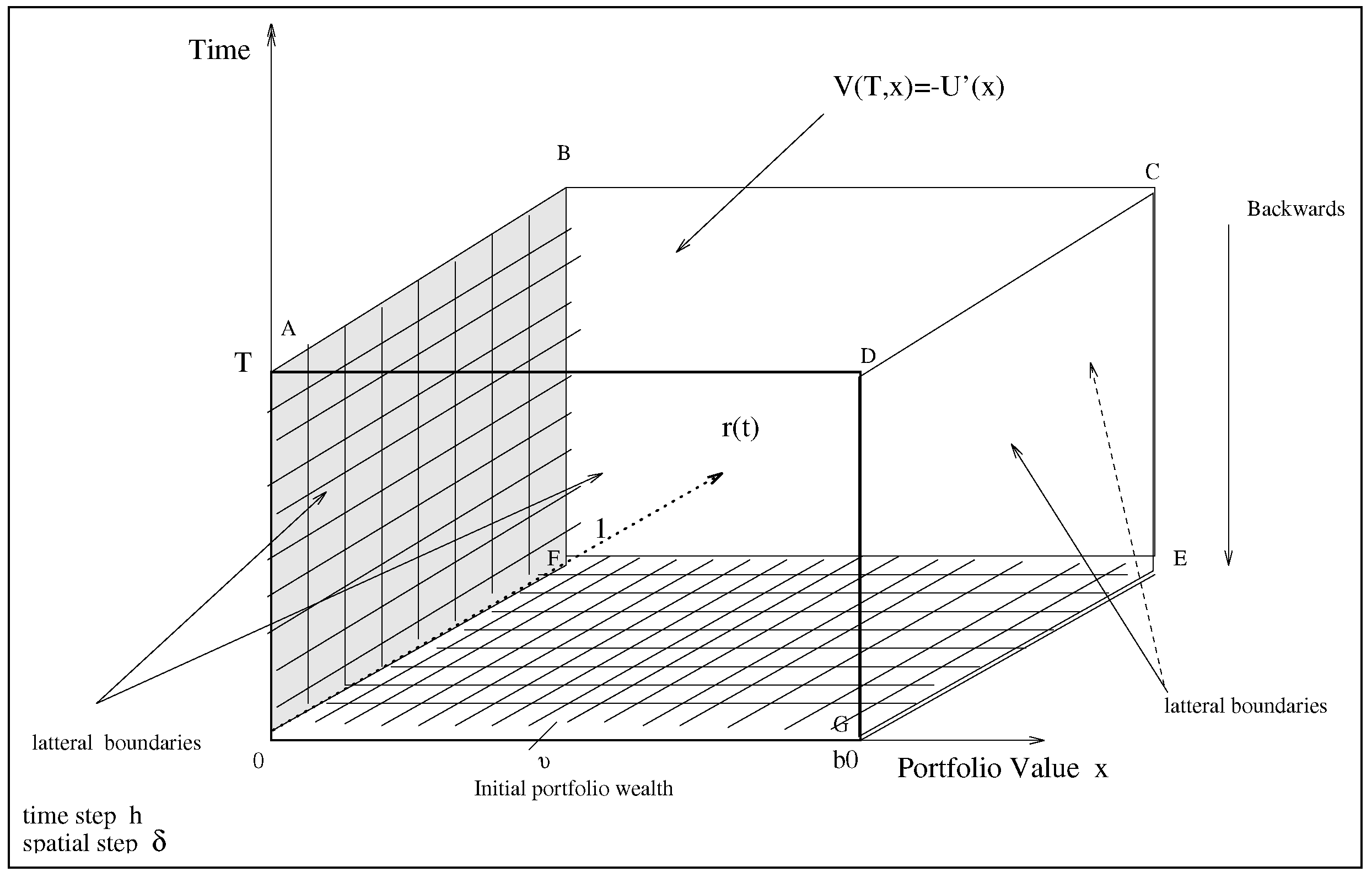
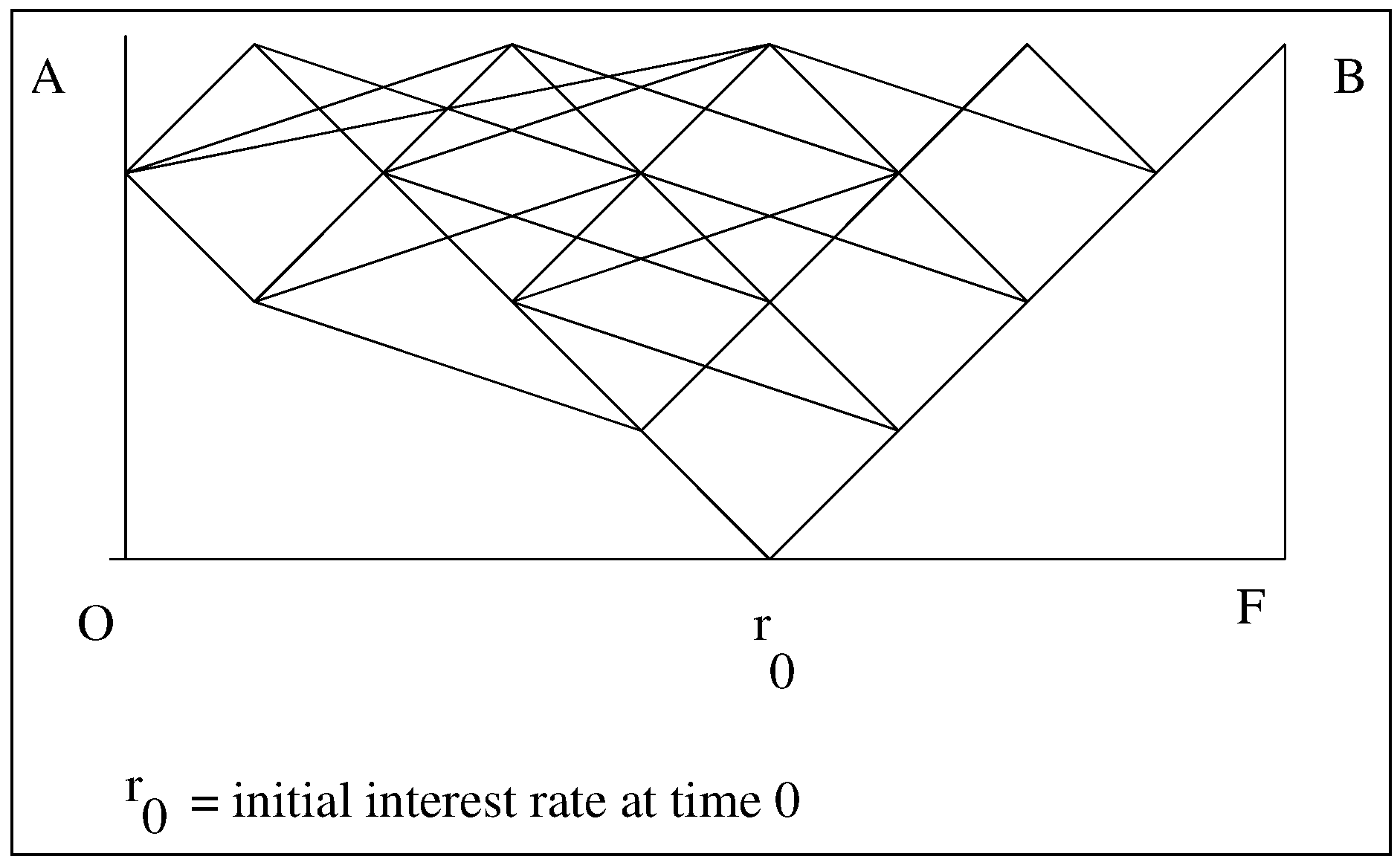
Since the f, a are non-linear with respect to the portfolio positions, and the control sets reflect, in essence, linear constraints on the portfolio positions, in order to apply the dynamic programming principle (8), we have to solve a non-linear problem at each point $(t,r(t),X(t\left)\right)$ progressing backwards in time. Thus, by referring to Figure 1 we have the following steps:

Step 1 

We first calculate the value of the derivatives and the portfolio sensitivities at each point $(t,r(t\left)\right)$ of the side $OABF$.

Step 2 

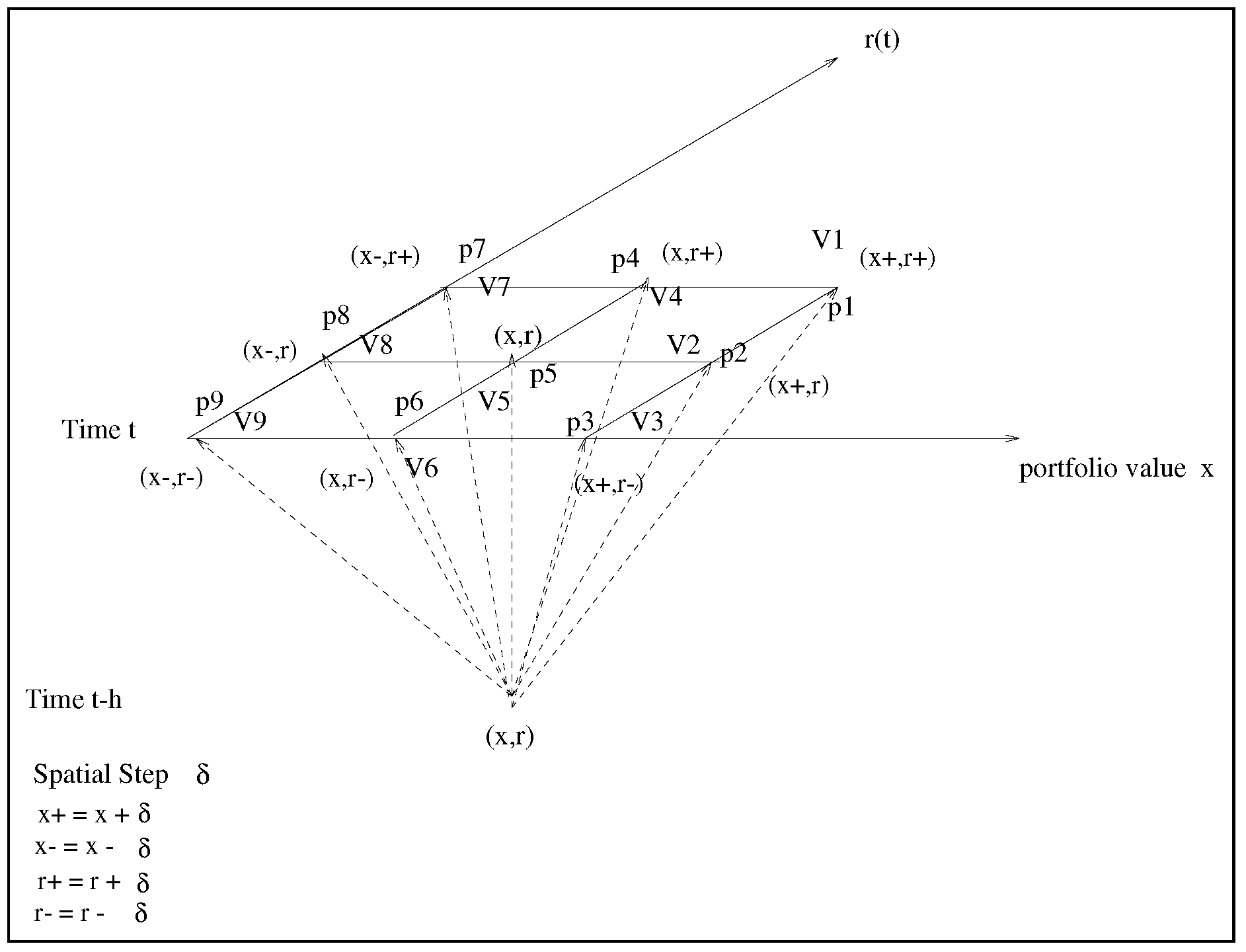
Since we know the value function over the sides $ABCD$, $OABF$, $DCEG$, $OADG$, we opt to calculate the value function starting from top to bottom (backwards in time). Taking a typical “slice” in time between $t-h$ and t (Figure 2), we see that the arrows starting from $(t-h,x,r)$ are the transition probabilities to time t. These are non-linear functions of the portfolio positions at time $t-h$, and their values are given according to equation (9). The value function at time $t-h$ and at state $(x,r)$ is given by the dynamic programming formula:

$$V(t-h,x,r)=\underset{\theta (t-h)\in U(t-h,x,r)}{min}\sum _{i=1}^9{p}_i{V}_i$$

(10)

where $p_i,i=1,\cdots ,9$ are the probabilities shown in the Figure 2, and $V_i$ are the values of the value functions at the nine points shown in the figure. This must be done for all the points $(x,r)$ at time $t-h$, before we move back to time $t-2h$. The whole procedure is repeated until we reach time zero. The optimization (10) is a non-convex problem. In fact the objective function is only continuous (it contains absolute values) and not differentiable. By introducing extra variables and transferring the absolute values to the set of algebraic constraints, we result in an optimization problem with quadratic constraints where standard convexification techniques can be applied ([29]).

Step 3 

For initial wealth v and for a particular level of the interest rate, we find the optimal portfolio positions that we adopt in order to meet our objectives. The whole evolution of the state dynamics can be found up to time T simply by following the tree created-by the state evolution probabilities. In addition, the procedure gives us, for every initial wealth and for every level of the interest rate, the evolution of the value function according to the state transition probabilities.

Figure 1. The Dynamic programming procedure.

Figure 1. The Dynamic programming procedure.

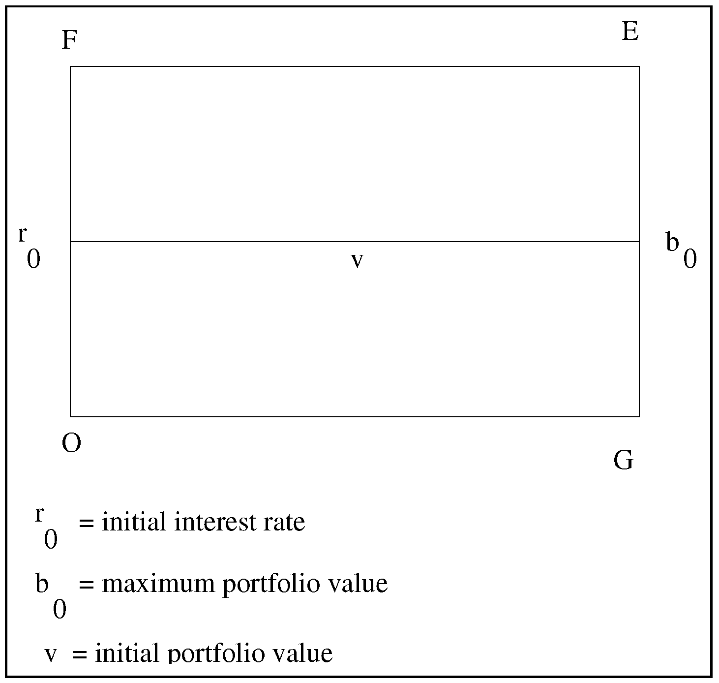
As it is shown in Figure 2, the portfolio value is very large in comparison with the interest rate r. In this case we rescale the portfolio axis, or we use different spatial steps ${\delta }_r,{\delta }_X$.

Figure 2. Time slice.

Figure 2. Time slice.

The method is adaptive by its nature and various adaptive estimation methods can be accommodated. In the case of a two factor model the whole analysis must be done in the Euclidean space ${\mathbb{R}}^4$. Various amendments of the method [28,30] can improve the speed and the convergence of the algorithm.

Figure 3. Embedding the tree structure into the stochastic control algorithm.

Figure 3. Embedding the tree structure into the stochastic control algorithm.

4.1. Numerical Implementation and Results

We have numerically implemented the above method using the generalised Hull and White model [21]. Based on this model we have valued all the derivatives of our portfolio. In order to optimize the algorithm and to reduce the number of non linear optimizations that have to be performed, we have embedded the recombining trinomial tree into the algorithm. This averts the need to employ the somewhat cumbersome numerical partial differential equation methods required for the valuation of the derivatives. In Figure 1, on the side $OABF$, the only relevant points are those of the embedded trinomial tree. In essence, the side $OABF$ is not a parallelogram any more, but a two-dimensional tree-structure (Figure 3). In order to reduce the number of non-linear optimizations, we opt not to solve the problem for all possible interest rate levels but only for the initial interest rate $r_0$. So at time 0 the optimization is performed only on the line $r_0{b}_0$ of the side $OFEG$ (Figure 4). The same happens in the previous steps, (i.e., the optimization is performed only for the relevant interest rate levels). In this way the algorithm becomes steadily faster as we move from time T to time 0. Since we know the maximum and minimum number of trading securities available for each time step, the maximum portfolio value per time step can be calculated and scaled analogously. In this way we further reduce the number of non-linear optimizations that have to be performed.

Figure 4. Optimization at time 0.

Figure 4. Optimization at time 0.

We present now a numerical example. The volatility of the short rate is assumed to be ${\sigma }_r(t,r\left(t\right))={\sigma }_r(0,r\left(0\right))r{\left(t\right)}^{\beta }$. The model characteristics are given in Table 2. The portfolio includes the following interest rate derivative securities: bonds, European and American calls on a bond, European and American puts on a bond, swaps, European and American payer’s swaptions, European and American receiver’s swaptions, caps and floors. 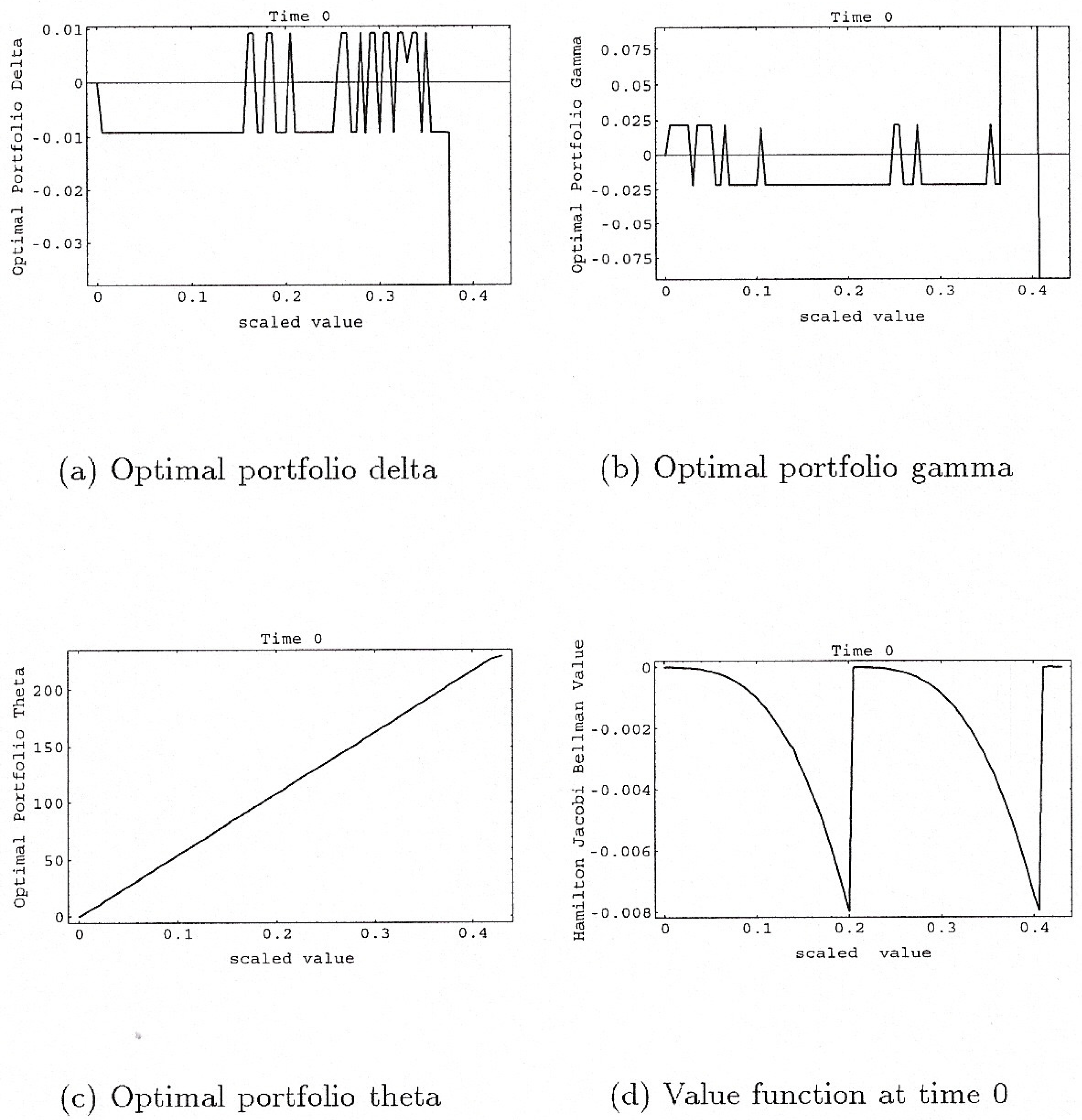Their characteristics are presented in Table 1. Deltas and gammas of the derivatives are calculated with respect to the bond. Naturally the delta of the bond is 1 and the gamma is 0. The portfolio theta is calculated as the local expected portfolio growth per time period. That is why we observe the linear relationship between optimal portfolio theta and optimal portfolio value Figure 5c. We feel that this definition of theta is more suitable to practical applications. Of course the classical portfolio theta definition could have been applied as well. For reasons of simplicity we do not have a cash account. We assume that the utility function is $U^{\prime }\left(x\right)=x^3$ and the portfolio optimization horizon is 7 time steps $(7\Delta t)$. For scaling purposes we assume that the number of available derivative securities is any number in the interval $[-10,10]$. This constraint can be relaxed so that at each time step (or even at each state as well) it is feasible to have different maximum and minimum levels of available derivatives. We impose the risk limits given in Table 3 for every time step.

Table 1. Derivative Characteristics.

bond		swap
Starting Period	0	Starting Period	0
Maturity Period	19	Maturity Period	19
Coupon Period	2	Coupon Period	2
Coupon Rate	0.10	Coupon Rate	0.10
Principal	100.0	Notional Principal	100.
European bond call		European bond put
Starting Period	0	Starting Period	0
Maturity Period	10	Maturity Period	10
Exercise Price	80.5	Exercise Price	80.5
Bond Staring Period	0	Bond Staring Period	0
Bond Maturity Period	19	Bond Maturity Period	19
Bond Coupon Period	2	Bond Coupon Period	2
Bond Coupon Rate	0.1	Bond Coupon Rate	0.1
Bond Principal	100	Bond Principal	100
American bond call		American bond put
Starting Period	0	Starting Period	0
Maturity Period	10	Maturity Period	10
Exercise Price	80.5	Exercise Price	80.5
Bond Staring Period	0	Bond Staring Period	0
Bond Maturity Period	19	Bond Maturity Period	19
Bond Coupon Period	2	Bond Coupon Period	2
Bond Coupon Rate	0.1	Bond Coupon Rate	0.1
Bond Principal	100	Bond Principal	100
European receiver’s Swaoption		European payer’s put
Starting Period	0	Starting Period	0
Maturity Period	10	Maturity Period	10
Exercise Price	6.5	Exercise Price	80.5
Swap Staring Period	0	Bond Maturity Period	0
Swap Maturity Period	19	Bond Staring Period	19
Swap Reset Period	2	Bond Coupon Period	2
Swap Fixed Rate	0.1	Bond Coupon Rate	0.1
Swap Notional Principal	100	Bond Principal	100
American receiver’s Swaoption		American payer’s put
Starting Period	0	Starting Period	0
Maturity Period	10	Maturity Period	10
Exercise Price	6.5	Exercise Price	80.5
Swap Staring Period	0	Bond Staring Period	0
Swap Maturity Period	19	Bond Maturity Period	19
Swap Reset Period	2	Bond Coupon Period	2
Swap Fixed Rate	0.1	Bond Coupon Rate	0.1
Swap Notional Principal	100	Bond Principal	100
cap		floor
Starting Period	0	Starting Period	0
Maturity Period	10	Maturity Period	10
Reset Period	2	Reset Period	2
Cap rate	0.1	Floor rate	0.1
Cap Notional Principal	100	Floor Notional Principal	100

Table 1. Derivative Characteristics.

bond		swap
Starting Period	0	Starting Period	0
Maturity Period	19	Maturity Period	19
Coupon Period	2	Coupon Period	2
Coupon Rate	0.10	Coupon Rate	0.10
Principal	100.0	Notional Principal	100.
European bond call		European bond put
Starting Period	0	Starting Period	0
Maturity Period	10	Maturity Period	10
Exercise Price	80.5	Exercise Price	80.5
Bond Staring Period	0	Bond Staring Period	0
Bond Maturity Period	19	Bond Maturity Period	19
Bond Coupon Period	2	Bond Coupon Period	2
Bond Coupon Rate	0.1	Bond Coupon Rate	0.1
Bond Principal	100	Bond Principal	100
American bond call		American bond put
Starting Period	0	Starting Period	0
Maturity Period	10	Maturity Period	10
Exercise Price	80.5	Exercise Price	80.5
Bond Staring Period	0	Bond Staring Period	0
Bond Maturity Period	19	Bond Maturity Period	19
Bond Coupon Period	2	Bond Coupon Period	2
Bond Coupon Rate	0.1	Bond Coupon Rate	0.1
Bond Principal	100	Bond Principal	100
European receiver’s Swaoption		European payer’s put
Starting Period	0	Starting Period	0
Maturity Period	10	Maturity Period	10
Exercise Price	6.5	Exercise Price	80.5
Swap Staring Period	0	Bond Maturity Period	0
Swap Maturity Period	19	Bond Staring Period	19
Swap Reset Period	2	Bond Coupon Period	2
Swap Fixed Rate	0.1	Bond Coupon Rate	0.1
Swap Notional Principal	100	Bond Principal	100
American receiver’s Swaoption		American payer’s put
Starting Period	0	Starting Period	0
Maturity Period	10	Maturity Period	10
Exercise Price	6.5	Exercise Price	80.5
Swap Staring Period	0	Bond Staring Period	0
Swap Maturity Period	19	Bond Maturity Period	19
Swap Reset Period	2	Bond Coupon Period	2
Swap Fixed Rate	0.1	Bond Coupon Rate	0.1
Swap Notional Principal	100	Bond Principal	100
cap		floor
Starting Period	0	Starting Period	0
Maturity Period	10	Maturity Period	10
Reset Period	2	Reset Period	2
Cap rate	0.1	Floor rate	0.1
Cap Notional Principal	100	Floor Notional Principal	100

The number of non linear optimization problems of the form (10) that have been solved is 5237. The value function at time 0 is depicted in Figure 5d. As we can see it is negative, something that it is expected since our objective is the minimisation of minus the utility function of terminal wealth.

Table 2. Yield curve characteristics.

Declining Initial Term Structure and Initial Volatility Structure
Time Horizon $\left(N\right)$	20
Time Step $(\Delta t)$	1
β	1
Initial Volatility $\left(V\right(0\left)\right)$	0.14
Initial Term Structure at time $i\Delta t$	$0.1(1+(i\Delta t)/70)$
Initial Volatility Structure at at time $i\Delta t$	$0.14(1+(i\Delta t)/110)$

Table 2. Yield curve characteristics.

Declining Initial Term Structure and Initial Volatility Structure
Time Horizon $\left(N\right)$	20
Time Step $(\Delta t)$	1
β	1
Initial Volatility $\left(V\right(0\left)\right)$	0.14
Initial Term Structure at time $i\Delta t$	$0.1(1+(i\Delta t)/70)$
Initial Volatility Structure at at time $i\Delta t$	$0.14(1+(i\Delta t)/110)$

Figure 5. Optimal Portfolio sensitivities and value function at time 0.

Figure 5. Optimal Portfolio sensitivities and value function at time 0.

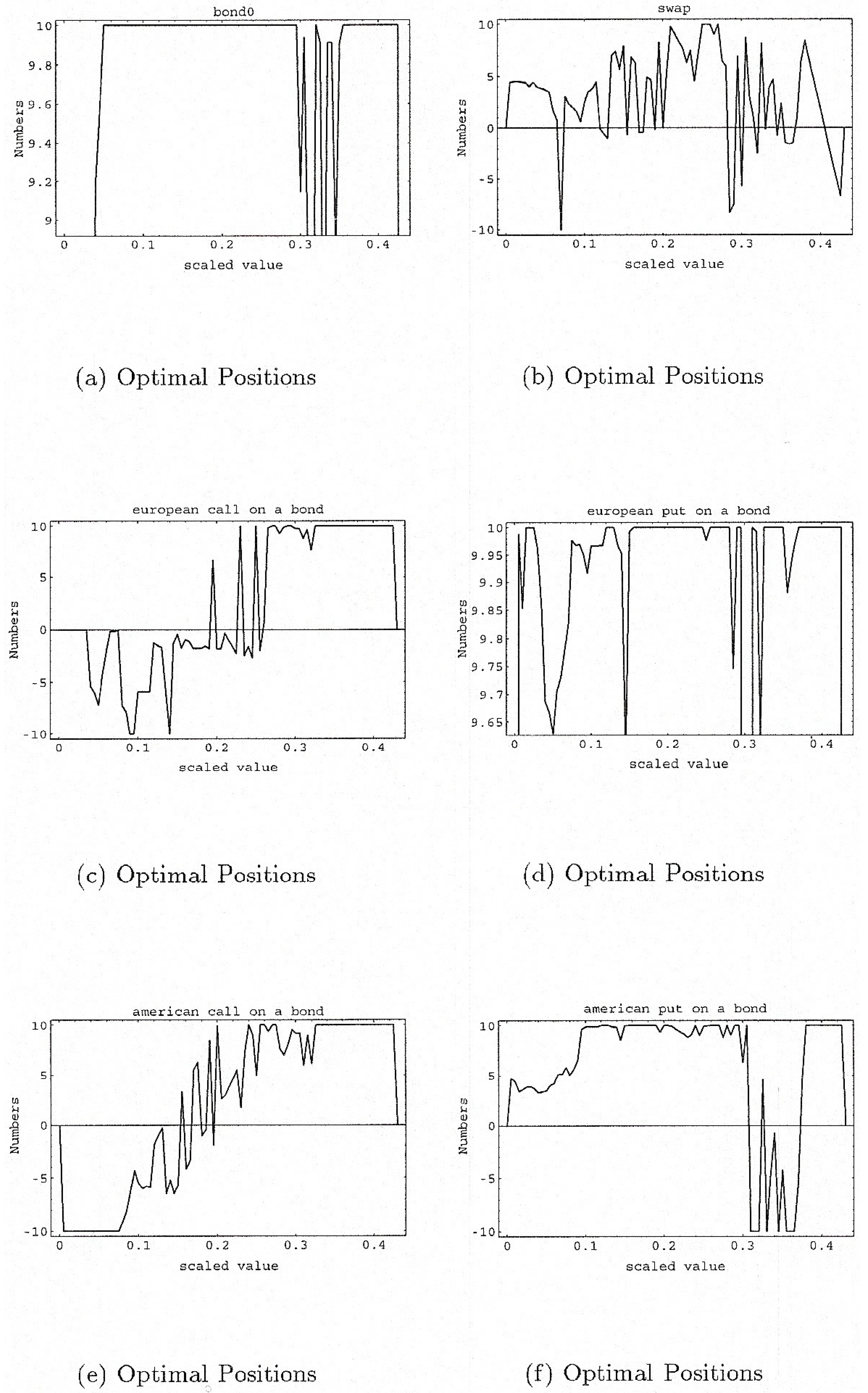
Figure 6. Optimal Positions at time 0.

Figure 6. Optimal Positions at time 0.

Figure 7. Optimal Positions at time 0.

Figure 7. Optimal Positions at time 0.

Table 3. Portfolio risk profile.

Risk Limits
Delta limit $\left(\delta \right)$	0.009211
Gamma limit $\left(\gamma \right)$	0.021584
Theta limit $\left(\theta \right)$	1.696839

Table 3. Portfolio risk profile.

Risk Limits
Delta limit $\left(\delta \right)$	0.009211
Gamma limit $\left(\gamma \right)$	0.021584
Theta limit $\left(\theta \right)$	1.696839

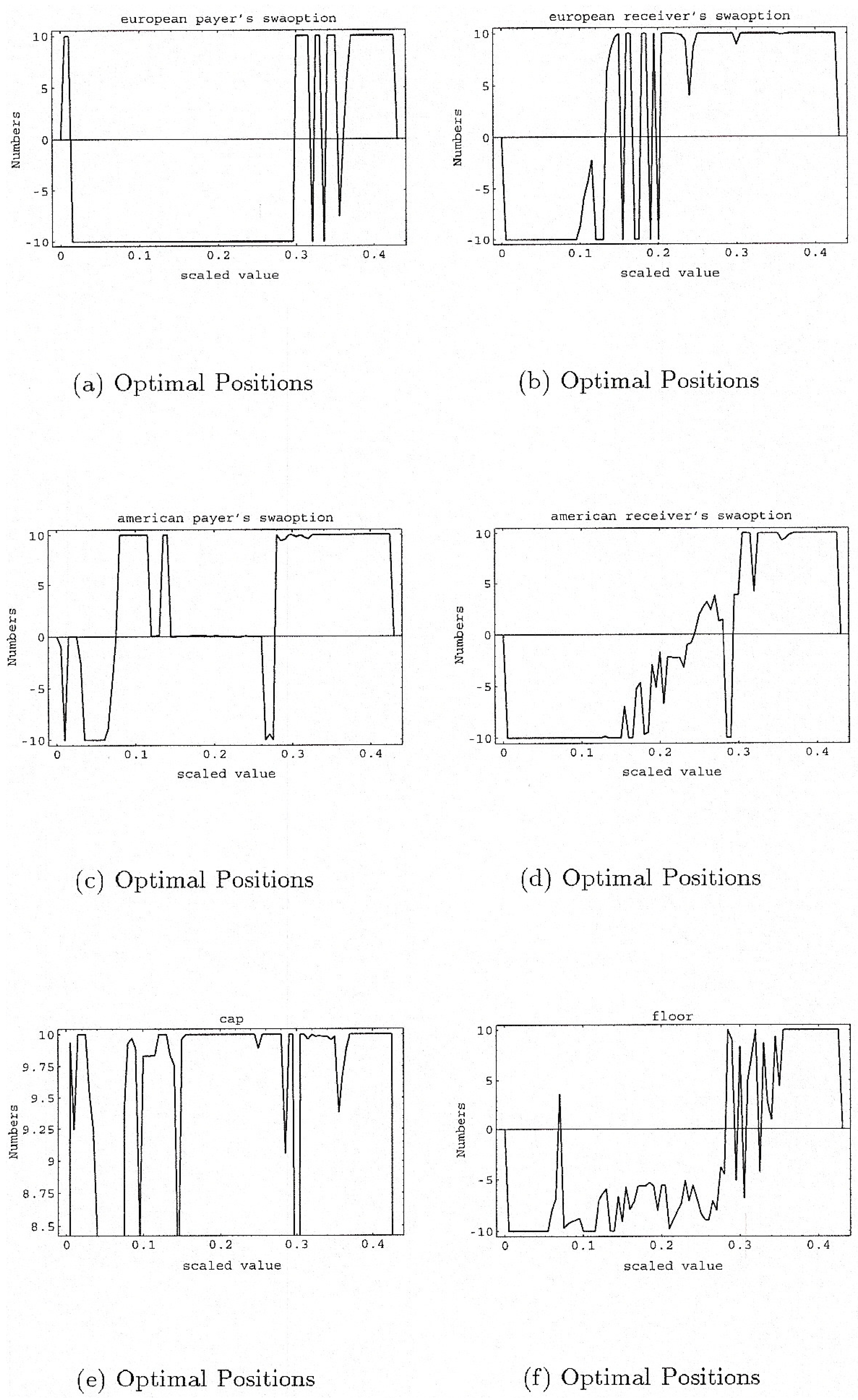
Optimal portfolio positions at time zero are given in Figure 6 and Figure 7. Figures 5a–c show the sensitivities of the optimal portfolio at time 0, all within the boundaries defined in Table 3. Moreover, we see that the optimal portfolio is exposed often to the maximum permitted level of risk(graphics for the optimal portfolio positions, optimal portfolio delta, gamma, theta and for the Hamilton-Jacobi-Bellman equation for the times $i\Delta t,i=1,2,3,4,5,6,7$ are available from the authors upon request). By design the algorithm is eager to construct portfolios with the maximum permitted level of risk as expressed in Table 3. This is natural since the risk limits are the maximum allowable limits that can be taken in order to achieve the maximum possible portfolio value, given risk preferences, that are expressed through the utility function.

5. Conclusions

In this paper, we address the risk management control problem of derivatives in the interest rate market. By formulating the problem as a stochastic portfolio optimization one with constraints, techniques from the stochastic control theory can be used so that the financial institution meets the various objectives being set internally or externally, through the control of the evolution of portfolio positions. The main advantage of this approach is that we do not have to assume anything about the utility function except for continuity. From our computer implementation, we have observed that the method is sensitive to different initial values (initial term structure and volatility structure) and different boundary conditions (utility functions). Finally we note the flexibility of the proposed discretization scheme. As in Section 4, the probabilities do not have to be of the form (7). The locally approximating Markov chain is not unique. There is freedom for the choice of the chain in order to improve the convergence of the algorithm.

The method quantifies the risk return characteristics of the derivatives portfolio through portfolio sensitivities in a specific way by allowing the creation of optimal portfolios with desired risk/return characteristics. The fact that control sets can be time and state dependent gives us a great flexibility in incorporating limits in case of tail risks. Incorporation of VAR or CVAR limits (possibly time and state dependent) as additional constraints in the control sets are possible.

In light of the recent financial crisis where unwanted or miscalculated risks in the derivatives area caused many financial institutions to go bankrupt and endangered the whole economy by triggering systemic risks, this type of approach, that gives emphasis on the on-line monitoring and control of derivatives portfolio, could be useful in the future either to avoid similar situations or at least to mitigate their consequences.