1. INTRODUCTION
Most research on understanding the behavior of stock prices is based on the present value model (PVM) or the more general consumption-based model. The present value model was rejected in the early 1980s by LeRoy and Porter (1981), Shiller (1981), and West (1988) when applied to real economic data. The consumption-based model, which allows for a stochastic discount factor, was also found unable to fully support both the level and volatility of stock prices by an extensive literature originating with the work of Mehra and Prescott (1985).
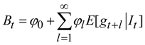
Several modifications of the two models as well as alternatives have been suggested. For instance, more precise measures of fundamentals such as broad dividends and net payouts in place of traditional cash dividends in the present value model, habit formation in consumption designed to add volatility to the stochastic discount factor in the consumption-based model to overcome smoothness in observed consumption, new utility functions such as Epstein-Zin (1989) recursive utility, heterogeneous agent models, irrational expectations on the part of investors, and bubbles have been proposed to resolve the discrepancy between the empirical implications of the two models and observed stock market data. However, none of these explanations has been convincing enough to stop the search for alternative explanations for rationalizing movements in stock prices.
The impetus to this paper is that macroeconomic factors such as business cycle indicators are found to have predictive power over stock market returns. If we incorporate these macroeconomic factors (as non-fundamentals), these factors along with fundamentals may be able to explain stock prices better.
It is well known that stock prices are procyclical. Broad dividends, net payouts, or other forms of fundamentals do not show this pattern. The present value model with a constant discount rate cannot explain this comovement of stock prices with business cycles. Also, inherent smoothness in observed consumption determining the stochastic discount factor in the consumption-based model does not provide enough volatility around business cycles to explain this procyclical pattern of stock prices either. Other alternatives to the two models noted earlier are not able to address this property as well.
Stock markets have never been isolated from other economic activity. As Fischer and Merton (1984) state, there is a close empirical connection between stock market movements and the subsequent behavior of the economy. The consumption-based model of Lucas (1978) is the simplest general equilibrium asset pricing model. It relates stock prices to the real economy by equating the stochastic discount factor to the intertemporal marginal rate of substitution which is a function of aggregate optimal consumption.
But, considering the quite smooth consumption data since World War II, the high returns and volatility of stock returns have been perplexing. Unless risk aversion is much higher than is deemed acceptable, these equity premium and excess volatility puzzles (see Mehra and Prescott (1985) and Shiller (1981)) cannot be resolved.
Lately, many economists have tried to use macroeconomic factors to predict asset returns since, apparently, information drawn from the past values of dividends and aggregate consumption alone is not sufficient to understand movements in stock prices. These macro factors contain independent information, besides the fundamentals, to account for the procyclical pattern of stock prices.
In this study, we try to address whether stock prices, fundamentals, and non- fundamentals are cointegrated. A theory free Vector Autoregression (VAR) framework developed from the consumption-based model is used to test for cointegration between these three variables. Cointegration between them would suggest that stock prices share a common long run linear trend with fundamentals and macro factors. If we cannot find cointegration between them, there may be either a nonlinear relationsip between these variables or we may have missed some other elements, such as expectations generated from new technologies.
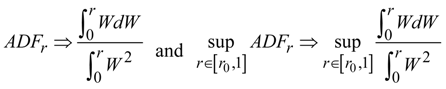
But, even if we find cointegration between stock prices, fundamentals, and macro factors, it still does not rule out the presence of periodically collapsing bubbles (as described in Evans (1991)). These could potentially make the behavior of an explosive series appear like an I(1) or even stationary series. Phillips et al. (2007) discuss this issue. They develop ADFr and sup ADFr statistics to test for the existence of periodically collapsing bubbles.
The rest of the paper is organized as follows.
Section 1 discusses literature related to the measures of fundamentals and macro factors (non-fundamentals) used in the paper.
Section 2 builds up the theoretical model.
Section 3 develops the VAR framework as well as the single equation model for cointegration tests, and discusses the sup augmented test for periodically collapsing bubbles.
Section 4 describes the data and provides empirical results of the analysis.
Section 5 concludes with a summary of the main findings of the paper. An appendix provides technical details on the sup augmented test for periodically collapsing bubbles.
2. RELATED LITERATURE
2.1. Fundamentals (Broad Dividends)
Traditional cash dividends have failed to satisfy the Euler equation of the consumption- based asset pricing model of Lucas (1978) since the 1980s. Modern dividend policy has distorted investors’ judgments on the true profitability of a firm. Fama and French (2001) address the disappearing dividends phenomenon. Boudoukh et al. (2007) show that repurchases had substituted for dividends over the last 20 years since SEC rule 10b-18 was released in 1985, which provided a legal safe harbor for firms to repurchase shares. A structural break is found in dividend yield series around the time of the enactment of this rule. New measures of dividends are therefore useful.
Boudoukh et al. (2007) find total payouts and net total payouts to have significant predictive power for equity returns instead of narrow dividends. Total payouts are the sum of narrow dividends and repurchases. Net total payouts are total payouts less seasoned equity issues. These payouts refer to distributed cash flows going to shareholders. No instability is detected in these payout measures around the time of release of the SEC rule 10b-18.
Regression of returns on the payout yield over the period 1926 to 1985 show that payout yield coefficient is very similar to that found in the period 1926 to 2003, which shows that repurchases have substituted for dividends over the later period. At the same time, net total payout yield shows a striking explanatory power for excess market returns compared with dividend yield and total payout yield. The results in Boudoukh et al. (2007) imply that asset pricing tests employing measures of cash distributions to shareholders are less likely to accurately capture effects of fundamentals if these studies ignore repurchases.
Broad dividends include not only conventional cash dividends but also other forms of cash payouts to shareholders (e.g., share repurchases and acquisitions). So, they still apply to firms for which regular cash dividends are 0. Broad dividends are valid for companies which substitute dividends with repurchases, and companies which have earnings but postpone payments of dividends until much later in their life cycle.
Broad dividends are chosen in this study to replace narrow traditional dividends as fundamentals. Broad dividends Xt are calculated as earnings Rt in time period t minus all changes in book value (Bt − Bt−1) , Xt = Bt−1 + Rt − Bt. See Ohlson (1991, 1995), Feltham and Ohlson (1995), and Jiang and Lee (2005) for a detailed discussion of broad dividends and related cash flow measures.
While broad dividends include more information than net total payouts, such as acquisitions and any other changes in book values, it is not clear that those acquisitions, along with some repurchases, would be taken as information when forming expectations of future payouts. Also, for companies who do not have much earnings and do not pay much dividends but have high values, such as dot com companies in early stages in their life cycle, broad dividends do not have much theoretical explanatory power. Predicting future payouts of such companies requires more information than that contained in just the historical data, such as for instance the age of companies explored in Pastor and Veronesi (2003). But, in this paper, we take a simpler approach and view such information as noise outside of the investors’ information set.
2.2. Non-Fundamentals (Macroeconomic Factors)
Lee (1998), Allen and Yang (2000) use a Trivariate Moving Average (TMA) to model how prices behave in response to three types of innovations: permanent and temporary changes in fundamentals, and non-fundamental factors, by imposing restrictions on the model to identify each kind of innovations. Results show that non-fundamentals contribute a substantial fraction to the variance of the Australian stock market data. But they do not specify what the non-fundamental factors are nor their characteristics.
Ludvigson and Ng (2005) perform dynamic factor analysis with large datasets to investigate possible empirical linkages between forecastable variation in excess returns of one through five year zero coupon U.S. Treasury Bond and macroeconomic fundamentals. Several common factors generated from large datasets of 132 economic series have strong explanatory power for excess returns. Rangvid (2006) shows that the ratio of share prices to GDP tracks a larger fraction of variation over time in expected returns on the aggregate stock market than do price-earnings and price-dividend ratios.
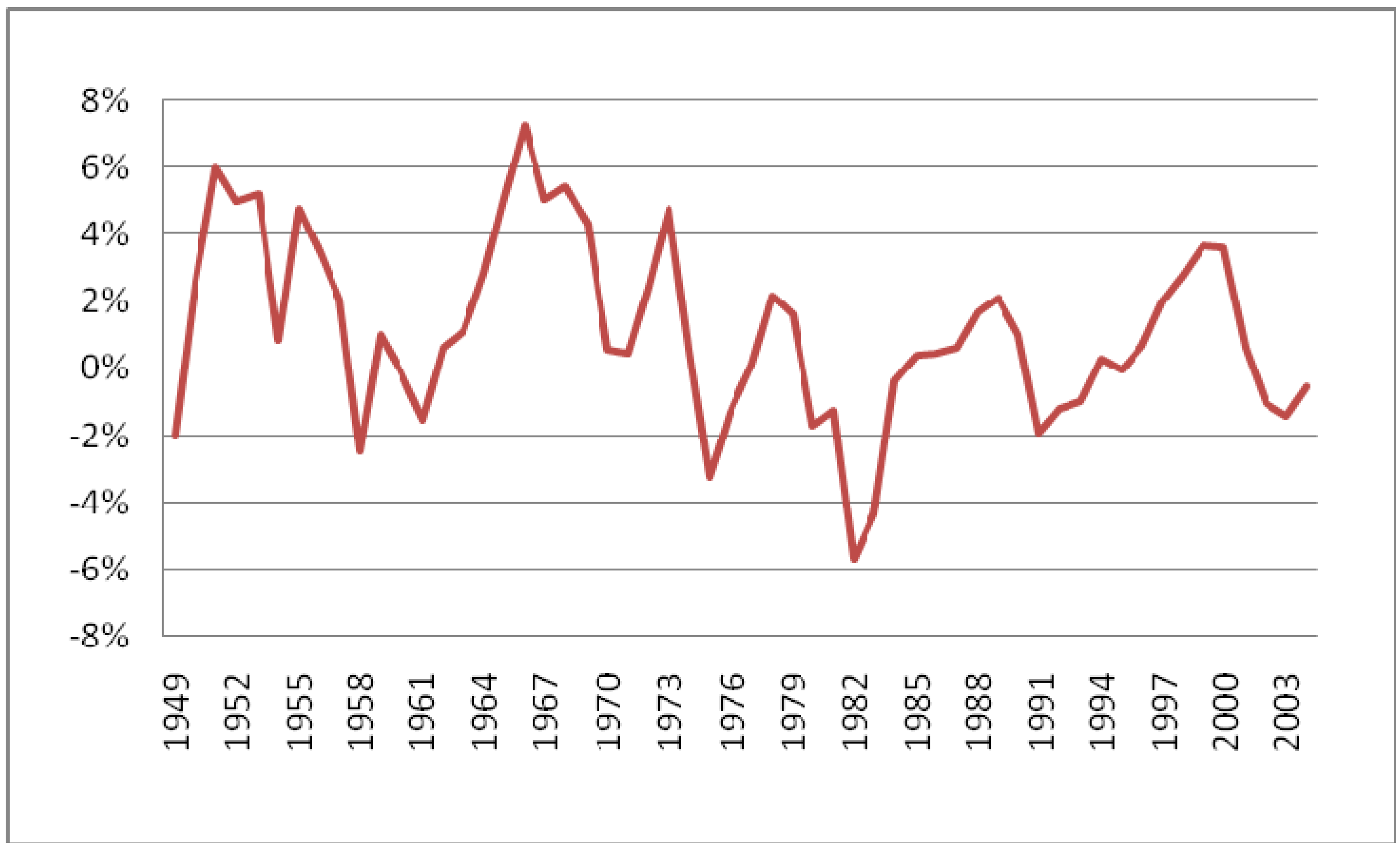
Cooper and Priestley (2007) single out the output gap, a production based macroeconomic variable and prime business indicator, as the non-fundamental factor. Their work shows that output gap is a strong predictor of U.S. stock returns and that it forecasts returns both in- and out-of-sample. As discussed in Cooper and Priestley (2007), the output gap has several apriori advantages over other predictive variables, including price ratios such as Lettau and Ludvigson’s (2001) cay. Moreover, as noted in Cochrane (2005), the output gap uses only production-related data and, hence, its predictive power constitutes independent evidence regarding the variation of risk premia over the business cycle.
Thus, the above studies have shown that non-fundamental factors are important for explaining stock price fluctuations. Moreover, we can specify the output gap as one such factor. But they do not address whether this factor is sufficient to explain the volatility of stock prices.
Most research, including all the studies mentioned above, explore only a linear relationship between stock prices and macro factors correlations between returns and the macro factors.
5. EMPIRICAL RESULTS
5.1. Data
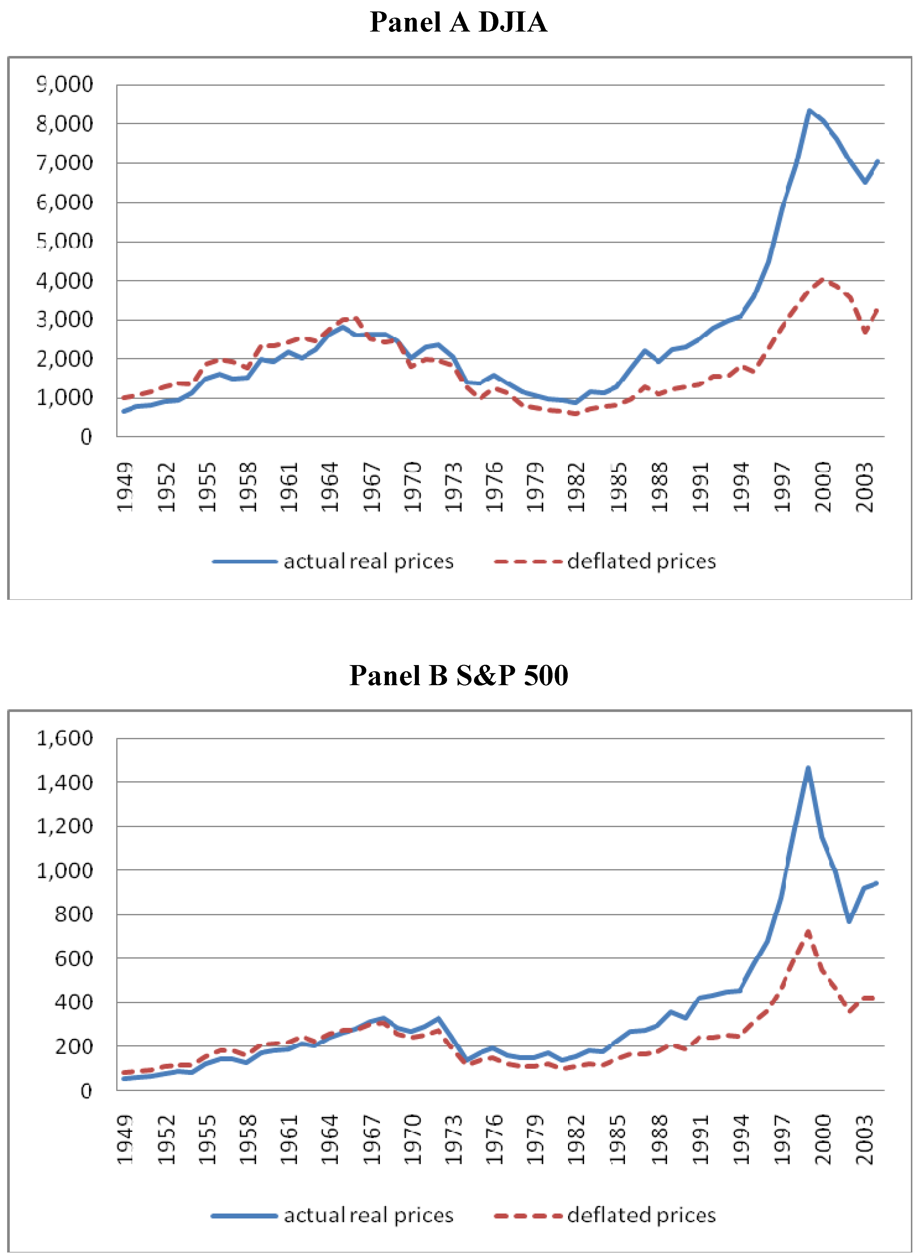
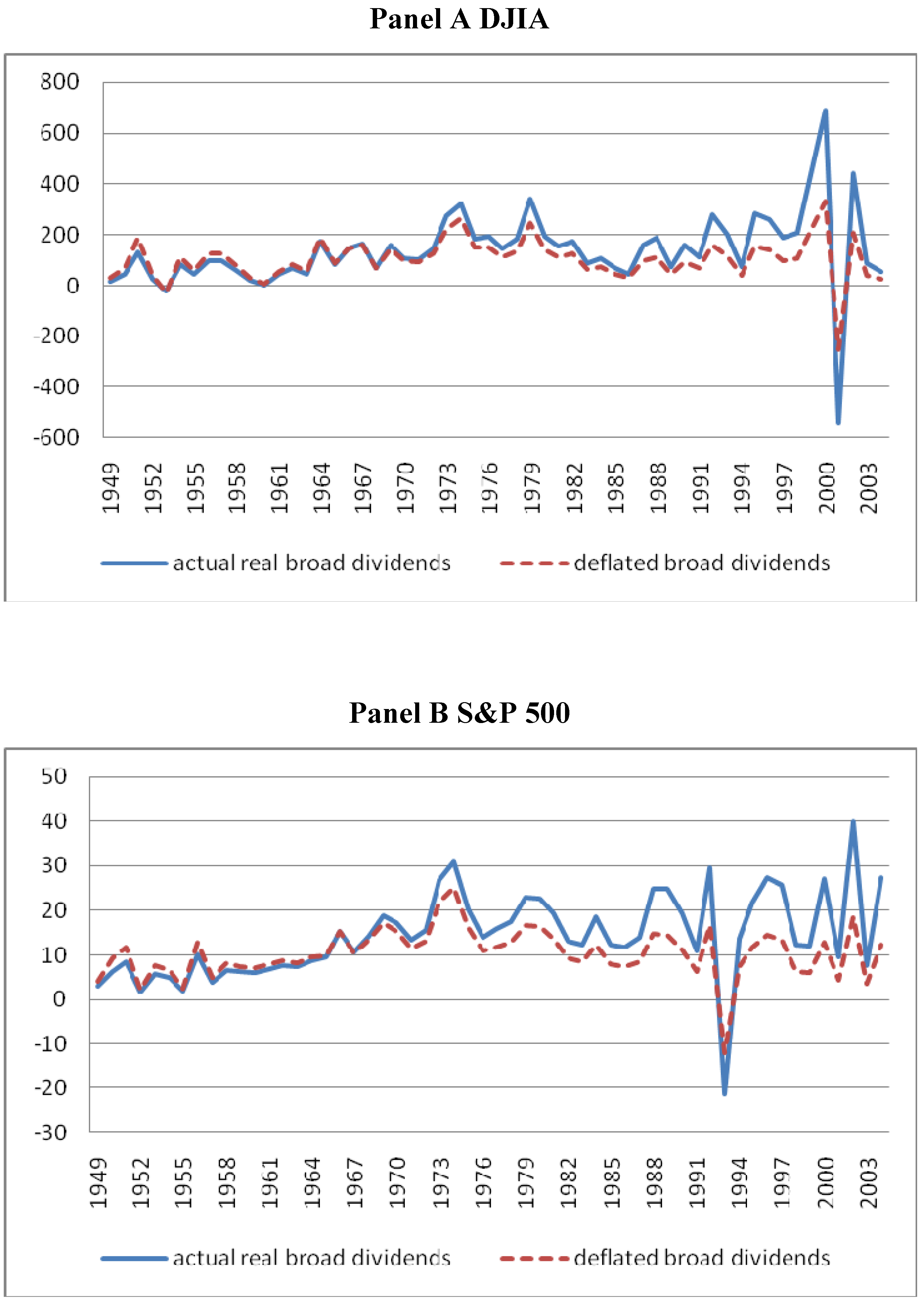
We use two data sets, Standard and Poor 500 (S&P 500) and Dow Jones Industrial Average (DJIA) indices. Both contain annual aggregate price indices, earnings, and book values from 1949-2004. Annual prices are calculated as prices in January divided by producer price index (PPI). Earnings and book values are also deflated by the PPI. Index earnings series are earnings per share, adjusted to index, 4-quarter total, fourth quarter. S&P index data is obtained from CRSP, and annual DJIA index data are from Value Line publication, A Long-Term Perspective: Dow Jones Industrial Average. Seasonally adjusted observations on aggregate real consumption of nondurables and services are obtained from Federal Reserve Board publications. Real per capita consumption series are constructed by dividing each observation by population, published by the Bureau of Census. Output gap is obtained from St. Louis Fed Economic Data.
It is well-known that, in order to explain the equity premium puzzle, the CRRA coefficient α needs to be much higher than a value of one. West (1988) shows that α needs to take a value higher than 1 in order to meet the volatility test of the consumption- based model. Here, we choose a reasonably low number for α to avoid the suspicion that a high value for α is what accounts for movements in stock prices that we are interested in understanding. A value of 1.001 is assigned, although alternatively choosing a value of 0.99, 1, or 1.05 for would not materially affect our conclusions.
5.2. Results
5.2.1. Tests for Unit Roots
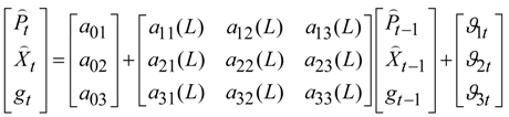
A preliminary test is done to check for unit roots in variables appearing in the TVAR model of Equation (12). An augmented Dickey-Fuller (ADF) test is performed on stock prices Pt, broad dividends Xt, and the output gap gt. We also test raw (not deflated by marginal utility) stock prices Pt and broad dividends Xt for comparison.
Table 1 reports the ADF test statistics. All statistics are larger than the left tail critical values at the 0.05 significance level. Thus, we fail to reject a unit root in all the variables.
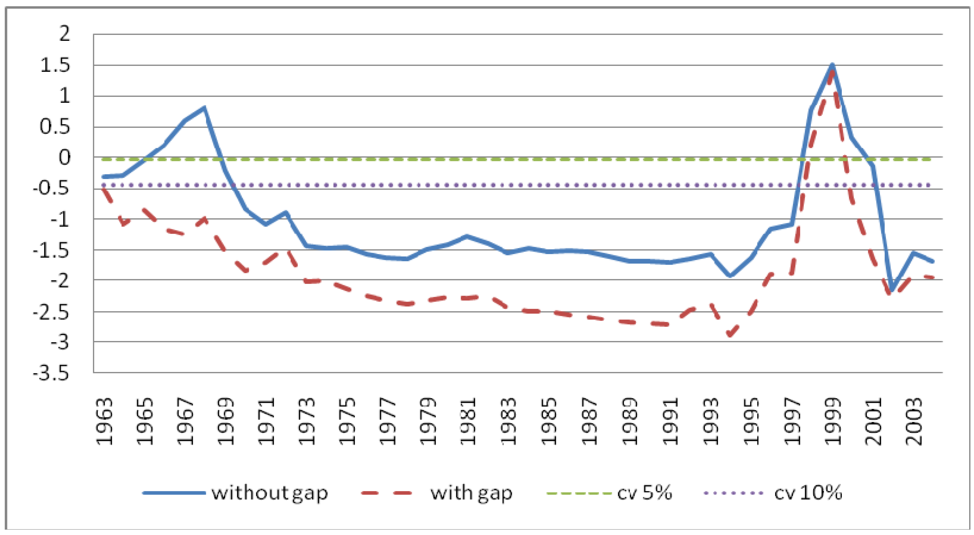
We next check correlation between the output gap and each of stock prices and dividends.
Table 2 provides the coefficient of determination in individual regressions of
Xt,
,
Pt,
on
gt, respectively. Their pairwise correlation coefficient is also reported in the table. We find that broad dividends, whether deflated by marginal utility or not, have no significant correlation with
gt, since values of the coefficient of determination and the correlation coefficient are both very low. This indicates that the output gap contains information that is orthogonal to broad dividends.
Raw (not deflated by marginal utility) stock prices Pt also show low correlation with the output gap. However, stock prices deflated by marginal utility show higher correlation, as high as 0.35 for DJIA data.
5.2.2. Tests for Cointegration
We now proceed to test for cointegration between stock prices, broad dividends, and the output gap using the TVAR and single equation frameworks of
section 3.1 and
section 3.2. For comparison of results with the TVAR framework, a bivariate Vector Autoregression (BVAR) model of broad dividends and stock prices is also tested. Unlike the BVAR framework of Campbell and Shiller (1986), our BVAR model is unrestricted for ease of comparison with the TVAR framework.
The cointegration tests used here follow the procedures of Johansen (1988) and Stock and Watson (1988). See Enders (1995) for a textbook exposition. Results are reported in
Table 3,
Table 4,
Table 5 and
Table 6.
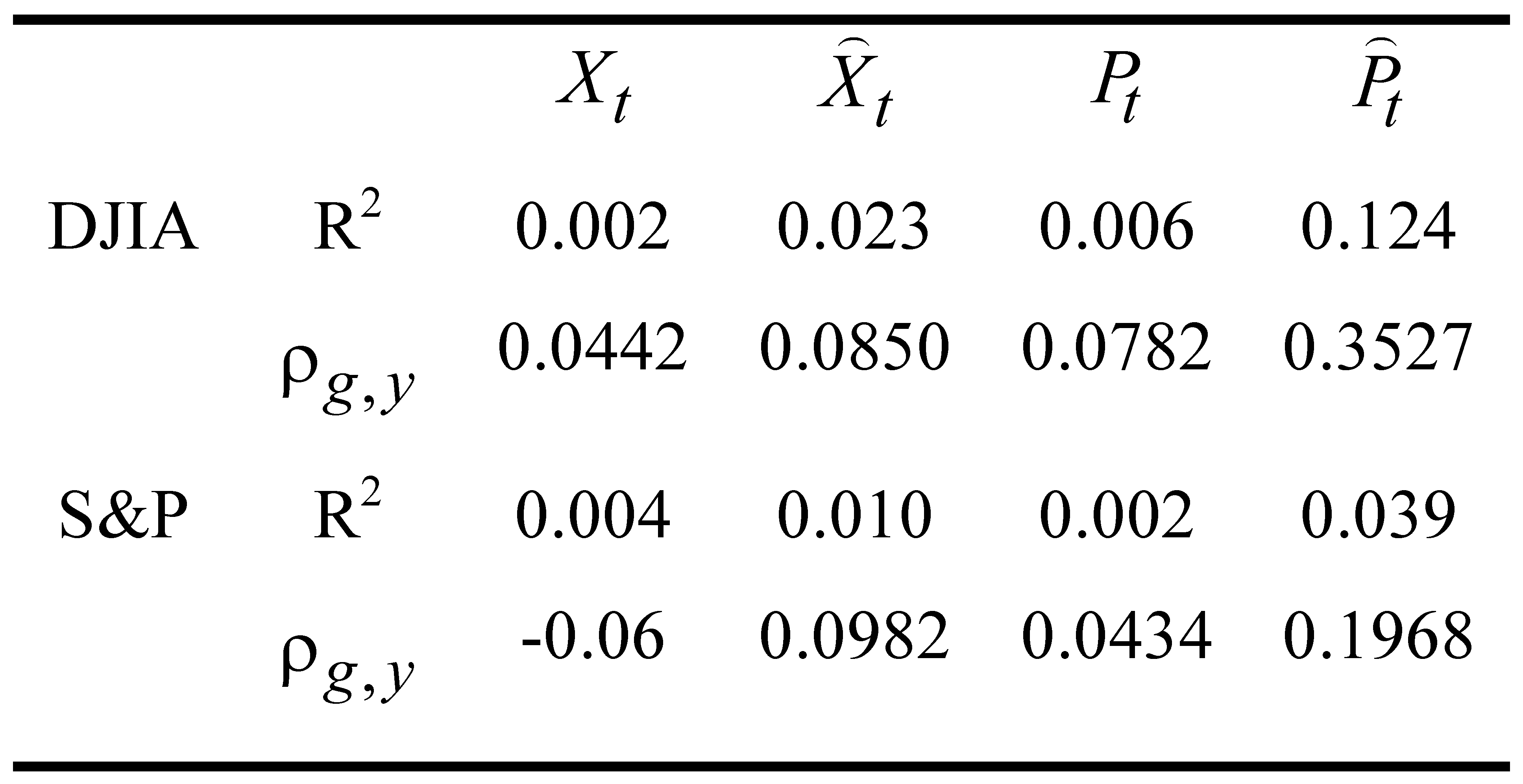
r is the number of linearly independent cointegrating vectors. The null hypothesis stated in the first column
r ≤
x is that there are
x or less than
xindependent cointegrating vectors against the alternative
r=
x+1,
x+ 2,...,
or n, where
n is the length of the vector being tested for cointegration (2 for BVAR models and 3 for TVAR models). If the test statistic is larger than critical value, we reject the null hypothesis.
In what follows, we make three comparisons of test results. First, we compare test results from the BVAR and the TVAR frameworks (Panels A versus B in
Table 3,
Table 4,
Table 5 and
Table 6). Second, we compare results for raw stock prices and dividends not deflated
by marginal utility (that is,
Table 3 and
Table 4 labeled ‘without consumption data’) with the deflated versions of these variables (that is,
Table 5 and
Table 6 labeled ‘with consumption data’). Third, we compare results of DJIA data with S&P 500 data (that is, compare
Table 3 versus 4, and
Table 5 versus 6).
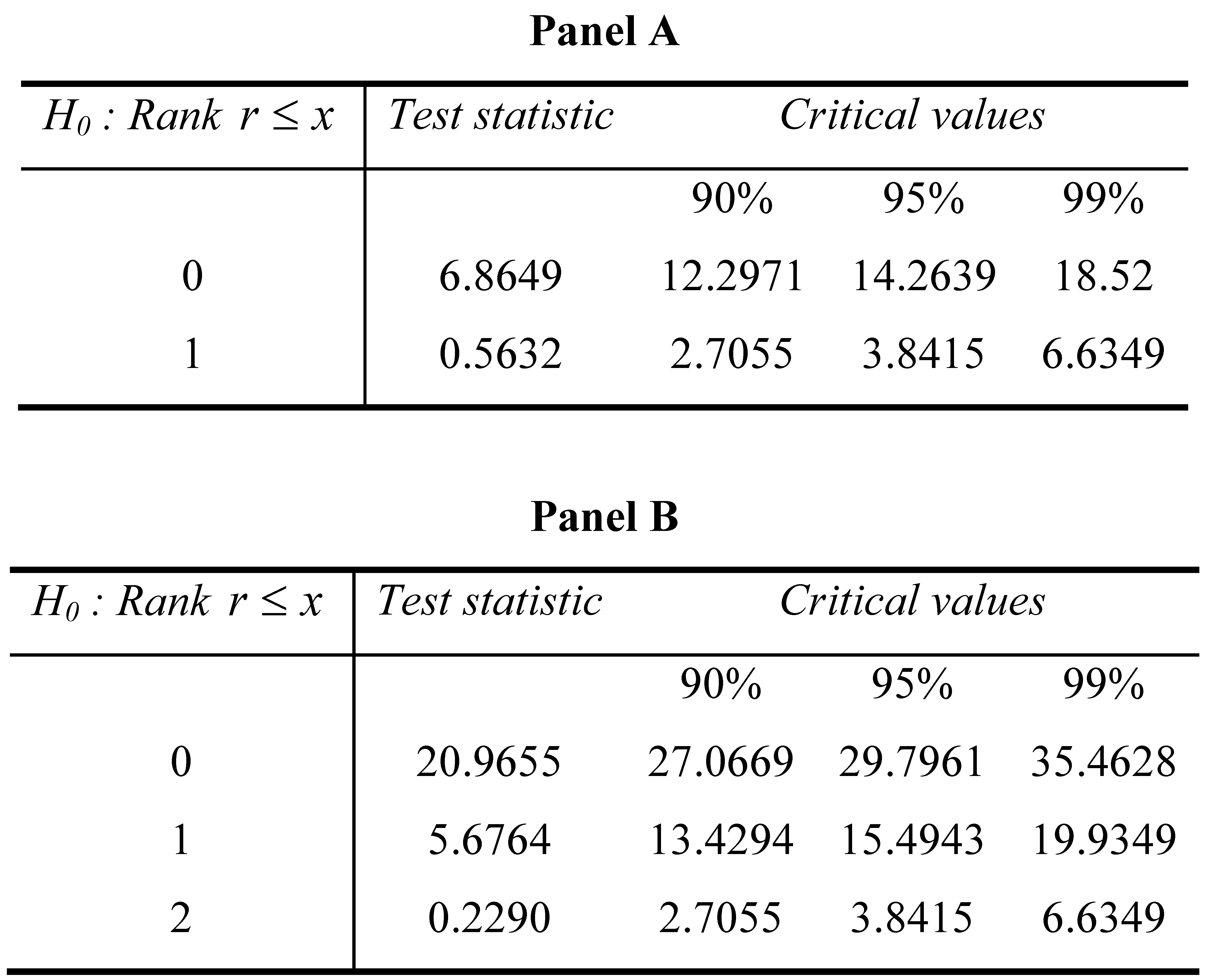
We discuss results from the tables below at the 0.05 significance level. For BVAR models we cannot reject the null hypothesis that there is no vector cointegrating stock prices and broad dividends (raw or deflated by marginal utility) for both the DJIA and S&P 500 data. Broad dividends alone do not sufficiently account for movements of stock prices, even in the long run. Hence, in what follows, we do not consider BVAR models any further.
We now compare results for raw stock prices and dividends with those deflated by marginal utility for the TVAR models only. We find that for models with raw data (Panel B in
Table 3 and
Table 4), we cannot reject the hypothesis that there is no vector cointegrating stock prices, broad dividends, and the output gap for either the DJIA or the S&P 500 data.
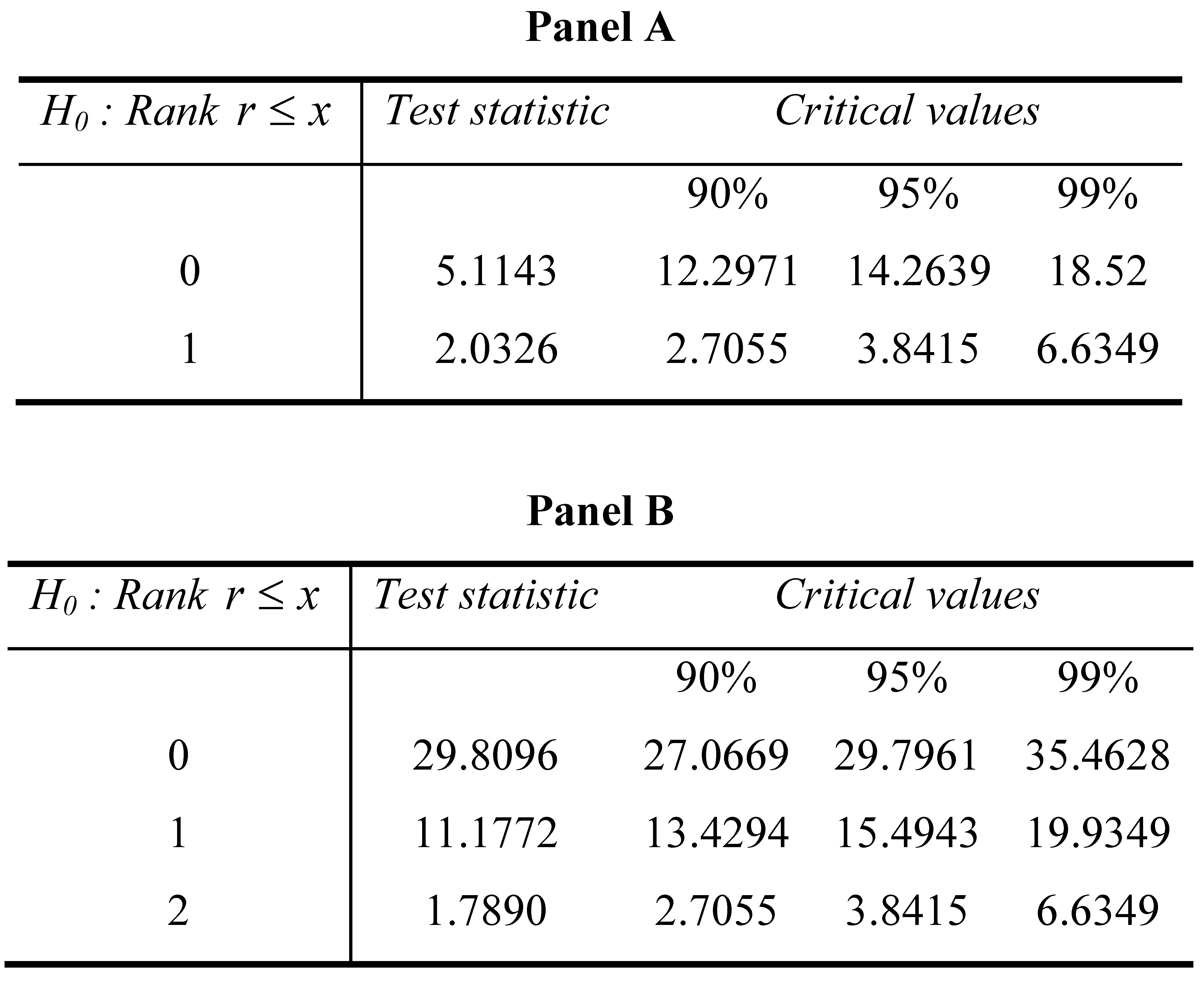
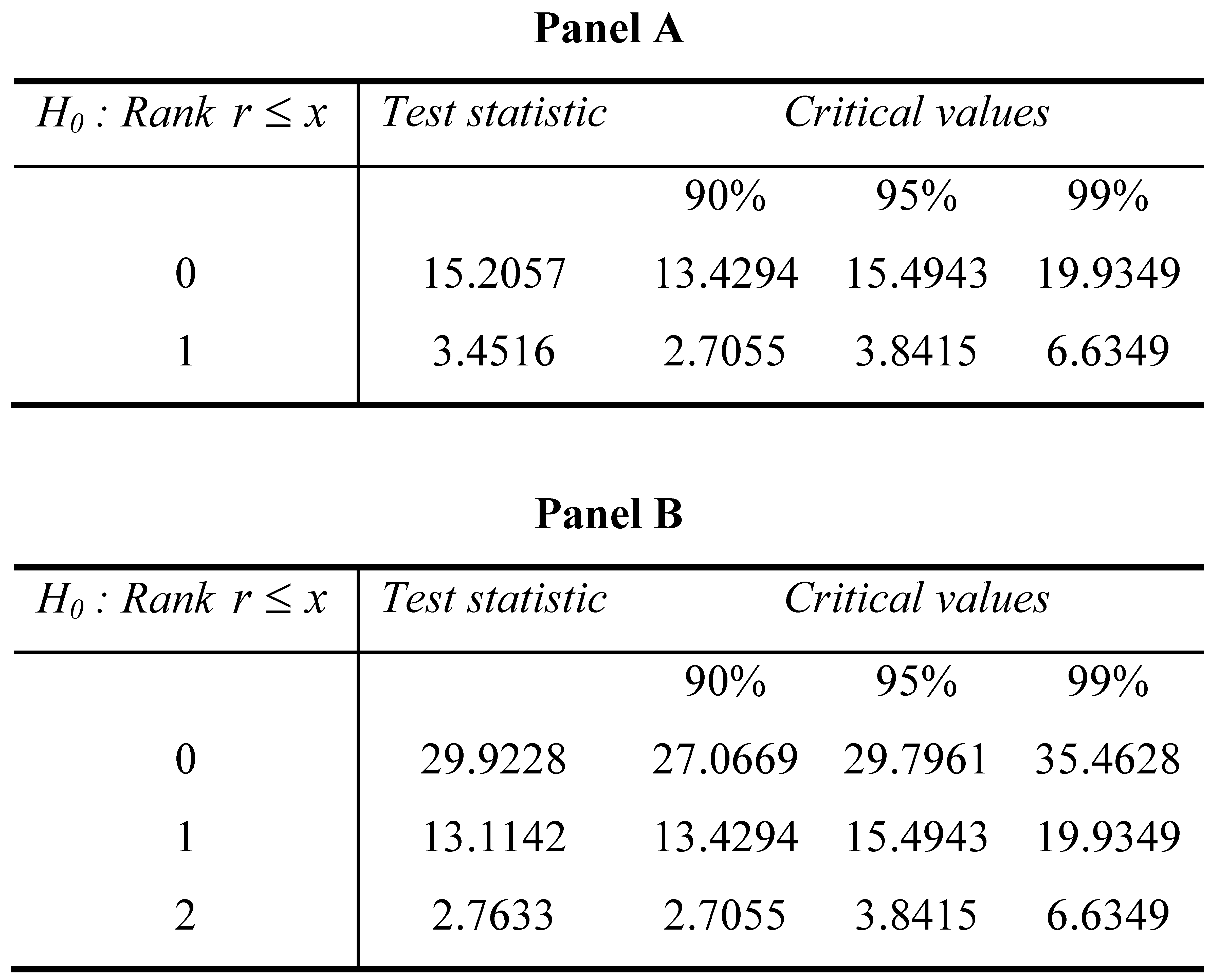
However, for models with deflated data (Panel B in
Table 5 and
Table 6), we reject that there is no cointegrating vector when stock prices and broad dividends are deflated by marginal utility. When we test for how many independent cointegrating vectors exist between these three variables, we cannot reject the hypothesis that there is zero or one cointegrating vector against the alternative that there are 2 vectors. We conclude that there is a single vector with which stock prices, broad dividends, and the output gap cointegrate.
When we make the third comparison of DJIA against S&P data, we do not find any qualitative difference in our statistical inferences whatsoever.
In summary, for both the DJIA and S&P data, deflated broad dividends along with the output gap can account for long run movements in deflated stock prices (cointegration between the three variables) within the TVAR framework. Broad dividends alone cannot rationalize long run movements in stock prices (no cointegration between the two). As discussed earlier in the previous section, output gap is largely orthogonal to broad dividends (whether deflated by marginal utility or not). Hence, it can account for the procyclical fluctuations in stock prices (whether deflated by marginal utility or not).
5.2.3. Tests for Periodically Collapsing Bubbles
As discussed in Phillips et al. (2007), evidence of cointegration does not preclude existence of periodically collapsing bubbles. In what follows, we test for such bubbles, but only with stock prices and broad dividends deflated by marginal utility since raw prices and dividends fail to exhibit cointegration in TVAR tests reported in the previous subsection.
Panel A of
Table 7 reports sup ADF
r statistics and ADF
1 statistics (equivalent to the single equation cointegration test statistic of Engle and Granger (1988)). Panel B provides critical values for both test statistics. The last column in Panel B reproduces critical values for the sup ADF
r test statistic obtained by Monte-Carlo simulations with 10,000 replications given in Phillips et al. (2007).
The ADF1 test statistics reported in the second row of Panel A are all less than the critical value at the 0.05 significance level. Thus, we cannot reject unit roots in the residuals of the single equation framework given in Equation (19). This means that we reject cointegration for both the DJIA and S&P series even when the output gap is included in the stock price equation. This is not totally consistent with the TVAR cointegration tests reported in the previous subsection where we did find cointegration between the three variables when prices and dividends are deflated by marginal utility.
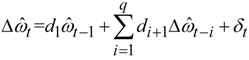
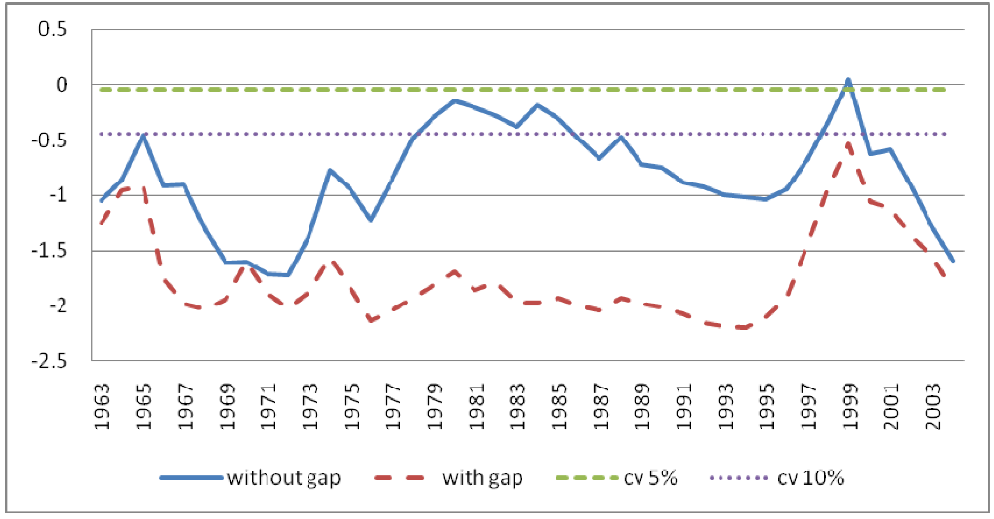
Although our dataset runs from 1949 to 2004, the ADFr test statistics are only computed from 1963 through 2004 by forward recursive regressions as in Phillips et al. (2007). Sup ADFr test statistics reported in the first row of Panel A show no explosive behavior in residuals from Equation (19) for the DJIA (with or without including the output gap). For the S&P series, however, both test statistics (for equations with and without the output gap) are larger than the 0.05 critical value. Thus, the null hypothesis of no explosive behavior in the residuals of Equation (19) is rejected. We therefore cannot rule out existence of periodically collapsing bubbles in S&P 500 data series. There is something in these stock prices that cannot be fully accounted for by both the fundamentals and macroeconomic factors considered here.
Next, we locate the timing of these periodically collapsing bubbles.
Figure 4 and
Figure 5 plot the ADF
r test statistics against time for the DJIA and S&P 500 series, respectively. The solid lines plot ADF
r test statistics for regression of stock prices on broad dividends only. The dashed lines plot these statistics for regression of stock prices on both broad dividends and the output gap. Critical values at the 0.05 and 0.10 significance levels are also shown.
As evident in the figures, compared with regressions of stock prices only on broad dividends, regressions on broad dividends and the output gap lower the ADFr test statistics. This is reasonable since, as reported in subsection 4.2.1, the output gap contains procyclical information on stock prices that is orthogonal to broad dividends.
From
Figure 4, with the output gap, there is no evidence of periodically collapsing bubbles in the DJIA data even at the 0.10 significance level. Without the output gap, however, at the 0.10 significance level, we find two periodically collapsing bubbles, one around 1980 and one in the late 1990s. From
Figure 5, we find periodically collapsing bubbles in S&P 500 data (with and without the output gap) in the late 1990s at the 0.05 significance level.
5.3. Discussion
Stock prices in the 1990s have been investigated extensively. There is debate over whether the run up in prices was due to irrational exuberance or due to reasonable expectations based on arrival of new technology, echoing a similar debate over the stock market run up in the 1920s (White 2006).
In the 1920s, a new industrial system emerged with continuous-process technology, large-scale new industry (automobiles), widespread use of internal combustion engines, and the spread of electricity. In New Levels in the Stock Market (1929), Charles Amos Dice (1929) argued that higher stock prices were the product of higher productivity. Dice identified increased expenditure on research and development and the application of modern management methods as prime factors behind the boom. Irving Fisher (1930) saw the stock market boom as justified by rising earnings, driven by systematic application of science and invention in industry, and the acceptance of new industrial management methods of Frederick Taylor (1911).
In the 1990s, rapid developments in computers, information technology, and biotechnology were heralded as placing the economy on a higher trajectory. This “new era” vision was supported by some economists. It potentially explains why we find periodically collapsing bubbles in S&P 500 data but not in DJIA, since there are more companies in S&P 500 than DJIA involved with those new technologies.
If one takes the view that the run up in stockprices is indeed caused by expectations of “new era”, then further research is needed to understand how investors build expectations for this kind of “new era”, and what kind of indicators we could use to model such expectations.
6. CONCLUSIONS
We investigate a model of stock prices, made up of fundamental and non-fundamental components. Fundamental component is formed as expected present value of all future broad dividends, discounted with a stochastic factor motivated by the consumption-based asset pricing model. Non-fundamental component is formed as a linear function of a macroeconomic factor, namely the output gap.
A trivariate VAR (TVAR) model for stock prices, broad dividends, and the output gap is used to test for cointegration between these three variables with Johansen (1988) and Stock and Watson (1988) procedures. A single equation model relating these three variables is used to test for periodically collapsing bubbles with the ADFr and Sup ADFr tests of Phillips et al. (2007).
We test the model with U.S. stock market data on annual DJIA and S&P 500 indices. We find that both stock price indices cointegrate with broad dividends and the output gap. At the same time, however, according to the sup ADFr test, we cannot rule out existence of periodically collapsing bubbles in S&P 500 data. The bubbles are in the 1990s booming period.


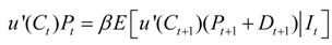

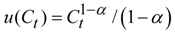 , where α is the coefficient of relative risk aversion. With this utility function, Equation (4) yields

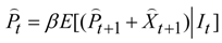
 . Given the discussion in Section 1.1, using Xt to denote broad dividends, this is re-expressed as

 , we can rewrite
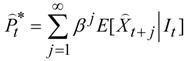
 to ensure finite prices.
 .
.

 .
.


