Modelling Insurance Claims During Financial Crises: A Systemic Approach

Abstract

In this paper, we introduce a generalised mutually exciting Hawkes process with random and independent jump intensities. This model provides a robust theoretical framework for modelling complex point processes and appropriately characterises the financial system, especially during periods of crisis. Based on this extended Hawkes process, we propose an insurance claim process and demonstrate that claim processes modelled as an aggregated process enable early detection of crises and inform optimal investment strategies in a financial system.

1. Introduction

The risk of contagion in economies and financial markets has become a significant source of concern among investors and businesses. The globalisation of economies means that businesses, now more than ever, are exposed to some common financial risks that threaten their profitability and existence. The global financial crisis of 2008 Sinha and Ahmad (2009) and the coronavirus pandemic Nicola et al. (2020) caused the collapse and near collapse of many companies that were hitherto classified as “too-big-to-fail” Strahan (2013).

There are many financial institutions whose purpose is to help economies and businesses manage their risks. The insurance industry is one such sector that plays the crucial role of insuring companies and institutions, and protecting them against unexpected losses that could be catastrophic to their survival. For effective risk management, businesses pay regular premiums to insurance companies that promise to pay their clients some compensation for unexpected losses. Insurance companies, then, invest the regular premiums received for higher returns to meet their financial obligations.

However, insurance companies operate within the same financial system as the businesses they insure and are, therefore, not immune to the happenings in the economy or in the system. Many insurance companies themselves have suffered greatly from the effects of global crises, be it economic, natural, or health crises Sinha and Ahmad (2009). Occasionally, these financial crises trigger a surge in simultaneous insurance claims from struggling businesses, a situation that places significant pressure on insurers and puts them in a very difficult and precarious financial position Schich (2009), necessitating robust risk management strategies and capital reserves to mitigate these systemic risks.

Generally, as a risk management strategy, insurance companies typically maintain a diverse client base spanning various industries and financial jurisdiction and therefore are subject to diverse risks. This diversification helps to mitigate the impact of risks that are unique to specific sectors or regions. However, in recent times, the nature of modern economies and economic systems is such that most businesses, regardless of their industries, are subjected to standard industry and systemic risks. This situation exposes all businesses to extreme operational risks which increases the likelihood of individuals, businesses, and institutions filing various insurance claims. The 2008 financial crisis and the coronavirus pandemic are classic examples of the potential impact that systemic crises can have on insurance claims. These crises led to an unprecedented spike in business interruption claims which were primarily driven by health-related business closures (i.e., lockdowns) and supply chain breakdowns, which severely interrupted a lot of businesses leading to a significant rise in claims Arnold (2021); Cummins and Weiss (2014).

The survival and profitability of insurance companies depend on their ability to accurately model claim occurrences in an increasingly complex global financial system and invest optimally to meet all their financial obligations. In insurance risk theory and the so called ruin theory, the classical Cramér-Lundberg model Lundberg (1903) and its numerous extensions Cheng and Seol (2020); Dassios and Zhao (2012); Stabile and Torrisi (2010); Swishchuk et al. (2021) have been used to model the arrival of insurance claims and, as a result, undertake the survival analysis of insurance companies. In the classical Cramér-Lundberg model, the claim process of an insurance company is given by:

$$C_t=\sum _{i=1}^{N_t}{X}_i,t\ge 0,$$

(1)

where $C_t$ is the total claims amount made to an insurance company up to time t, which are modelled as a compound Poisson process, and $X_{i}s$ are the individual claims amount made which are assumed to the independent and identically distributed (i.i.d.) random variables (r.v.) arriving according to a Poisson process $N(0,t]=N_t$ with constant intensity $\lambda$.

However, given the dynamics and complex nature of modern financial systems, many modifications of the Cramér-Lundberg claim process have been proposed and presented. In fact, Hawkes (2018); Stabile and Torrisi (2010); Swishchuk et al. (2021) argued that the memoryless property of the Poisson process makes it unsuitable for modelling claim arrivals since some claims may induce several other claims. They proposed, instead, to model the claims process using the Hawkes point process, which exhibits the self-exciting property that is more reflective of economic realities. The Hawkes process Hawkes (1971, 2018) has been widely applied in finance. To analyse the contagion effects of jumps on different asset prices, Aït-Sahalia et al. (2015) utilised the Hawkes processes in modelling financial contagion in asset prices. Similar applications of the Hawkes process in finance are highlighted in Bacry et al. (2015). In addition, Aït-Sahalia and Hurd (2015) used Hawkes processes to model contagion in investment analysis among many others. Also, Swishchuk (2017) used the Hawkes process to model insurance claims with similar variations to their models presented in Cheng and Seol (2020); Laub et al. (2015); Swishchuk et al. (2021). In Swishchuk et al. (2021), for example, Swishchuk developed a more general model of the insurance claims process using a compound Hawkes process, which they calibrated to empirical data for investment analysis.

In addition, a notable observation is that, often, claims processes of insurance institutions are modelled independently of each other, implying a lack of correlation and cross-excitation effects between insurance institutions Cheng and Seol (2020); Swishchuk et al. (2021). However, from empirical observations Sinha and Ahmad (2009); Şenol and Zeren (2020), insurance claims of different insurance institutions, especially during disasters or crises, tend to move in unison with extensive evidence of cross-excitation and correlation. In the next section, we present a few empirical observations of abrupt increases and similarities in claim processes between insurance institutions during crises.

2. Empirical Observations of Claims

Generally, obtaining insurance data is often challenging due to several factors. Insurance companies face stringent regulations, especially concerning data privacy and protection. Additionally, claims rate data are typically considered proprietary by insurers and regulatory authorities. Nevertheless, certain publicly accessible data sources can be utilised to support our empirical observations.

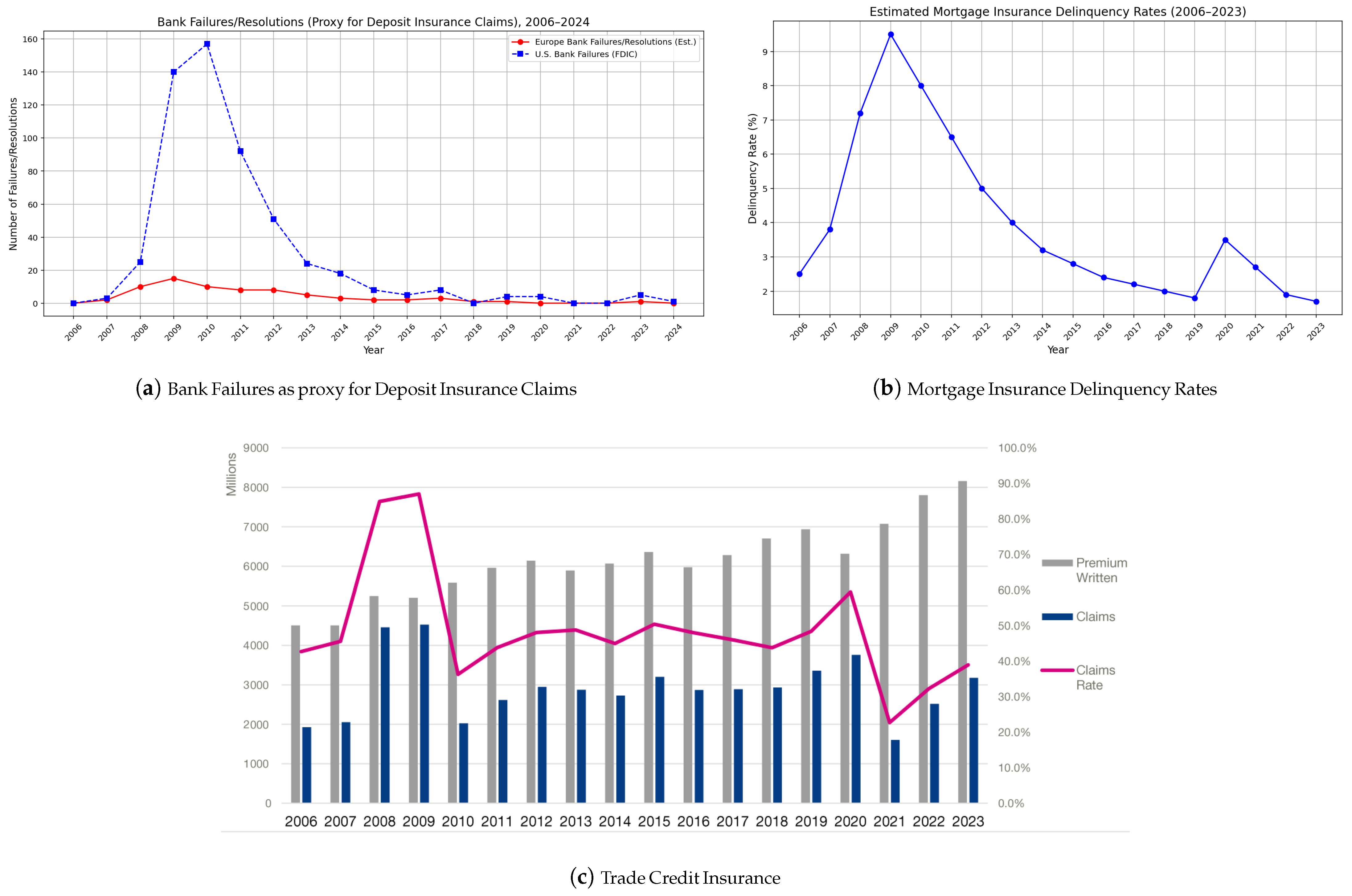
Figure 1 presents data and visualisations illustrating insurance claims or proxies of insurance claims across various insurance sectors and policies worldwide, covering the period from 2006 to 2024. Although not fully representative of the entire insurance industry, we observe from Figure 1 that insurance claims generally exhibit consistent global trends, albeit with varying magnitudes. During crises, a pronounced impact and clustering effect can be observed across multiple insurance institutions and sectors, accompanied by cross-excitation effects. These phenomena may stem from the shared financial environment in which these institutions operate or from similarities in their financing structures.

Overall, the figures consistently reveal a recognisable pattern across many insurance institutions. While specific segments of the industry may encounter distinct shocks or forms of crises, certain events are significant enough to reverberate throughout the broader financial system.

A notable insurance segment that is most affected during crises is the Business Interruption Insurance (BII). BII compensates businesses for income losses due to disruptions that affect businesses such as natural and human-made disasters, security crises and energy crises, equipment failures, pandemics, etc. Often times, businesses tend to suffer the most from systemic disasters, and therefore, the BII is one of the most impacted segments of the insurance industry during crises, as illustrated in Arnold (2021); Cummins and Weiss (2014).

Figure 1a, on the other hand, displays bank failures in the United States and Europe, sourced from Federal Deposit Insurance Corporation (FDIC) (2006–2024). These failures serve as a proxy for claims rates on insured deposits, as direct data on such claims are not publicly available. When a bank fails, the FDIC reimburses insured depositors, generating claims analogous to insurance payouts. The plot highlights periods of heightened bank failures, particularly during financial crises, underscoring the vulnerabilities in the insurance institutions within the banking sector.

Similarly, comprehensive data on mortgage insurance claims rates are not publicly accessible due to proprietary restrictions and regulatory constraints. However, Figure 1b leverages reports from Urban Institute (2006–2024), Mortgage Bankers Association (2006–2024), and other industry sources to use private mortgage insurance delinquency rates as a proxy for mortgage insurance claims in the United States. Mortgage insurance protects lenders against losses from borrower defaults, and delinquency rates provide a reasonable indicator of potential claims activity. Figure 1b reveals trends in the mortgage market, particularly during periods of economic downturn, offering insights into the housing sector’s impact on insurance claims.

Figure 1c depicts an aggregated claims rate of Trade Credit Insurance (TCI) from International Credit Insurance & Surety Association (ICISA) (2006–2023). Tread TCI is purchased by businesses to protect against losses from unpaid receivables when buyers fail to pay due to insolvency, bankruptcy, or other risks. During financial crises, liquidity challenges often lead to widespread buyer defaults, resulting in elevated TCI claims. This figure captures the trend of TCI claims, with significant increases during economic disruptions, reflecting the impact of crises in the financial system on Trade Insurance.

Broadly, the period before 2008 is often regarded as a time of relative financial stability, characterised by steady economic growth and minimal market shocks. As illustrated in Figure 1a–c, insurance claims rates across various sectors—BII, insured deposits, mortgage insurance, and TCI—remained low or moderate during this period. This stability is attributed to limited systemic disruptions and predictable risk exposures, reducing claims’ frequency and severity.

However, the global financial crisis, which began in late 2007 and intensified in 2008, profoundly impacted the financial and insurance industries. As evidenced in all panels of Figure 1, the crisis triggered a significant surge in claims across some insurance segments. For instance, BII claims rose due to business closures and supply chain disruptions caused by economic contraction. Insured deposit claims increased as bank failures peaked, with the FDIC reporting over 400 U.S. bank closures between 2008 and 2012. Mortgage insurance claims surged due to widespread homeowner defaults amid the subprime mortgage crisis. TCI claims spiked as corporate insolvencies soared, significantly increasing claims.

This synchronised rise in claims reflects significant cross-excitation effects, where shocks in one sector, such as the banking sector, amplified losses in others due to shared financial environments, interconnected supply chains, and systemic dependencies.

The years following the 2008 crisis were marked by recovery and reform. Tighter regulations were implemented to enhance financial stability and prevent similar crises. These measures, combined with monetary and fiscal interventions, fostered steady economic growth in the post-2008 period, as reflected in the stabilisation of insurance claims trends in Figure 1a–c. Claims rates generally returned to precrisis levels, with occasional fluctuations tied to localised events or crises (e.g., natural disasters or regional economic slowdowns).

The COVID-19 pandemic during 2020 disrupted this relative stability, causing a global economic and health crisis that led to another surge in insurance claims across multiple segments. As shown in most panels of Figure 1, the pandemic created pronounced peaks in claims, particularly claims from businesses, due to widespread business closures and lockdown measures. TCI also experienced a rise in claims as supply chain disruptions and economic uncertainty led to buyer insolvencies. The 2020 crisis further highlighted cross-excitation, as economic shutdowns in one region (e.g., Asia) affected global trade, amplifying TCI and BII claims worldwide.

These patterns provide compelling evidence of the insurance industry’s vulnerability to crises and the strong correlation of claims arrivals across different companies, sectors, and jurisdictions. Cross-excitation is particularly pronounced during systemic events, driven by shared exposures to shocks, interconnected financial systems, and globalised trade networks. The data in Figure 1a–c underscore the need for robust risk modelling and diversified portfolios to mitigate the impact of such correlated risks.

This paper presents a modified and more dynamic contagion insurance claim process based on the Hawkes process Bacry et al. (2015); Swishchuk et al. (2021) in an increasingly complex global financial system. We propose to model claims as an aggregated claim process based on the mutually exciting properties of the Hawkes process. We consider an aggregated d-dimensional claim process of all insurance institutions within a specified jurisdiction, whose ith entry is the claim process of insurance company i of interest with contagion effects on other dimensions of the process.

The model relaxes the assumption of independence of insurance claims processes of different institutions and extends the concept of contagion within the insurance industry and the economy, especially during periods of crisis. Consequently, during financial crises, we observe a general increase in the intensity of insurance claims, leading to higher-than-average claims throughout the financial system. Through multiple simulations, we show that the intensities of insurance claims experience random jumps, especially during global crises with cross-excitation effects on many insurance institutions.

3. Background

The Poisson process and its many extensions are among the most widely used point processes. The Hawkes process is an essential extension of the Poisson process that has seen many applications in insurance and finance risk theory. In this section, we introduce the Poisson and Hawkes point processes and illustrate some classical applications in insurance.

3.1. Poisson Process

An essential application of the Poisson process is in risk theory, which is used to count the occurrence of significant events such as insurance claims.

Definition 1

(Counting Process). Let $(\Omega ,\mathcal{F},{\left\{{\mathcal{F}}_t\right\}}_{t\ge 0},\mathbb{P})$ be a completely filtered probability space with $\omega \in \Omega$. Let ${\left\{T_n\right\}}_{n\in \mathbb{N}}=\{T_1\left(\omega \right),T_2\left(\omega \right),\dots \}$ be a sequence of increasing, independent and identically distributed (i.i.d.) random times. Then, we can define a process ${\left(N_t\right)}_{t\ge 0}$ that counts the number of random times ${\left\{T_n\right\}}_{n\ge 1}$ in an interval $[0,t]$ by:

$$N_t=\sum _{n\ge 1}{\mathbb{1}}_{\{T_n\left(\omega \right)\le t\}},t\ge 0,$$

(2)

where

$${\mathbb{1}}_{[T_n\left(\omega \right),\infty )}\left(t\right)=\left\{\begin{array}{cc}1\hfill & \mathit{if}{T}_n\ge t,\hfill \\ 0\hfill & \mathit{if}0\le t<T_n\hfill \end{array}\right..$$

For $n\ge 1$, and ${\left(T_n\right)}_{n\ge 1}$ is an increasing family of jump times of ${\left(N_t\right)}_{t\in {\mathbb{R}}_{+}}$ such that

$$\underset{k\to \infty }{lim}{T}_k=+\infty .$$

The process $N_t$ is called a counting process because it essentially counts the number of random times $T_n\left(\omega \right)$ occurring in the interval $[0,t]$. Therefore, $N_t$ has piecewise trajectories that increment by $+1$ at every count.

A defining property of a counting process is its intensity ${\lambda }_t$, which is the average number of counts in an interval $(0,t)$.

The parameter $\lambda >0$ of ${\left(N_t\right)}_{t\in {\mathbb{R}}_{+}}$ is given by:

$${\lambda }_t=\underset{h\to 0}{lim}{\displaystyle \frac{1}{h}}\mathbb{P}(N_t-N_{t+h}>0),$$

for some small time change increment h.

Definition 2

(Daley and Vere-Jones (2008)). Let ${\left(N_t\right)}_{t\in {\mathbb{R}}_{+}}$ be a point process and let ${\lambda }_t=\lambda >0$ be some constant. The counting process ${\left(N_t\right)}_{t\in {\mathbb{R}}_{+}}$ is called a Poisson process with intensity λ if all the following conditions hold:

• $N_0=0$;
• $N_t$ has independent and stationary increments;
• The number of arrivals or increments in any interval of length $\tau >0$ follows a Poisson distribution with parameter $\lambda \tau$.

Therefore, the short-time asymptotic of the Poisson process is given by:

$$\mathbb{P}[N_h=n]=\left\{\begin{array}{cc}{e}^{-\lambda t}\simeq 1-\lambda h+o\left(h\right),h\to 0\hfill & \mathrm{if}n=0,\hfill \\ \lambda h{e}^{-\lambda h}\simeq \lambda h,h\to 0\hfill & \mathrm{if}n=1\hfill \end{array}\right..$$

(3)

However, in many extensions of the Poisson process, the intensity can be made time-dependent, in which case we have:

$$\mathbb{P}(N_t-N_s=n)=e^{-{\int }_s^t\lambda \left(u\right)du}{\displaystyle \frac{{\left({\int }_s^t\lambda \left(u\right)du\right)}^n}{n!}},n=0,1,2,\dots$$

So that, assuming that $\lambda \left(t\right)$ is a continuous function of time t, we have in particular, as h tends to zero,

$$\mathbb{P}[N_{t+h}-N_t=n]=\left\{\begin{array}{cc}exp\left(-{\int }_t^{t+h}\lambda \left(u\right)du\right)\simeq 1-\lambda \left(t\right)h+o\left(h\right),\hfill & \mathrm{if}n=0\hfill \\ exp\left(-{\int }_t^{t+h}\lambda \left(u\right)du\right)\left({\int }_t^{t+h}\lambda \left(u\right)du\right)\simeq \lambda \left(t\right)h+o\left(h\right),\hfill & \mathrm{if}n=1\hfill \\ o\left(h\right),\hfill & \mathrm{if}n>1\hfill \end{array}\right.,$$

(4)

3.2. Hawkes Process

We have seen how the intensity of the Poisson process can be extended to a time-dependent intensity parameter. The Hawkes process is a path-dependent extension of the Poisson process with cross-excitation properties, where each count increases the likelihood of future counts. Using the Hawkes process Laub et al. (2015), an event’s occurrence, known as the parent event, may trigger the occurrence of other events. Therefore, the most essential property of the Hawkes process is the path-dependent intensity process ${\lambda }_t$.

Definition 3

(Laub et al. (2015)). Let $(\Omega ,\mathcal{F},{\left\{{\mathcal{F}}_t\right\}}_{t\ge 0},\mathbb{P})$ be a completely filtered probability space and let $N={\left\{N_t^i\right\}}_{t\ge 0}^{i=1,\dots ,d}$ be a $d$-dimensional point process. Suppose that, for each i, $N={\left\{N_t^i\right\}}_{t\ge 0}^{i=1,\dots ,d}$ satisfies the following:

$$\mathbb{P}[N_{t+h}^i-N_t^i=n|{\mathcal{F}}_t]=\left\{\begin{array}{cc}1-{\lambda }_t^{i}h+o\left(h\right),\hfill & \mathit{if}n=0\hfill \\ {\lambda }_t^{i}h+o\left(h\right),\hfill & \mathit{if}n=1\hfill \\ o\left(h\right),\hfill & \mathit{if}n>1\hfill \end{array}\right.,$$

(5)

where ${\lambda }_t^i$ is the ${\mathcal{F}}_t$-conditional intensity process of $N^i$ for each i. Then, the point process N is called a Hawkes process if its intensity process ${\lambda }_t$ is given by:

$$\begin{array}{ccc}\hfill \mathbb{E}\left[{\mathcal{N}}_i(\omega ,A)\right]& ={\lambda }_t^i={\lambda }_0^i+\sum _{j=1}^d{\int }_0^t{\varphi }^{i,j}(t-s){\mathcal{N}}_j\left(ds\right),\hfill & \hfill \mathit{for}i,j=1,\dots ,d\end{array}$$

(6)

where ${\lambda }_0^i\ge 0$ are the background intensities or the average Poisson intensity for the immigrants of $N_{i,t}$. ${\varphi }^u(t-s)\ge 0$ for all $u\ge 0$ is the mutually exciting or cross-excitation kernel function that describes the impact of a parent event of type $j=1,\dots ,d$ on events of type $i=1,\dots ,d$, and where $T_{j,r}$ is the time the rth event of type j occurred. The kernel function is appropriately chosen to reflect our intended model.

4. The Model

Let $(\Omega ,\mathcal{F},{\left\{{\mathcal{F}}_t\right\}}_{t\ge 0},\mathbb{P})$ be a completely filtered probability space with $\omega \in \Omega$. Let ${\left\{T_n^{h_i}\right\}}_{n\in \mathbb{N}}=\{T_1^{h_i}\left(\omega \right),T_2^{h_i}\left(\omega \right),\dots \}$ and ${\left\{T_n^{p_i}\right\}}_{n\in \mathbb{N}}=\{T_1^{p_i}\left(\omega \right),T_2^{p_i}\left(\omega \right),\dots \}$ and be sequences of increasing i.i.d. random times and let ${\left\{X_n^{h_i}\right\}}_{n\in \mathbb{N}}=\{X_1^{h_i}\left(\omega \right),X_2^{h_i}\left(\omega \right),\dots \}$ and ${\left\{X_n^{p_i}\right\}}_{n\in \mathbb{N}}=\{X_1^{p_i}\left(\omega \right),X_2^{p_i}\left(\omega \right),\dots \}$ a sequence of random variables such that $X_k^{h_i}\left(\omega \right)$ is revealed at $T_k^{h_i}\left(\omega \right)$ and $X_k^{p_i}\left(\omega \right)$ is revealed at $T_k^{p_i}\left(\omega \right)$ for all $i\in \mathbb{N}$ (i.e., $X_k^{h_i}$ is ${\mathcal{F}}_{T_k^{h_i}}$-measurable and $X_k^{p_i}$ is ${\mathcal{F}}_{T_k^{p_i}}$-measurable). Note that the superscript $p_i$ in the variables $T^{p_i}$ and $X^{p_i}$ is an abbreviation for jump in the i-th element.

Suppose further that ${\left\{T_n^{h_i}\right\}}_{n\in \mathbb{N}}$ represents event times that arrive according to a Hawkes process $N^{h_i}$ with intensity process ${\lambda }_t^{h_i}$ so that $T_n^{h_i}$ is the n-th event time of the process. We also suppose that ${\left\{T_n^{p_i}\right\}}_{n\in \mathbb{N}}$ represent some other event times that arrive according to a Poisson process $N^{p_i}$ with the constant rate ${\lambda }^p$ with $N^{p_i}$ being independent of $N^{h_i}$. It is important to note that by our definitions above, there are i.i.d. random variables $X^{h_i}$ and $X^{p_i}$ that are, respectively, associated with each of the random times $T^i$ and $T^{p_i}$.

From the definitions above, ${(T_n^{h_i},X_n^{h_i})}_{n\ge 0}^{i=1,\dots ,d}$ together with ${(T_n^{p_i},X_n^{p_i})}_{n\ge 0}^{i=1,\dots ,d}$ form a random configuration of points that can be used to define a marked point process $N={\left\{N_n^i\right\}}_{n\ge 0}^{i=1,\dots ,d}$ whose intensity process is given by:

$${\lambda }^i(t,x|{\mathcal{F}}_t)={\lambda }_t^{h_i}(t,x|{\mathcal{F}}_t)+{\lambda }^{p_i}(t,x|{\mathcal{F}}_t).$$

(7)

Let $(0,t]\times \mathcal{E}$ be a product space where $\mathcal{E}$ is the mark space. For each $i=1,\dots ,d$, the random events ${(T_n^{h_i}\left(\omega \right),X_n^{h_i}\left(\omega \right))}_{n\ge 0}\subset (0,t]\times {\mathcal{E}}^{h_i}$ is such that $T^{h_i}$ represents the arrival time of insurance claims and $X^{h_i}$ represents the mark of the insurance claim made to insurance company i in the group of d different insurers. Similarly, ${(T_n^{p_i}\left(\omega \right),X_n^{p_i}\left(\omega \right))}_{n\ge 0}\subset (0,t]\times {\mathcal{E}}^{p_i}$ is such that $T^{p_i}$ represents jump times in the intensity process ${\lambda }^i$ of the marked Point Process $N^i$ with $X^{p_i}$ representing the jump sizes of the in intensity process ${\lambda }^i$ of $N^i$.

Conceptually, the d-dimensional generalised Hawkes Process, N with aggregated intensity $\Lambda$ presented in this work, is an aggregated claim process of a group of insurers in an economy or in a well-defined financial system where each dimension represents the claim process of a constituent member of the group.

The intensity of the claim $\lambda (t,x)$ is important in modelling insurance claims. Suppose without loss of generality that the intensity in Equation (7) can be rewritten as:

$$\begin{array}{cc}\hfill {\lambda }^i(t,x|{\mathcal{F}}_t)& ={\lambda }_t^{h_i}(t,x|{\mathcal{F}}_t)+{\lambda }^{p_i}(t,x|{\mathcal{F}}_t),\hfill \end{array}$$

(8)

$$\begin{array}{cc}\hfill & \hspace{1em}\hspace{1em}\hspace{1em}\hspace{1em}\hspace{1em}\hspace{1em}={\lambda }^{g{h}_i}\left(t\right|{\mathcal{F}}_t)f^{g{h}_i}\left(x\right|{\mathcal{F}}_t)+{\lambda }^{p_i}{f}^{g{p}_i}\left(x\right|{\mathcal{F}}_t),\hfill \end{array}$$

(9)

where ${\lambda }^{g{h}_i}$ is the “non-crises” ground intensity process of insurance claims, $f^{g{h}_i}$ is the density of the non-crises marks of insurance claims, ${\lambda }^{p_i}$ is the Poisson constant intensity of the jumps observed during periods of crises, and $f^{g{p}_i}$ is the density intensity of the jumps.

As rightly observed in Swishchuk et al. (2021), some economic or non-economic events may be significant enough to engender multiple insurance claims, causing a ripple effect on the insurer and in the financial system; hence, the adoption of the Hawkes ground intensity process in our model of insurance claims arrival during “non-crises” periods.

However, during financial crises, we often observe a significant and abrupt increase in the intensity of insurance claims, which sometimes leads to above-average claims. The surge in aggregated claims rate during crisis periods, as observed in Figure 1, is a reflection of the financial environment in which the insurance companies operate and a strong indication, yet, of a possible correlation between internal and external insurance claims. These increments in the number of claims are often unexpected and not necessarily attributable to previous claims, as assumed in Swishchuk et al. (2021) and other Hawkes-inspired models Hawkes (2018); Laub et al. (2015).

Financial crises and uncertainties often lead to panic and reactionary decisions from financial institutions and investors. This panic and reactionary decisions by investors are major contributors to jumps and clustering effects observed in prices, which further exacerbate an already dire situation for many businesses. During these periods, insurers tend to err on the side of caution and, as a risk management strategy, prepare for the possibility of numerous claims while still expecting a fall in their expected returns. Hence, Equation (8) accounts for the significant and unexpected increase in the intensities of claims during crisis periods.

Suppose that the intensity process in Equation (8) can be represented in the following form:

$$\begin{array}{cc}\hfill {\lambda }^i(t,x|{\mathcal{F}}_t)& ={\lambda }^{g{h}_i}\left(t\right|{\mathcal{F}}_t)f^{g{h}_i}\left(x\right|{\mathcal{F}}_t)+{\lambda }^{p_i}{f}^{g{p}_i}\left(x\right|{\mathcal{F}}_t),\hfill \\ \hfill {\lambda }^i(t,x|{\mathcal{F}}_t)& =\left({\lambda }_0^i+\sum _{j=1}^d{\eta }_{i,j}{\int }_{(0,t]\times \mathcal{X}}{\rho }_{i,j}\left(x\right){\kappa }_{i,j}^h(t-s){\mathcal{N}}_j(ds,dx)\right)f^{g{h}_i}\left(x\right|{\mathcal{F}}_t)+\sum _{i:T^{p_i}\le t}(\Delta {\lambda }^i){\kappa }^{p_i},\hfill \\ \hfill {\lambda }^i(t,x|{\mathcal{F}}_t)& =\left({\lambda }_0^i+\sum _{j=1}^d{\eta }_{i,j}{\int }_{(0,t]\times \mathcal{X}}{\rho }_{i,j}\left(x\right){\kappa }_{i,j}^h(t-s){\mathcal{N}}_j(ds,dx)\right)f^{g{h}_i}\left(x\right|{\mathcal{F}}_t)+\sum _{i:T^{p_i}\le t}{X}^{p_i}{\kappa }^{p_i},\hfill \end{array}$$

Hence:

$$\begin{array}{c}\hfill {\lambda }^i(t,x|{\mathcal{F}}_t)=\left({\lambda }_0^i+\sum _{j=1}^d{\eta }_{i,j}{\int }_{(0,t]\times \mathcal{X}}{\rho }_{i,j}\left(x\right){\kappa }_{i,j}^h(t-s){\mathcal{N}}_j(ds,dx)\right)f^{g{h}_i}\left(x\right|{\mathcal{F}}_t)\\ \hfill +{\int }_{(0,t]\times \mathcal{X}}b\left(x^{p_i}\right){\kappa }^{p_i}{J}_{{\Lambda }^i}^i(ds\times dx),\end{array}$$

(10)

where

$$\Delta {\lambda }^i=\lambda \left(T_n^{p_i}\right)-\lambda \left(T_n^{p_i-}\right)=X^{p_i},\mathrm{where}\lambda \left(T_n^{p_i-}\right)=\underset{s\to T_n^{p_i-}}{lim}\lambda \left(s\right)$$

for each $i=1,\dots ,d$, where ${\lambda }_0^i$ is the background or baseline intensity, ${\eta }_{i,j}\ge 0$ are the branching coefficients, ${\rho }_{i,j}:{\mathbb{R}}_{+}\mapsto {\mathbb{R}}_{+}$ are the impact functions or the strength of the cross-excitation, and ${\kappa }_{i,j}^h:\mathbb{R}\mapsto {\mathbb{R}}_{+}$ and ${\kappa }^{p_i}:\mathbb{R}\mapsto {\mathbb{R}}_{+}$ are the decays of the kernel and the decay of jumps. $J_{\Lambda }$ is the Poisson random measure on $[0,t]\times {\mathbb{R}}^d$ with intensity ${\nu }_{{\Lambda }^i}^i={\nu }^i\left(dx\right)dt={\upsilon }^i{f}^{g{p}_i}\left(dx\right)dt$, where ${\upsilon }^i$ in the intensity of the Poisson process $M^i$.

To ensure existence and uniqueness, the following normalising conditions must hold as verified in Liniger (2009):

$${\int }_0^{\infty }\kappa \left(\tau \right)d\tau =1,{\int }_0^{\infty }\tau \kappa \left(\tau \right)d\tau <\infty ,{\int }_0^{\infty }{\rho }_{i,j}{f}_{g_h}^i\left(x\right|{\mathcal{F}}_t)dx=1,$$

(11)

and

$${\int }_{|x^i|\le 1}{\left|x^i\right|}^2{\nu }^i\left(dx\right)<\infty ,{\int }_{|x^i|\ge 1}{\nu }^i\left(dx\right)<\infty ,$$

(12)

for all $i,j=1,\dots ,d$.

4.1. The Impact Function and Jump Size Distribution

Different events impact subsequent events depending on their nature, size, and time of occurrence. Therefore, the excitation function ${\rho }_{i,j}$ of an event of type i may differ significantly or marginally from that of another event.

To prevent negative impact and huge jumps that may disrupt our model and also to ensure that it satisfies the conditions of existence in Equation (11), we adopt a linear and normalised impact function of ${\rho }_{i,j}$ so that $\mathbb{E}\left[{\rho }_{i,j}\left(x\right)\right]=1$. We consider a normalised polynomial impact function given by:

$${\rho }_{i,j}\left(x\right|{\mathcal{F}}_t)={\displaystyle \frac{1+b_{i,j}x}{1+b_{i,j}\mathbb{E}\left[x\right|{\mathcal{F}}_t]}}.$$

To completely specify the moments, the distribution of the mark of the events must be specified. Generally, claim events with significant cross-excitation effects are rare but extreme events. Similarly, financial crises, by their nature, are also rare, but they come with a significant impact. Therefore, a natural candidate for the distribution of the marks or jump sizes distribution in our intensity process is the generalised Pareto distribution (GPD):

$$F\left(x\right|{\mathcal{F}}_t)=\left\{\begin{array}{c}1-{\left(1+\xi {\displaystyle \frac{x-\mu }{\sigma }}\right)}^{-{\displaystyle \frac{1}{\xi }}},\xi \ne 0,\hfill \\ 1-exp\left(-\xi {\displaystyle \frac{x-\mu }{\sigma }}\right),\xi =0,\hfill \end{array}\right.\Rightarrow f\left(x\right|{\mathcal{F}}_t)=\left\{\begin{array}{c}{\displaystyle \frac{1}{\sigma }}{\left(1+\xi {\displaystyle \frac{x-\mu }{\sigma }}\right)}^{-{\displaystyle \frac{1}{\xi }}-1},\xi \ne 0,\hfill \\ {\displaystyle \frac{1}{\sigma }}exp\left(-{\displaystyle \frac{x-\mu }{\sigma }}\right),\xi =0\hfill \end{array}\right.$$

(13)

where f is the density function, $\xi \ge \mu$ is the shape parameter, $\sigma \ge 0$ is the scale parameter, and $\mu$ is the location parameter. It is important to note that the parameters will be chosen to ensure positive values. Also note that when $\xi =0$, the GDP reduces to the exponential distribution. When $\xi <1$, the mean of the GPD exists and is given by:

$$\mathbb{E}\left[x\right]=\mu +{\displaystyle \frac{\sigma }{1-\xi }}.$$

Therefore, the impact function to be computed is given by:

$${\rho }_{i,j}\left(x\right|{\mathcal{F}}_t)={\displaystyle \frac{(1+b_{i,j}x)(1-\xi )}{1-\xi +b_{i,j}\mu (1-\xi )+b_{i,j}\sigma }}.$$

(14)

The shape and scale parameters are estimated as constant parameters to simplify the model.

4.2. Decay Kernel

The notable differences in the extensions of the Hawkes process are in the choice of the ground intensity process ${\lambda }_g$ and the kernel function. As observed in (Bacry et al., 2015; Laub et al., 2015), a common choice of a kernel function ${\varphi }^{i,j}$ is the exponential decaying kernel function such that ${\varphi }^{i,j}(t-s)={\beta }_{i,j}{e}^{-{\alpha }_i(t-s)},s<t$ for $i,j=1,\dots ,d$, which properly reflects the self-exciting and mutually exciting properties of the Hawkes process. With this choice of kernel function, a jump in the point process increases its intensity by $\beta$, an impact which, subsequently, decays at a rate of $\alpha$.

In a well-regulated and efficient market, it is expected that market prices and levels will adjust quickly to the arrival of new information, differing only by the intensity of the impact function or the size of the events. Hence, we adopt the usual exponential specification of the decay function that ensures that the first assumption of Equation (11) above is verified:

$${\kappa }_{i,j}^h\left(\tau \right)={\delta }_{i,j}{e}^{-{\delta }_{i,j}(\tau -s)},\mathrm{and},{\kappa }^{p_i}\left(\tau \right)=e^{-{\gamma }_i(\tau -s)},$$

(15)

where ${\delta }_i$ is the parameter controlling the intensity of the decay of the impact of previous events.

This parametrisation also appropriately reflects the process’s self and mutual excitation properties, its clustering properties, and the jumps observed during periods of extreme economic distress. An event of type i arrives at an average rate of ${\lambda }_0^i$ and generates descendant events at rate $\eta$, which becomes an ancestor event to generate other immigrant events as it decays out.

Proposition 1.

Let N be a Hawkes process defined in Equation (10) and let Equation (11) hold. Then, the ${\mathcal{F}}_t$-compensator of our generalised Hawkes process N is given by:

$$\begin{array}{c}\hfill {\lambda }^i=\left({\lambda }_0^i+\sum _{j=1}^d{\int }_{(0,t]\times \mathcal{X}}{\displaystyle \frac{{\alpha }_{i,j}}{{\beta }_{i,j}}}(1+b_{i,j}x){\delta }_{i,j}{e}^{-{\delta }_{i,j}(t-s)}{\mathcal{N}}_j(ds,dx)\right)f^{g{h}_i}\left(x\right|{\mathcal{F}}_t)\\ \hfill {\int }_{(0,t]\times \mathcal{X}}\left({\displaystyle \frac{(1+b_{i,j}^{p_i}x)(1-\xi )}{1-\xi +b_{i,j}^{p_i}\mu (1-\xi )+b_{i,j}^{p_i}\sigma }}\right)e^{-{\gamma }_i(\tau -s)}{J}_{{\Lambda }^i}(ds\times dx),\end{array}$$

(16)

and if $\mu =0$

$$\begin{array}{c}\hfill {\lambda }^i=\left({\lambda }_0^i+\sum _{j=1}^d{\int }_{(0,t]\times \mathcal{X}}{\displaystyle \frac{{\alpha }_{i,j}}{{\beta }_{i,j}}}(1+b_{i,j}x){\delta }_{i,j}{e}^{-{\delta }_{i,j}(t-s)}{\mathcal{N}}_j(ds,dx)\right)f^{g{h}_i}\left(x\right|{\mathcal{F}}_t)+\\ \hfill {\int }_{(0,t]\times \mathcal{X}}\left({\displaystyle \frac{(1+b^{p_i}x)(1-\xi )}{1-\xi +b^{p_i}\sigma }}\right)e^{-{\gamma }_i(\tau -s)}{J}_{{\Lambda }^i}(ds\times dx),\end{array}$$

(17)

for each $i,j=1,\dots ,d$.

Proof. 

Consider N, the d-dimensional generalised Hawkes process defined in Equation (10) with the corresponding intensity ${\lambda }_t$ given by:

$$\begin{array}{c}\hfill {\lambda }^i(t,x|{\mathcal{F}}_t)=\left({\lambda }_0^i+\sum _{j=1}^d{\eta }_{i,j}{\int }_{(0,t]\times \mathcal{X}}{\rho }_{i,j}\left(x\right){\kappa }_{i,j}^h(t-s){\mathcal{N}}_j(ds,dx)\right)f^{g{h}_i}\left(x\right|{\mathcal{F}}_t)\\ \hfill +{\int }_{(0,t]\times \mathcal{X}}b\left(x^{p_i}\right){\kappa }^{p_i}{J}_{{\Lambda }^i}^i(ds\times dx),\end{array}$$

If we let

$${\eta }_{i,j}={\displaystyle \frac{{\alpha }_{i,j}}{{\beta }_{i,j}}}\left({\displaystyle \frac{1-\xi +b_{i,j}\mu (1-\xi )+b\sigma }{1-\xi }}\right),{\rho }_{i,j}={\displaystyle \frac{(1+b_{i,j}x)(1-\xi )}{1-\xi +b_{i,j}\mu (1-\xi )+b_{i,j}\sigma }}.$$

$$b\left(x^{p_i}\right)={\displaystyle \frac{(1+b^{p_i}x)(1-\xi )}{1-\xi +b_{i,j}\mu (1-\xi )+b_{i,j}\sigma }},{\kappa }_{i,j}^h\left(\tau \right)={\delta }_{i,j}{e}^{-{\delta }_{i,j}(\tau -s)},\mathrm{and},{\kappa }^{p_i}\left(\tau \right)=e^{-{\gamma }_i(\tau -s)}$$

$$\begin{array}{c}{\lambda }^i=\left({\lambda }_0^i+\sum _{j=1}^d{\int }_{(0,t]\times \mathcal{X}}{\displaystyle \frac{{\alpha }_{i,j}}{{\beta }_{i,j}}}(1+b_{i,j}x){\delta }_{i,j}{e}^{-{\delta }_{i,j}(t-s)}{\mathcal{N}}_j(ds,dx)\right)f^{g{h}_i}\left(x\right|{\mathcal{F}}_t)+\hfill \\ \hfill {\int }_{(0,t]\times \mathcal{X}}\left({\displaystyle \frac{(1+b^{p_i}x)(1-\xi )}{1-\xi +b^{p_i}\mu (1-\xi )+b^{p_i}\sigma }}\right)e^{-{\gamma }_i(\tau -s)}{J}_{{\Lambda }^i}(ds\times dx),\end{array}$$

and if $\mu =0$ it follows that:

$$\begin{array}{c}{\lambda }^i=\left({\lambda }_0^i+\sum _{j=1}^d{\int }_{(0,t]\times \mathcal{X}}{\displaystyle \frac{{\alpha }_{i,j}}{{\beta }_{i,j}}}(1+b_{i,j}x){\delta }_{i,j}{e}^{-{\delta }_{i,j}(t-s)}{\mathcal{N}}_j(ds,dx)\right)f^{g{h}_i}\left(x\right|{\mathcal{F}}_t)+\hfill \\ \hfill {\int }_{(0,t]\times \mathcal{X}}\left({\displaystyle \frac{(1+b^{p_i}x)(1-\xi )}{1-\xi +b^{p_i}\sigma }}\right)e^{-{\gamma }_i(\tau -s)}{J}_{{\Lambda }^i}(ds\times dx),\end{array}$$

Furthermore, this equation is well defined if ${\displaystyle \frac{\xi -1}{\sigma }}<b^{p_i}$ and ${\eta }_{i,j}$ so that $\mathbb{E}\left[{\lambda }^i\right]<\infty$. □

5. Parameter Estimation and Goodness-of-Fit Tests

The maximum likelihood estimation technique is used to estimate the parameters of the intensity process ${\lambda }^i(t,x|{\mathcal{F}}_t)$ in Equation (8). Therefore, to compute the likelihood function, mainly the log-likelihood function associated with the intensity process, we denote by $\theta$ the vector of the parameters to be estimated, and we let $(t_1,x_1),\dots ,(t_{N_g\left(T\right)},x_{N_g\left(T\right)})$ be realisations of the d-dimensional process N and its corresponding d-dimensional intensity process $\Lambda$.

Using the definitions of the intensity process $\Lambda$, the ground intensity process ${\Lambda }_g$ and the density function f of the claim events and the distribution of the jumps in the intensity process, then from Proposition (7.3.III) in Daley et al. (2003), the appropriate parameter $\theta$ is chosen to maximise the intensity function as follows.

Proposition 2

(Contagion Hawkes Likelihood function). Let N be a d-dimensional Hawkes process a d-dimensional intensity process defined in Equation (8), then the log-likelihood function is given by:

$$\begin{array}{c}\hfill log\left(L\right)=\sum _{i=1}^d\sum _{j=1}^{N_g^{h_i}\left(T\right)}log\left\{{\lambda }^{h_i}\left(t_j\right|{\mathcal{F}}_t)\right\}+\sum _{i=1}^d\sum _{j=1}^{N_g^{h_i}\left(T\right)}log\left\{f^{g{p}_i}\left(x_j\right|{\mathcal{F}}_t)\right\}-\sum _{i=1}^d{\int }_0^T{\lambda }^{h_i}\left(s\right|{\mathcal{F}}_s)ds\\ \hfill +\sum _{i=1}^d\sum _{j=1}^{M^{p_i}\left(T\right)}log\left\{{\lambda }^{p_i}\right\}-\sum _{i=1}^d{\lambda }^{p_i}T+\sum _{i=1}^d\sum _{j=1}^{M^{p_i}}log\left\{f^{g{p}_i}\left(x_j\right|{\mathcal{F}}_t)\right\}.\end{array}$$

(18)

Proof. 

From Equation (8), we have that:

$$\begin{array}{cc}\hfill {\lambda }^i(t,x|{\mathcal{F}}_t)& ={\lambda }_t^{h_i}(t,x|{\mathcal{F}}_t)+{\lambda }^{p_i}(t,x|{\mathcal{F}}_t),\hfill \\ \hfill & ={\lambda }^{g{h}_i}\left(t\right|{\mathcal{F}}_t)f^{g{h}_i}\left(x\right|{\mathcal{F}}_t)+{\lambda }^{p_i}{f}^{g{p}_i}\left(x\right|{\mathcal{F}}_t).\hfill \end{array}$$

Therefore, the log-likelihood function of the intensity can be computed as the sum of the log-likelihoods of the two parts. From Proposition (7.3.III) in Daley et al. (2003), the Hawkes part is given by:

$$\begin{array}{cc}\hfill L& =\prod _{i=1}^d\left[\left(\prod _{j=1}^{N_g^{h_i}\left(T\right)}{\lambda }^{h_i}(t_j,x_j|{\mathcal{F}}_{t_j})\right)exp\left\{-{\int }_0^T{\int }_{\mathcal{X}}{\lambda }^{h_i}(s,x|{\mathcal{F}}_s)ds{\mu }_x\left(dx\right)\right\}\right],\hfill \\ \hfill & =\prod _{i=1}^d\left[\left(\prod _{j=1}^{N_g^{h_i}\left(T\right)}{\lambda }^{h_i}(t_j,x_j|{\mathcal{F}}_{t_j})\right)exp\left\{-{\int }_0^T{\lambda }^{g{h}_i}\left(s\right|{\mathcal{F}}_s)ds\right\}\right],\hfill \\ \hfill log\left(L\right)& =log\left\{\prod _{i=1}^d\left(\prod _{j=1}^{N_g^{hi}\left(T\right)}{\lambda }^{hi}(t_j,x_j|{\mathcal{F}}_{t_j})\right)\right\}+log\left\{\prod _{i=1}^{d}exp\left\{-{\int }_0^T{\lambda }^{hi}\left(s\right|{\mathcal{F}}_s)ds\right\}\right\},\hfill \\ \hfill log\left(L\right)& =\sum _{i=1}^d\sum _{j=1}^{N_g^{hi}\left(T\right)}log\left\{{\lambda }^{g{h}_i}\left(t\right|{\mathcal{F}}_t)\right\}+\sum _{i=1}^d\sum _{j=1}^{N_g^{h_i}\left(T\right)}log\left\{f^{g{h}_i}\left(x\right|{\mathcal{F}}_t)\right\}-\sum _{i=1}^d{\int }_0^T{\lambda }^{h_i}\left(s\right|{\mathcal{F}}_s)ds,\hfill \end{array}$$

and the Poisson-jump part of the process is given by:

$$\begin{array}{cc}\hfill L& =\prod _{i=1}^d\left[\left(\prod _{j=1}^{M^{p_i}\left(T\right)}{\lambda }^{p_i}(t_j,x_j|{\mathcal{F}}_{t_j})\right)exp\left\{-{\int }_0^T{\int }_{\mathcal{X}}{\lambda }^{p_i}(s,x|{\mathcal{F}}_s)ds{\nu }_x\left(dx\right)\right\}\right],\hfill \\ \hfill & =\prod _{i=1}^d\left[\left(\prod _{j=1}^{M^{p_i}\left(T\right)}{\lambda }^{p_i}(t_j,x_j|{\mathcal{F}}_{t_j})\right)exp\left\{-{\int }_0^T{\lambda }^{p_i}\left(s\right|{\mathcal{F}}_s)ds\right\}\right],\hfill \\ \hfill log\left(L\right)& =log\left\{\prod _{i=1}^d\left(\prod _{j=1}^{M_g^{p_i}\left(T\right)}{\lambda }^{p_i}(t_j,x_j|{\mathcal{F}}_{t_j})\right)\right\}+log\left\{\prod _{i=1}^{d}exp\left\{-{\int }_0^T{\lambda }^i\left(s\right|{\mathcal{F}}_s)ds\right\}\right\},\hfill \\ \hfill log\left(L\right)& =\sum _{i=1}^d\sum _{j=1}^{M_g^i\left(T\right)}log\left\{{\lambda }^{p_i}\right\}+\sum _{i=1}^d\sum _{j=1}^{M_g^{p_i}\left(T\right)}log\left\{f^{g{p}_i}\left(x_j\right|{\mathcal{F}}_t)\right\}-\sum _{i=1}^d{\int }_0^T{\lambda }^{p_i}ds,\hfill \\ \hfill log\left(L\right)& =\sum _{i=1}^d\sum _{j=1}^{M_g^i\left(T\right)}log\left\{{\lambda }^{p_i}\right\}+\sum _{i=1}^d\sum _{j=1}^{M_g^{p_i}\left(T\right)}log\left\{f^{g{p}_i}\left(x_j\right|{\mathcal{F}}_t)\right\}-\sum _{i=1}^d{\lambda }^{p_i}T.\hfill \end{array}$$

Hence:

$$\begin{array}{c}\hfill log\left(L\right)=\sum _{i=1}^d\sum _{j=1}^{N_g^{h_i}\left(T\right)}log\left\{{\lambda }^{h_i}\left(t_j\right|{\mathcal{F}}_t)\right\}+\sum _{i=1}^d\sum _{j=1}^{N_g^{h_i}\left(T\right)}log\left\{f^{g{p}_i}\left(x_j\right|{\mathcal{F}}_t)\right\}-\sum _{i=1}^d{\int }_0^T{\lambda }^{h_i}\left(s\right|{\mathcal{F}}_s)ds\\ \hfill +\sum _{i=1}^d\sum _{j=1}^{M^{p_i}\left(T\right)}log\left\{{\lambda }^{p_i}\right\}-\sum _{i=1}^d{\lambda }^{p_i}T+\sum _{i=1}^d\sum _{j=1}^{M^{p_i}}log\left\{f^{g{p}_i}\left(x_j\right|{\mathcal{F}}_t)\right\}\end{array}$$

which is well defined considering our assumptions in Equation (11). □

6. Contagion Claim Process

The GHP enables us to develop a claim process for an insurance company in the face of systemic risk, especially during financial crises.

Suppose that insurance claims $X_i$s arrive at an insurance company i following the ith entry of a d-dimensional GHP defined in Equation (10), then the claim process for company i is given by:

$$C_t^i=\sum _{n=1}^{N_t^i}{X}_n^i,\mathrm{for}i=1,\dots ,d$$

(19)

As a result, by an abuse of notation, the aggregated claim process is given by:

$$C_t=\left[\begin{array}{c}\sum _{n=1}^{N_t^1}{X}_n^1\\ \sum _{n=1}^{N^2}{X}_n^2\\ ⋮\\ \sum _{n=1}^{N^d}{X}_n^d\end{array}\right]=\sum _{n=1}^N{X}_n,$$

(20)

where $N:={\left\{N_n^i\right\}}_{n\ge 0}^{i=1,\dots ,d}$ is a d-dimensional GHP that counts the number of random times in $[0,T]$ an event of type $\mathcal{X}$ happens. The intensity of the process N is given by:

$$\begin{array}{c}{\lambda }^i=\left({\lambda }_0^i+\sum _{j=1}^d{\int }_{(0,t]\times \mathcal{X}}{\displaystyle \frac{{\alpha }_{i,j}}{{\beta }_{i,j}}}(1+b_{i,j}x){\delta }_{i,j}{e}^{-{\delta }_{i,j}(t-s)}{\mathcal{N}}_j(ds,dx)\right)f^{g{h}_i}\left(x\right|{\mathcal{F}}_t)+\hfill \\ \hfill {\int }_{(0,t]\times \mathcal{X}}\left({\displaystyle \frac{(1+b^{p_i}x)(1-\xi )}{1-\xi +b^{p_i}\sigma }}\right)e^{-{\gamma }_i(\tau -s)}{J}_{{\Lambda }^i}(ds\times dx),\end{array}$$

Our aggregated claim model can be fitted to insurance claims data for appropriate goodness of fit tests and forecasting. Many estimation techniques have been proposed for Hawkes models, including Bacry et al. (2016); Kirchner (2017); Lee and Seo (2017).

Each dimension represents the claim process of an insurance company i whose claims have cross-excitation effects on other process dimensions. Modelling insurance claims as an aggregated process presents many advantages. In this way, insurers can take worthy notes of the happenings of competing insurers and take preventive measures to avoid them. It also facilitates the early detection and prevention of crises and enables insurers to take strict measures to minimise the cross-excitation parameters for effective risk management.

7. Simulation of Jump Intensity GHP Model

Based on Ogata’s modified thinning algorithm Ogata (1998); Swishchuk (2021), we generate point processes whose intensity is given by Equation (10). This algorithm is inspired by Algorithm 7.5.IV of Daley et al. (2003) with some modifications to account for the Poisson jumps in the intensities. We, therefore, introduce two simulation algorithms; for the first, we introduce a simulation algorithm of a univariate GHP $N_t$ whose intensity process ${\lambda }_t$ is given by Equation (10), and the second simulation algorithm consists of a two-dimensional or multivariate process, whose intensity process $\lambda$ is given by Equation (10) with $d=2$.

7.1. Simulation of a 1D GHP

Consider a one-dimensional claim process as in Equation (19), where $N^i$ is a generalised Hawkes process with its intensity given by Equation (10). The algorithm below is employed to simulate the GHP:

• Set the initial conditions by defining the parameters:
  • $T_0=0$, start time of all the processes;
  • ${\lambda }_{T_0^i}={\lambda }_0^i=0.9$, the initial and baseline intensity of the process;
  • Choose the excitation parameters, say $\eta \rho =0.5$, and the excitation decay, say $\delta =1.0$, to determine how much and how quickly past events influence future ones;
  • Specify the time interval, say 100 s;
  • Optionally, set a maximum intensity ${\lambda }_{\max }$ for computational efficiency in the thinning algorithm;
  • Create an empty list of event times and set $t=T_0=0$.
• Generate Event Times:
  • Compute the current conditional intensity ${\lambda }_t$, which includes the baseline ${\lambda }_0$ plus contributions from all past events using the triggering function;
  • Propose a potential next event time t by drawing from an exponential distribution with rate $\lambda$ and upper bound ${\lambda }_t$;
  • Evaluate ${\lambda }_t$ at the proposed time;
  • Generate a uniform random number $U\sim$uniform(0,1) and accept the event at t if $U\le \lambda \left(t\right)/{\lambda }_{\max }$, and otherwise, reject it and try again;
  • If accepted, add t to the list of event times and update the intensity function—if rejected, propose another t;
  • Repeat until the desired end time (e.g., 100 s) is reached.
• Generate Jump Times and Magnitudes:
  • Use a Poisson process to generate jump times over the interval $[0,T]$;
  • For each jump time, draw a random magnitude from the chosen distribution;
  • The jumps decay exponentially at a rate $\gamma$.
• Update the Intensity Function by adding the jump and its decay contribution to ${\lambda }_t$:

  $${\lambda }_{T_{k+1}^i}^i=({\lambda }_{T_k^i}^i-a)e^{-\delta (T_{k+1}^i-T_k^i)}+Y_{k+1}^i+1_{U_i<t}{J}_{T_{k+1}^{p_i}}^i{e}^{-\gamma (t-T_{k+1}^{p_i})},$$

  where $Y_{k+1}^i\sim$ is the generalised Pareto distribution, where $\xi =0$ and $\mu =0$ (i.e., the exponential distribution) represent the impact of previous realisations of the point process and $J_{T_{k+1}^{p_i}}=\Delta {\lambda }^i=\lambda \left(T_{k+1}^{p_i}\right)-\lambda \left(T_{k+1}^{p_i-}\right)\sim$. The generalised Pareto distribution represents the jump sizes in the intensity whose arrival times follow a Poisson process with intensity ${\nu }^{p_i}$.
• Update the count in the Hawkes process N at the new arrival time by:

  $$N_{T_{k+1}^i}^i=N_{T_k^i}^i+1.$$

7.2. Simulation of a 2D GHP

Similarly, we consider a two-dimensional claim process as in Equation (19) where $N^i$ is a generalised Hawkes process with its intensity given by Equation (10) for $d=2$. The algorithm below is used to simulate the GHP.

• Set the initial conditions by defining the parameters:
  • $T_0=0$, start time of the process;
  • Initiate the processes by specifying the baseline intensity of all the dimensions of the process, say ${\lambda }_{T_0^1}={\lambda }_0^1=0.9$ and ${\lambda }_{T_0^2}={\lambda }_0^2=2.2$;
  • Choose the excitation parameters say ${\rho }_{1,1},{\rho }_{1,2},{\rho }_{2,1},{\rho }_{2,2}$ and the decay of the excitation say ${\delta }_{1,1},{\delta }_{1,2},{\delta }_{2,1},{\delta }_{2,2}$ to determine how much and how quickly past events influence future ones;
  • Specify the time interval, say 100 s;
  • Optionally, set a maximum intensity ${\lambda }_{\max }^1$ for each i for computational efficiency in the thinning algorithm;
  • Create an empty list of event times and set $t^u=T_0^i=0$ for each i.
• Generate Event Times Using Ogata’s Thinning Algorithm (this algorithm simulates events by comparing a time-varying intensity to a uniform random process):
  • Compute the current conditional intensity ${\lambda }_t^i$, which includes the baseline ${\lambda }_0^i$ plus contributions from all past events using the triggering function;
  • Propose a potential next event time $t^i$ by drawing from an exponential distribution with rate ${\lambda }^i$ an upper bound on ${\lambda }_t^i$;
  • Evaluate ${\lambda }_t^i$ at the proposed time;
  • Generate a uniform random number $U^i\sim$uniform(0,1) and accept the event at t if $U^i<{\lambda }^i\left(t\right)/{\lambda }_{\max }^i$, and otherwise, reject it and try again for all $i\in 1,\dots ,d$;
  • If accepted, add t to the list of event times and update the intensity function—if rejected, propose another t;
  • Repeat until the desired end time (e.g., 100 s) is reached.
• Generate Jump Times and Magnitudes for each i;
  • Use a Poisson process to generate jump times over the interval $[0,T]$;
  • For each jump time, draw a random magnitude from the chosen distribution;
  • The jumps decay exponentially at a rate ${\gamma }^i$.
• Update the Intensity Function by adding the jump and its decay contribution to ${\lambda }_t^i$;

  $${\lambda }_{T_{k+1}^i}^i=({\lambda }_{T_k^i}^i-a)e^{-\delta (T_{k+1}^i-T_k^i)}+Y_{k+1}^i+1_{U_i<t}{J}_{T_{k+1}^{p_i}}^i{e}^{-\gamma (t-T_{k+1}^{p_i})},$$

  where $Y_{k+1}^i\sim$ is the generalised Pareto distribution where $\xi =0$ and $\mu =0$ (i.e., the exponential distribution) represent the impact of previous realisations of the point process and $J_{T_{k+1}^{p_i}}=\Delta {\lambda }^i=\lambda \left(T_{k+1}^{p_i}\right)-\lambda \left(T_{k+1}^{p_i-}\right)\sim$ is the generalised Pareto distribution, which represents the jump sizes in the intensity whose arrival times follow a Poisson process with intensity ${\nu }^{p_i}$.
• Update the count in the Hawkes process N at the new arrival time by:

  $$N_{T_{k+1}^i}^i=N_{T_k^i}^i+1.$$

7.3. Simulation Analysis

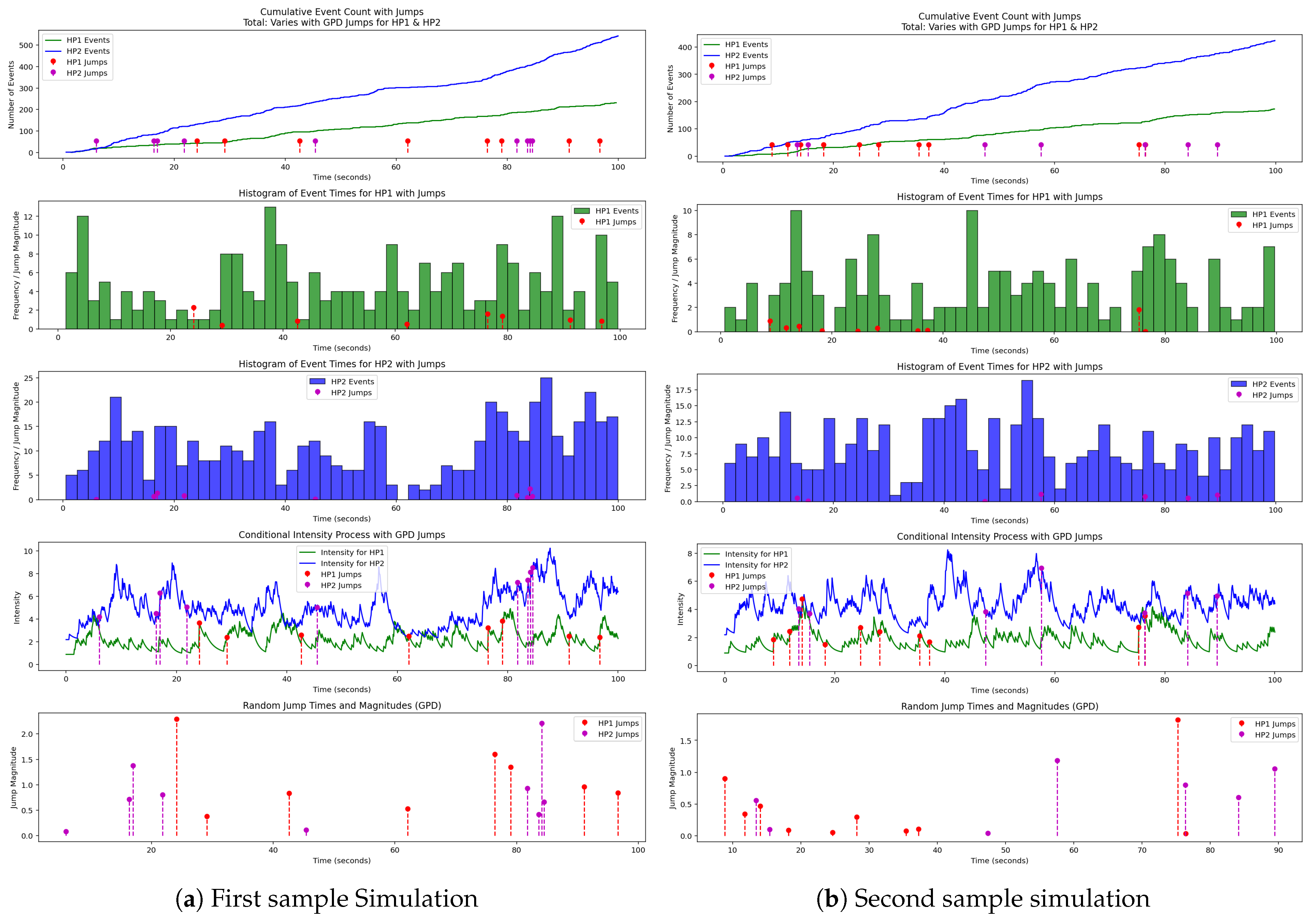
The univariate and multivariate simulations present many interesting observations. From the simulated graphs, we observe the clustering effects of the Hawkes part of the process and the significant but rare effects of the random GPD jumps observed in the process.

It is worth reiterating that in the classical Hawkes Process and its extensions, the intensities are path-dependent, and they increase significantly or marginally in response to jumps in the original process N. However, in great economic recessions and financial crises, numerous insurance claims are made almost simultaneously, abruptly increasing the intensity of insurance claims.

We note that the increments in the intensities are not only attributable to previous jumps as assumed in the original Hawkes Process $N_t$ but also attributable to some random jumps due to a compound Poisson process J. This is reminiscent of what is observed during financial crises. These random jumps significantly increase the intensities of our model, leading to an increase in the number of insurance claims with some cross-excitation effects. This is characteristic of the financial system during global or localised financial crises, where we observed a significant jump in the intensities of insurance claims and an above-average increment of monetary claims.

Generally, claims can be classified as minor or significant, with varying effects on subsequent claims and the insurance company. In addition, depending on the prevailing economic conditions in the global or local financial system, intensities of insurance claims experience significant jumps due to the volatility of the prevailing economic conditions. For example, in Figure 2b at times 40 and 80 and in Figure 3b at times 25 and 85, the univariate and multivariate processes experienced random jumps with significant jump magnitudes on the intensities of the Point processes. These jumps in the intensities are characteristic of the effects of more essential claims, possibly due to significant events such as natural disasters or major financial crises. We observe some significant cross-excitation effects on the intensities and some increments in the respective Point processes due to these jumps in the intensities.

Also, in Figure 2a,b and Figure 3a,b, we observe a similar random jump in the intensity of insurance company 1, which, although it affects the company’s claims, does not significantly affect insurance company 2. This could be because insurance institutions may have different areas of specialisation, which may affect the institutions differently. It could also be due to some insurance institutions operating in a system more resistant to external shocks than others, or companies adequately diversifying their risks or clientele.

In our model and simulations, we assumed that the marks in the intensities follow a generalised Pareto distribution because of the cascading effects of the events. Similarly, in the simulation, we assumed that the jump sizes in the intensities of the process also follow the generalised Pareto distribution because events that lead to jumps in the intensity process are extreme. However, in practice, this model can be adapted to many situations, and a goodness-of-fit test can be undertaken together with some simulations. The adaptations mean that the distributions can be varied to accommodate different realities and conditions, and some variables can be redefined.

8. Risk Model Based on GHP and Ruin Probability

Based on our generalised Hawkes process, we can derive an aggregated risk model in a financial system. Let $N={\left(N_t^i\right)}_{t\ge 0}^{i=1,\dots ,d}$ be a Hawkes process of d dimensions with a d dimension intensity ${\left({\lambda }_t^i\right)}_t^{i=1,\dots ,d}$ described by Equation (16). Suppose also that ${\left(X_k^i\right)}_{k\ge 0}$ are non-negative i.i.d. random variables that represent the claim amount for each i.

Let $N_t$ be the number of claims made up to time $t\ge 0$, which we model as the GHP in Equation (8) with its associated intensity process ${\lambda }_t$ in Equation (10). Let us also consider a sequence ${\left(X_n\right)}_{n\ge 1}$ of non-negative independent, identically distributed random variables represent insurance claim amounts up to time $t\ge 0$, which arrive according to the GHP $N_t$. Then, the aggregated claim process is given by:

$$C_t^i=\sum _{k=1}^{N_t^i}{X}_k^i,\mathrm{for}i=1,\dots ,d$$

(21)

The claim process can also be rewritten as:

$$C_t^i=Y_{N_t^i}^i,t\in {\mathbb{R}}_{+}$$

(22)

where ${\left(Y_k^i\right)}_{k\ge 1}$ is the sequence of random variables independent of ${\left(N_t\right)}_{t\in {\mathbb{R}}_{+}}$ given by:

$$Y_k^j=\sum _{i=1}^k{Z}_i^j$$

with $Y_0=0$.

Definition 4.

Consider the GHP $N_t$ with its associated intensity process ${\lambda }_t$ and the claim process C(t) defined above. Then, the surplus process ${\left(S_t\right)}_{t\ge 0}$ is given by:

$$S\left(t\right)=x+f\left(x\right)-C\left(t\right)$$

(23)

where $x\ge 0$ is the amount of the initial reserves or capital and $f:\mathbb{R}\mapsto \mathbb{R}$ is an increasing function that represents the premium income received between time 0 and time $t>0$, and C is the claim process.

An integral part of the claims process is the study of our model’s survival or ruin probability. Therefore, we are interested in the probability that the surplus process $S\left(t\right)$ falls below zero at some point t in the future. Therefore, we wish to find the ruin time t given by:

$$\tau =inf\{t>0:R(t)<0|R\left(0\right)=x\}.$$

(24)

Also, the ruin probability is given by:

$$\Phi \left(t\right)=\mathbb{P}(\tau \le t|R\left(0\right)=x),$$

(25)

where $\tau$ is the ruin time, so that the infinite ruin probability is given by:

$$\Phi (\infty )=\underset{t\to \infty }{lim}\Phi \left(t\right)=\underset{t\to \infty }{lim}\mathbb{P}(\tau \le t|R\left(0\right)=x).$$

(26)

9. Conclusions

This paper introduced a generalised, mutually exciting Hawkes process whose intensities exhibit random Poisson jumps. This model extends the traditional Hawkes process used in finance by capturing the heightened uncertainty during global financial disruptions, where sharp and unexpected increases in intensities lead to a surge in claims, characteristic of the modern and interconnected global financial system.

The model provides a theoretical framework for modelling insurance claims and is designed to mirror the complex dynamics of crises within the financial system. The proposed d-dimensional claim process offers a powerful tool for insurance companies and serves as an early warning system to navigate the intricacies of modern, interdependent financial networks. Our results highlight the model’s potential to strengthen risk assessment and management, particularly in turbulent market conditions.

We plan to refine the model for future work by incorporating time-varying covariates to account for correlations and other market-specific factors that may influence claim intensities. Additionally, we aim to explore the integration of machine learning techniques to improve the predictive accuracy of the early detection system, particularly for identifying the onset of crises. Furthermore, empirical validation using real-world insurance claim datasets from diverse financial markets will further test the model’s suitability and robustness.