Ensemble Multi-Expert Forecasting: Robust Decision-Making in Chaotic Financial Markets

Abstract

Financial time series in volatile markets often exhibit non-stationary behavior and signatures of stochastic chaos, challenging traditional forecasting methods based on stationarity assumptions. In this paper, we introduce a novel multi-expert forecasting system (MES) that leverages ensemble machine learning techniques—including bagging, boosting, and stacking—to enhance prediction accuracy and support robust risk management decisions. The proposed framework integrates diverse “weak learner” models, ranging from linear extrapolation and multidimensional regression to sentiment-based text analytics, into a unified decision-making architecture. Each expert is designed to capture distinct aspects of the underlying market dynamics, while the supervisory module aggregates their outputs using adaptive weighting schemes that account for evolving error characteristics. Empirical evaluations using high-frequency currency data, notably for the EUR/USD pair, demonstrate that the ensemble approach significantly improves forecast reliability, as evidenced by higher winning probabilities and better net trading results compared to individual forecasting models. These findings contribute both to the theoretical understanding of ensemble forecasting under chaotic market conditions and to its practical application in financial risk management, offering a reproducible methodology for managing uncertainty in highly dynamic environments.

1. Introduction

Financial time series are characterized by high volatility, non-stationarity, structural breaks and abrupt regime shifts. Foundational work on ARCH models has demonstrated the importance of capturing time-varying volatility (Chou & Kroner, 1992), while regime-switching frameworks allow one to model sudden market transitions (Hamilton, 2010). Classical forecasting techniques—ARMA, ARIMA and GARCH—remain cornerstones of empirical econometrics: ARMA presumes covariance stationarity following mean adjustment; ARIMA absorbs low-frequency trends via differencing; and GARCH models the conditional second moments under a (weakly) stationary conditional mean (Box & Jenkins, 1970; Engle, 1982; Chou & Kroner, 1992).

In financial decision science it is crucial to distinguish risk and uncertainty. Risk refers to situations where outcome probabilities are known (allowing quantification), whereas uncertainty—in the Knightian sense—implies that both outcomes and their distributions are unknown (Knight, 1921). Traditional VaR-style metrics address only risk; residual uncertainty must be mitigated through structural model diversity. Accordingly, our MES delivers probabilistic outputs that quantify risk, while the heterogeneity of its experts hedges against model uncertainty that cannot be captured by any single specification.

A further complication is the weak-form Efficient-Markets Hypothesis (EMH) for liquid currency pairs: one-minute EUR/USD returns approximate a martingale with near-zero linear predictability (Fama, 1970). Purely linear models frequently fail to capture the rich nonlinear and chaotic dynamics observed in financial markets. Granger (2008) highlights the limitations of traditional single-model approaches and advocates the use of ensemble methods to improve forecast accuracy in economics. Zhou’s comprehensive treatment of ensemble learning algorithms (Zhou, 2025) underpins many of the strategies we employ in our multi-expert system (MES). Moreover, Avramov and Chordia (2006) show that adaptive and ensemble techniques can compensate for model misspecification and significantly enhance predictive power under conditions of structural instability.

Finally, high-frequency data (HFD) exacerbate microstructure noise and quote-bounce effects that spoil the i.i.d. error assumptions of low-frequency econometrics (Zhang et al., 2005). Our empirical design therefore aggregates 1 min ticks into minute-bars, applies variance-stabilizing transformations, and uses heteroscedastic robust error estimates throughout (see Section 2.2). These precautions, combined with the ensemble architecture, allow us to confront the dual challenge of risk and residual uncertainty in a market that is close to weak-form efficient yet demonstrably chaotic.

In this context, recent advances in deep learning–augmented ensembles have shown potential. Han et al. (2024) propose a hybrid framework that integrates GARCH-type models with LSTM architectures to model volatility clusters and temporal dependencies in non-stationary series. Similarly, Li et al. (2022) apply ensemble deep learning for metro passenger flows, yet their methodology is equally relevant for high-frequency financial data, where concept drift and seasonality pose significant barriers to generalization.

Other works (A. A. Musaev et al., 2021; A. Musaev & Grigoriev, 2022) emphasize the importance of accounting for structural breaks and abrupt changes through model adaptation and segmentation. This is aligned with the findings of (Cretarola et al., 2020), who incorporate attention-based mechanisms to track shifting patterns in Bitcoin prices, demonstrating that ignoring non-stationarity significantly deteriorates forecast quality.

Moreover, Nguyen and Thu (Nguyen & Thu, 2018) explore support vector machines (SVMs) for forex prediction and highlight the algorithm’s ability to capture nonlinearities. However, they also acknowledge limitations in adapting to fast-changing dynamics, thus making a case for multi-model aggregation rather than relying on a single ML architecture.

Contemporary reviews and meta-analyses (Ayitey et al., 2023) further reveal a shift toward multi-expert and hybrid modeling approaches, especially in volatile markets where traditional methods frequently fail. These reviews advocate for combining statistical foundations with ML-based learning and soft computing techniques (e.g., fuzzy logic, evolutionary learning), especially when operating in highly noisy and chaotic financial environments.

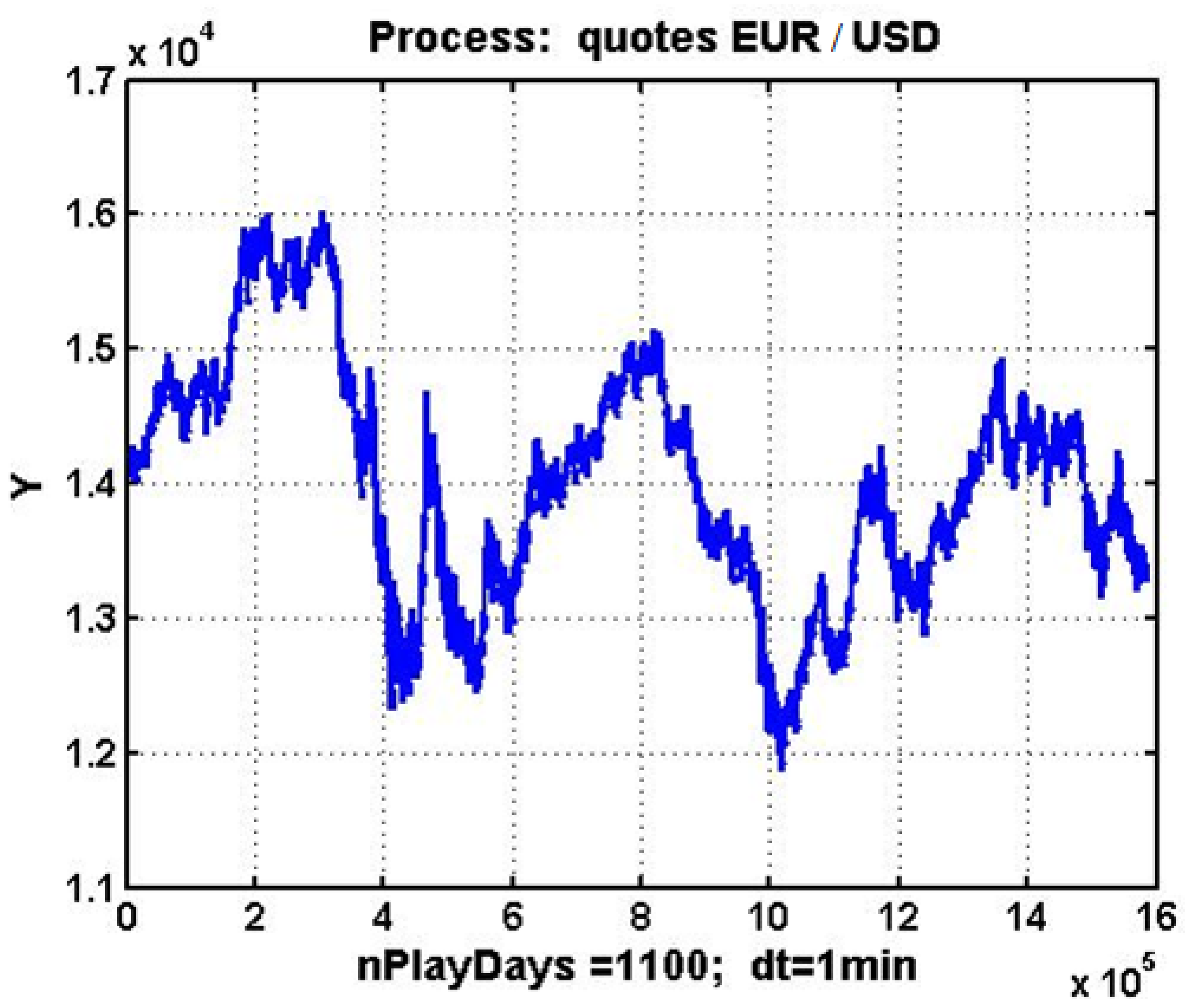
A prime example of a stochastic–chaotic process in action is evident in the fluctuation of the EUR/USD currency pair, for which several empirical studies—employing correlation dimension, largest Lyapunov exponent and BDS–surrogate tests—have documented low-dimensional deterministic chaos (Bildirici & Sonustun, 2019). Although the methodological framework is asset-agnostic, the empirical evaluation in this study is intentionally restricted to the EUR/USD currency pair over a fixed three-year window. High-frequency, one-minute mid-quotes for EUR/USD covering 1 January 2020–31 December 2022 were downloaded from Finam.ru (accessed 12 April 2025). Because the foreign-exchange market operates on a 24 h basis, five days per week, the dataset includes every consecutive minute-stamp across the Asian, European, and North American sessions. Consequently, any generalization to other financial instruments must be confirmed by dedicated case studies and is left for future research.

Figure 1 illustrates the changes in this quotation over a three-year period, with a one-minute discretization. The graph clearly shows that the evolution of quotations is an oscillatory, non-periodic random process, characterized by numerous local trends and distinct signs of self-similarity (Mandelbrot et al., 2004; Crilly et al., 2012). In essence, there is ample reason to posit that the process under scrutiny is an embodiment of stochastic chaos, a notion that has been investigated in the context of econometric data through the lens of market chaos theory (Peters, 1996; A. Musaev et al., 2023a; Gregory Williams & Williams, 2004).

Prices of actively traded instruments are frequently modeled as martingales or, at best, as I(1) processes whose first differences are near-white noise (Fama, 1970). From a risk-management perspective, this implies that shocks have permanent effects on the level series and that the unconditional variance of P_t grows without bound. Forecasting models must therefore (i) operate on transformed data (returns, log-returns), (ii) account for possible cointegration with related macro variables, and (iii) adapt quickly to structural breaks. The ensemble architecture proposed below addresses points (i)–(iii) by combining differenced linear predictors with nonlinear and sentiment-based experts and by dynamically re-weighting them in response to recent forecasting errors.

In light of these considerations, this study introduces a multi-expert forecasting system (MES) that leverages ensemble machine learning algorithms to address the forecasting challenges posed by non-stationary, chaotic financial processes. The EUR/USD currency pair, with its well-documented volatility and complexity (Peters, 1996; Boccaletti et al., 2000), serves as a representative example in our analysis. By integrating diverse forecasting models—each capturing different aspects of market behavior—into a unified decision framework, our proposed MES aims to enhance forecast reliability and thereby improve the quality of risk management decisions.

Despite valuable advances in ensemble forecasting—combining linear, nonlinear and sentiment-based models (e.g., Han et al., 2024; Cretarola et al., 2020)—existing work typically treats bagging, boosting and stacking in isolation and focuses almost exclusively on day-ahead horizons. Moreover, these approaches often lack a supervisory module capable of dynamically adapting expert weights in response to evolving error characteristics under chaotic non-stationarity. As a result, the relative merits of different ensemble strategies across both intraday (one-hour) and day-ahead (24 h) forecasting remain under-examined.

This study fills that gap by developing a two-level MES that unifies diverse weak learners—including polynomial extrapolators, multidimensional regressors and a sentiment expert—within an adaptive stacking framework and by empirically comparing bagging, boosting and stacking on high-frequency EUR/USD data over both one-hour and one-day horizons.

The primary objectives of this research are the following:

i

Elucidate the specific challenges associated with forecasting in chaotic financial environments;

ii

Develop a robust framework for constructing a multi-expert system using ensemble techniques;

iii

Empirically demonstrate the enhanced performance of the proposed system relative to traditional forecasting approaches with a single agent.

Ultimately, this work contributes both to the theoretical understanding of ensemble forecasting in non-stationary settings and to its practical application within financial risk management, offering actionable insights for practitioners operating in volatile markets.

2. Methods

2.1. Observation Model and Problem Statement

A central challenge in forecasting financial and economic time series is their intrinsic chaotic and non-stationary behavior. In many practical scenarios, particularly under volatile market conditions, the observed data cannot be satisfactorily modeled by classical stationary processes. To formally capture this complexity, we represent the observation series $y_k$ as an additive model based on Wold’s decomposition (Wold, 1938),

$$y_k=x_k+v_k,\hspace{1em}k=1,\dots ,\hspace{0.17em}N,$$

(1)

where $x_k$ denotes the unknown deterministic “system” component that encapsulates the regular underlying dynamics of the process, and $v_k$ represents the stochastic noise component associated with measurement errors or external disturbances.

Traditionally, it is assumed that the system component $x_k$ is sufficiently smooth—amenable to representations by polynomial or trigonometric series. However, in environments characterized by instability and rapid regime shifts, the dynamics of $x_k$ often follow an oscillatory, non-periodic pattern typical of deterministic chaos. In these settings, the smoothness assumption is frequently violated.

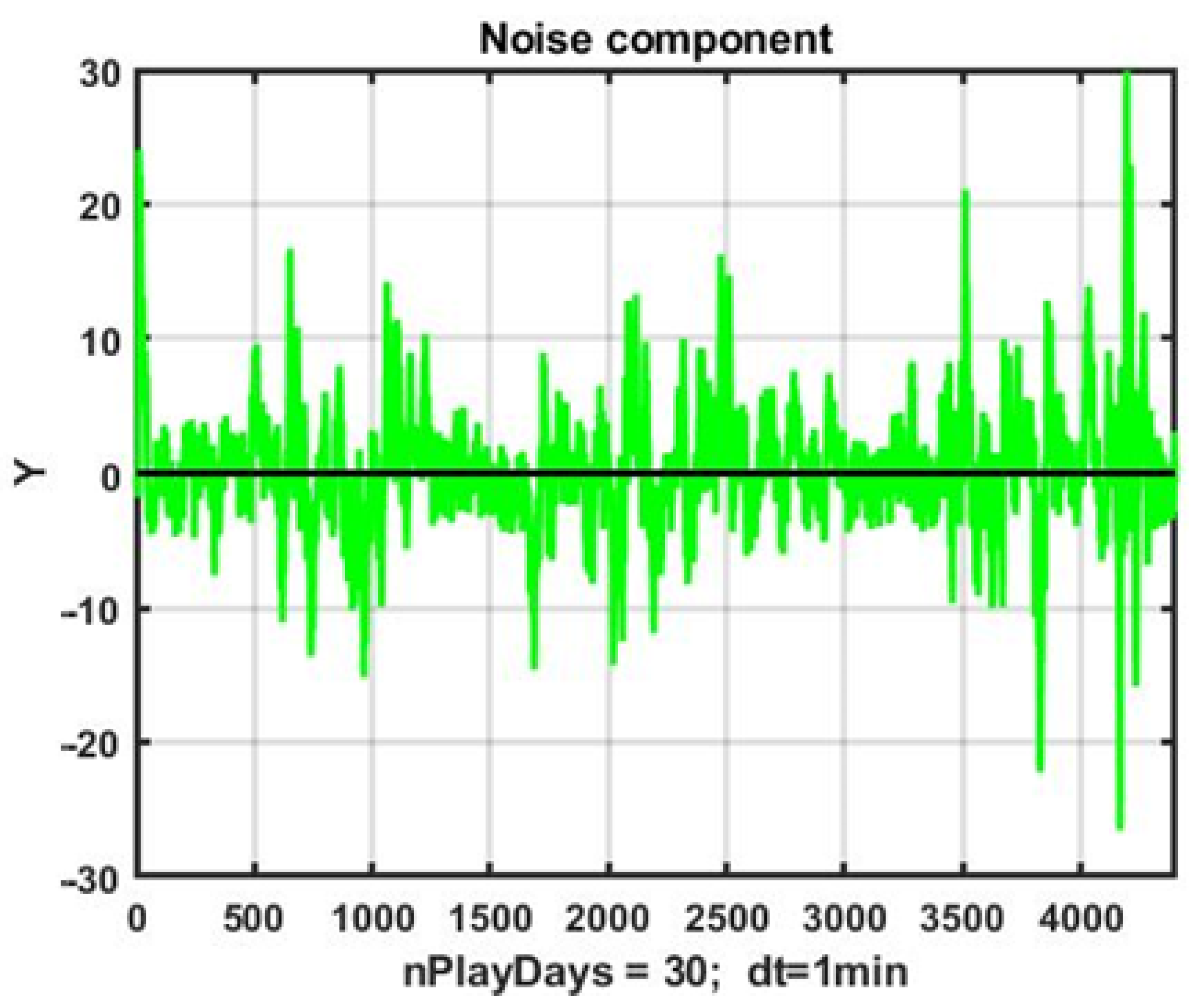
In conventional approaches, the noise component $v_k$ is modeled as Gaussian white noise. Yet, empirical evidence indicates that for many financial time series, the noise is non-stationary and exhibits heteroscedasticity. A more realistic representation involves modeling $v_k$ as a mixture process that converges weakly to a Huber-type Gaussian model,

$$v_k\sim \left(1-\epsilon \right)N\left(0,\hspace{0.17em}{\sigma }_1^2\right)+\epsilon N\left(0,\hspace{0.17em}{\sigma }_2^2\right),\hspace{1em}\epsilon \in \left(0,\hspace{0.17em}1\right),\hspace{1em}{\sigma }_2>>{\sigma }_1,$$

where $\epsilon$ is a fouling coefficient that quantifies the degree of contamination (Huber, 1981). Moreover, for heteroscedastic processes, the noise variance is time-dependent, denoted as $\sigma =\sigma \left(t\right)$.

An illustration of the non-stationary noise component, generated by subtracting a smoothed estimate of $x_k$ (using a transfer coefficient $\alpha =0.05$) from the observation series, is provided in Figure 2.

The transfer coefficient α controls the aggressiveness of the exponential filter: smaller α values yield stronger smoothing and a longer effective time constant T ≈ 1/α. At α = 0.05, the filter effectively averages over the last 20 observations, reducing noise but introducing a lag of approximately τ = (1/α − 1) steps.

The presence of heteroscedasticity and numerous abnormal observations undermines the applicability of traditional identification and forecasting schemes. Even adaptive algorithms are rendered less effective, as they require considerable time to recalibrate tracking contours, thus failing to capture rapid and chaotic changes in the process dynamics.

These challenges motivate the transition to multi-expert systems (MES) (A. Musaev & Grigoriev, 2022). Rather than relying on a singular forecasting model, MES employs a diverse group of software experts (SEs), each characterized by distinct forecasting methodologies and parameterizations. Formally, each expert is defined by a mapping,

$$Exp\left(S,\hspace{0.17em}P\right): \left(Y_{\left(k-T,\hspace{0.17em}k-1\right)},\hspace{0.17em}\hspace{0.17em}{y}_k\right)\to {\tilde{x}}_{k+\tau },\hspace{1em}k=1,\dots ,n,$$

(2)

where $Y_{\left(k-T,\hspace{0.17em}k-1\right)}=\left\{y_{k-T},\hspace{0.17em}{y}_{k-T+1},\dots ,y_{k-1}\right\}$ is the array of historical observations used for training, $y_k$ is the current observation, and ${\tilde{x}}_{k+\tau }$ represents the forecast over a horizon $\tau$. By operating M experts simultaneously or sequentially, a set of candidate forecasts is generated, ${\tilde{X}}_{k+\tau }=\left\{{\tilde{x}}_{k+\tau }\left(i\right),\hspace{1em}i=1,\dots ,M\right\}$, at each forecasting step $k=1,\dots ,n$.

The forecasting task then consists of optimally combining these candidate forecasts. In particular, the goal is to determine the forecast ${\tilde{x}}_k^{*}$ that minimizes a chosen efficiency indicator $Q\left({\tilde{x}}_k,\hspace{0.17em}{x}_k\right)$,

$${\tilde{x}}_k^{*}=extr\hspace{0.17em}Q\left({\tilde{x}}_k,\hspace{0.17em}{x}_k\right),\hspace{1em}k=1,\dots ,n,$$

(3)

where “extr” denotes the extraction of an optimal value according to the performance criterion. For linear computational schemes, the criterion is often defined as the mean squared error (MSE),

$$Q\left({\tilde{x}}_k,\hspace{0.17em}{x}_k\right)={\displaystyle \frac{1}{n}}{\displaystyle \sum }_{k=1}^n{({\tilde{x}}_k-\hspace{0.17em}{x}_k)}^2,$$

(4)

or alternatively, the mean absolute deviation (MAD),

$$Q\left({\tilde{x}}_k,\hspace{0.17em}{x}_k\right)={\displaystyle \frac{1}{n}}{\displaystyle \sum }_{k=1}^n\left|{\tilde{x}}_k-\hspace{0.17em}{x}_k\right|.$$

(5)

Thus, the optimal forecasting problem is formulated as follows:

$${\tilde{x}}_k^{*}=arg\hspace{0.17em}minQ\left({\tilde{x}}_k,\hspace{0.17em}\hspace{0.17em}{x}_k\right)$$

(6)

It is important to note that the forecast itself is not an end but a tool to support superior management decisions. An inherent benefit of employing MES lies in its ability to adapt to the variability in individual expert performance; whereas a singular “ideal” expert is unlikely to exist, the collective intelligence derived from diverse perspectives enhances overall forecast stability and accuracy.

In summary, the observation model encapsulated by Equations (1)–(6) not only reflects the inherent challenges posed by non-stationary, chaotic dynamics but also establishes the motivation for developing a multi-expert ensemble framework. This framework is intended to bridge the gap between theoretical forecasting improvements and practical risk management applications in volatile financial environments.

Throughout the paper the symbol τ denotes the forecast horizon measured in one-minute bars. Two practical horizons are analyzed as follows: (i) τ = 1 440 (~24 h) for the day-ahead trading scenario and (ii) τ = 60 (~1 h) for intraday risk-control experiments. Unless stated otherwise, results in Section 3.3, Section 3.4 and Section 3.5 refer to the latter setting.

2.2. Problem of Smoothing Non-Stationary Observation Series

Extracting the underlying system component $x_k$ from the additive mixture (1) is a challenging task, particularly when dealing with non-stationary and chaotic time series. Conventional dynamic smoothing methods, although necessary, tend to introduce significant bias in the estimated signal. Figure 3 illustrates the effects of filtering the observation series using an exponential smoothing filter (Gardner, 1985) defined as follows:

$${\stackrel{⌢}{x}}_k=\alpha y\left(t\right)+\left(1-\alpha \right){\stackrel{⌢}{x}}_{k-1}={\stackrel{⌢}{x}}_{k-1}+\alpha \left(y_k-{\stackrel{⌢}{x}}_{k-1}\right),\hspace{1em}k=1,\dots ,n,$$

where two different transfer coefficients are considered: a relatively mild smoothing with ${\alpha }_1=0.05$ and a stronger smoothing with ${\alpha }_2=0.0075$.

With the milder setting (${\alpha }_1=0.05$), the filtered series retains numerous stochastic local inflections. This property, while preserving much of the original dynamic detail, can lead to an increased incidence of type II errors—so-called “false alarms” in change detection—where the system erroneously signals a trend change. Conversely, a smaller coefficient (${\alpha }_2=0.0075$) produces a heavily smoothed signal in which the identified breakpoints tend to correspond to significant trend shifts; however, this comes at the cost of an inherent delay due to the offset in the estimated values. Such delays can result in untimely decisions, thereby reducing overall management efficiency.

This trade-off underscores the need for the development of advanced sequential filtering algorithms that can achieve an optimal level of smoothing while minimizing bias and delay. Several alternative approaches have been proposed in the literature (e.g., A. Musaev et al., 2023b) and serve as the basis for the implementation of various software expert (SE) variants within our multi-expert system framework. Below, we briefly describe three such approaches.

2.3. A Polynomial Extrapolator

One of the simplest software expert models is based on polynomial extrapolation. In this approach, a sliding observation window,

$$Y_{\left(k-L,\hspace{0.17em}k\right)}=\left(y_{k-L},\hspace{0.17em}{y}_{k-L+1},\dots ,y_k\right),$$

(7)

is used to capture the local dynamics of the process $y_k.$ The forecasting model is given by a power polynomial of the following form:

$$\hspace{1em}\hspace{0.17em}{x}_p\left(t_j\right)={\displaystyle \sum }_{i=0}^p{a}_i{t}^j,\hspace{1em}j=1,\dots ,L,\hspace{1em}$$

(8)

which acts as a deterministic extrapolator. The model parameters are determined by a vector of optional parameters $P=\left(L,\hspace{0.17em}\alpha ,\hspace{0.17em}p,\hspace{0.17em}\tau \right)$, where L is the size of the sliding window, α is the transfer coefficient used in smoothing, p is the polynomial degree, and τ is the forecasting horizon. According to the Weierstrass approximation theorem (Stone, 1948; Khanh & Quan, 2019), any continuous function can be uniformly approximated by polynomials; however, the rapid dynamics of chaotic processes necessitate the construction of a polynomial model on a window immediately preceding the forecast interval $\left(k+1,\dots ,\hspace{0.17em}k+\tau \right)$, with the parameters $\left({\alpha }_0,\hspace{0.17em}{\alpha }_1,\dots ,\hspace{0.17em}{\alpha }_p\right)$ obtained via least squares minimization,

$${\alpha }^{*}:\hspace{0.17em}\hspace{0.17em}min{{\displaystyle \sum }}_{j=1}^L{(y_j-x_p\left(t_j\right))}^2,$$

(9)

is then produced by substituting the forecast time into the polynomial,

$${\tilde{x}}_{k+c}=x_p\left(k+c\right),\hspace{1em}c=1,\dots ,\tau .$$

(10)

This approach rests on the inertia hypothesis of the observed process. However, as demonstrated in (A. Musaev et al., 2023c), many financial time series lack clear inertial behavior, limiting the applicability of this method. Moreover, increasing the polynomial degree beyond 3–4 can lead to degeneracy in the system of normal equations and may require additional regularization.

2.4. Multidimensional Regression Forecast

For processes exhibiting correlations among multiple variables, a multidimensional regression predictor can offer an effective alternative (Lauritzen, 2023; A. Musaev et al., 2023a, 2023d). The observation model in this context is expressed in the following vector form:

$$Y_k=X_k+V_k$$

(11)

where $Y_k=\left\{y_{k,j}=x_{kj}+v_{k,j},\hspace{1em}j=1,\dots ,\hspace{0.17em}m\right\},\hspace{1em}k=1,\dots ,\hspace{0.17em}n$.

A training data matrix is constructed over a sliding window of length L, where the regressors are time-shifted by the forecasting interval $\tau$,

$$Y_{\left(L,m\right)}=\left\{y_{k-L-\tau ,j},\hspace{0.17em}\dots ,y_{k-\tau ,j},\hspace{1em}k=1,\dots ,\hspace{0.17em}L,\hspace{0.17em}\hspace{0.17em}j=1,\dots ,\hspace{0.17em}m\right\}.$$

(12)

In the case of forecasting a single process using m-1 correlated processes, the regression model is formulated as follows:

$$Y_k=C_k{Y}_{\left(k-L,k\right)}+V_k,$$

(13)

where $C_k={(c_1,\dots ,c_m)}_k^T$ represents the coefficients defining a hyperplane in m-dimensional space, and $Y_{\left(k-L,k\right)}$ is composed of shifted observations,

$$Y_{\left(k-L,k\right)}=\left[\begin{array}{cccc}1& y_{1,k-L}& \dots & y_{m,k-L}\\ 1& y_{1.k-L+1}& \dots & y_{m.k-L+1}\\ \dots & \dots & \dots & \dots \\ 1& y_{1,k}& \dots & y_{m,k}\end{array}\right], V={(v_1,\dots ,v_m)}^T ,$$

(14)

Standard regression assumptions apply, such as zero mean of the noise components and independence among them,

$$E\left\{V_j\right\}=0;\hspace{0.17em}\hspace{0.17em}E\left\{Y_{k,j},\hspace{0.17em}{V}_{kj}\right\}=0, cov\left(V_i,\hspace{0.17em}{V}_j\right)=,\{\begin{array}{c}0,\hspace{1em}i\ne j\\ {\sigma }^2,\hspace{1em}i=j\end{array} ,\forall i,j=1,\dots ,m.$$

(15)

By minimizing the sum of squared errors $V^{T}V={(Y_k-Y_{\left(k-L,k\right)}{C}_k)}^T\left(Y_k-Y_{\left(k-L,k\right)}{C}_k\right)$, we come to a system of normal equations, the solution of which is determined by a well-known relationship, ${\stackrel{⌢}{C}}_k={(Y_{\left(k-L,k\right)}^T{Y}_{\left(k-L,k\right)})}^{-1}{Y}_{\left(k-L,k\right)}{Y}_k$. The time shift by τ ensures that the obtained regression coefficients ${\stackrel{⌢}{C}}_k$ serve as a suitable linear predictive operator for the SE.

2.5. Precedent Forecast

The precedent forecasting approach is based on the assumption that similar historical patterns yield similar future outcomes—a concept aligned with human cognitive judgment of similarity (Fukunaga, 2013). In practice, this method involves scanning the historical data using a sliding window,

$$Y_{\left(i,\hspace{0.17em}i+L-1\right)}=\left(y_i,\dots ,y_{i+L-1}\right),\hspace{1em}i=1,\dots ,\hspace{0.17em}{N}_S-L,$$

(16)

where $N_S$ denotes the size of the historical training set. During the scanning process, the algorithm identifies $M_a$ analog windows (denoted by their indices $i_1^{*},,\dots ,i_{M_a}^{*}$) that minimize a chosen similarity metric—typically the root mean square error (4) or the mean absolute deviation (5)—when compared to the current observation window,

$$Y_{\left(k,\hspace{0.17em}k-L+1\right)}=\left(y_{k-L+1},\dots ,y_k\right),\hspace{1em}k=L+1,\dots ,\hspace{0.17em}n.$$

The scanning window with the smallest metric value is considered as a precedent. As measures of similarity between windows $Y_{k+L+1,\hspace{0.17em}k}$ and $Y_{i,\hspace{0.17em}i+L-1},\hspace{1em}i=1,\dots ,\hspace{0.17em}{N}_S-L$ in machine learning tasks, distances of the type of root mean square deviation (4) or mean absolute deviations (5) are usually used.

The following remarks have been made:

• When computing metrics, it is recommended to use centered data values in observation windows (15). Furthermore, in instances of significant heteroscedasticity of the observed process, it is advisable to normalize the data in the state and scanning windows by estimates of their standard deviations (std).
• The size of the observation window L is typically selected based on the minimization of the total square error, which encompasses the sum of the variance and the square of the bias induced by dynamic errors. However, this approach is not suitable for chaotic environments due to the non-stationarity of observation series. In such cases, the size of the state window L should be viewed as a parameter to be refined during the process of model adaptation.
• For certain tasks aimed at estimating the local trend, the difference between the coefficients of linear approximation ${\alpha }_1$ of observation series in the current state and scanning windows can serve as a measure of similarity,

  $${\rho }_i\left[y_C,\hspace{0.17em}{y}_S\right]={\alpha }_1\left(y_c\left(k\right)\right)-{\alpha }_1\left(y_S\left(i\right)\right),\hspace{1em}i=1,\dots ,N_S-L.$$

As a forecast, as already noted, the smoothed aftermath is used, following the precedent window ${\tilde{x}}_{k+1,k+\tau }=x_{i^{*}+L+1,\hspace{0.17em}{i}^{*}+L+\tau }$, i.e., immediately after the scanning window with the minimum value of the chosen metric,

$$i*:\hspace{0.17em}\hspace{0.17em}{\rho }_{i^{*}}\left[y_C,\hspace{0.17em}{y}_S\right]=\min ,\hspace{1em}\forall i=1,\dots ,N_S-L.$$

(17)

The transition to the forecast of the systemic component (1) ${\tilde{y}}_{k+1,k+\tau }\to {\tilde{x}}_{k+1,\hspace{0.17em}k+\tau }$ can be made by sequentially smoothing the result of the forecast, for example, using an exponential filter.

2.6. Limits of Traditional Forecasting Under Unit Root Non-Stationarity and Chaotic Regimes

Empirical log price series for liquid FX pairs such as EUR/USD are well documented to possess a unit root: the level P_t is integrated of order one (I(1)), whereas the first difference ΔP_t (the return) is usually weakly stationary with near-zero linear autocorrelation, in line with the weak-form Efficient-Markets Hypothesis (Fama, 1970; Phillips & Perron, 1988).

The random walk representation P_t = P_t−1 + u_t immediately induces high sample autocorrelation in the level series, although the shocks u_t themselves are serially uncorrelated. Thus, non-stationarity stems from the permanent impact of shocks, not from the mere fact that P_t is a stochastic process. Ignoring this distinction leads to spurious regressions and invalidates estimators whose consistency relies on repeated samples from an identical distribution. Any forecasting scheme that does not difference, cointegrate, or otherwise neutralize the unit root implicitly assumes repeatability of mean and variance and is therefore prone to systematic bias.

Beyond unit root behavior, high-frequency currency data exhibit signatures of deterministic chaos: small perturbations in initial conditions produce widely diverging paths (Bildirici & Sonustun, 2019). Two data windows that appear almost identical under Euclidean metrics can evolve in strikingly different ways a few minutes later. This lack of local repeatability explains why purely similarity-based techniques from classical technical analysis often fail and motivates the use of an ensemble of weak, heterogenous learners whose weights adapt to local error dynamics.

The crux of this issue lies in the failure of the essential assumption of repeatability under identical conditions. In chaotic environments, even slight random fluctuations can instigate radical shifts in the dynamic behavior of the series. This volatility implies that data segments, which appear nearly identical when assessed via standard similarity metrics, may nonetheless diverge dramatically in their subsequent evolution. Such unpredictability partly explains the limited effectiveness of traditional technical analysis (Iskrich & Grigoriev, 2017; Escher, 2019; Parameswaran, 2022) in guiding trading operations in capital markets.

To quantify the performance of individual Software Expert (SE) predictors in trading tasks, their effectiveness is defined as the ratio between the number of successful forecasts $m_i^{+}$ (i.e., those where the prediction’s direction aligns with the actual market move) and the total number of forecasts m_i for the i-th predictor,

$$h_i^{+}=m_i^{+}/m_i,\hspace{1em}i=1,\dots ,M_e.$$

(18)

A more precise evaluation of trading efficiency (Yusupov et al., 2021) is obtained by estimating the net gain realized from implementing a management strategy S. This gain is defined as follows:

$$R\left(S\right)={{\displaystyle \sum }}_{j=1}^m\Delta y_j={{\displaystyle \sum }}_{j=1}^m{y}_j\left(k_{close}\right)-y_j\left(k_{open}\right).$$

(19)

Here, $\Delta y_j=y_j\left(k_{close}\right)-y_j\left(k_{open}\right)$, $j=1,\dots ,m$, represents the outcome of the j-th trade, calculated as the difference between the asset value at the closing $\left(k_{close}\right)$ and opening ($k_{open}$) of the position, with m being the total number of operations performed. The sign of the difference $\Delta y_j,\hspace{1em}j=1,\dots ,m$ is determined by the condition of coincidence or discrepancy of the directions of the forecast and the real dynamics of the process on the forecasting interval.

To benchmark the proposed experts, we also employ the classical persistence model. For price levels, this is the random walk assumption ${\stackrel{⌢}{P}}_{t+\mathsf{\tau }}=P_t$, while for log-returns it degenerates to ${\stackrel{⌢}{r}}_{t+1}=0$, i.e., the best mean-square forecast is “no change”. In the trading framework that follows, a directional signal is therefore taken as follows:

$$d_{t+1}^{RW}=sign\left(P_t-P_{t-1}\right),$$

which corresponds to the directional-persistence rule, “tomorrow will move in the same direction as today”. Because this rule needs no parameters and uses only the last observation, it represents the minimal-information baseline recommended by (Armstrong, 2001) and is commonly required by forecasting guidelines.

3. Experiments

From the three-year master dataset, we extracted a 100-day estimation window for parameter fitting. For graphical illustration in Figure 4, Figure 5, Figure 6, Figure 7 and Figure 8, we further selected a 10-day subset that spans both trending and range-bound regimes. We chose this particular subset because it covers diverse market situations—like clear trends and periods where the market moves sideways—which makes it ideal for thoroughly testing our strategies.

3.1. A Software Expert Based on Linear Extrapolation

To establish a baseline for forecasting in daily Forex trading, we implement a software expert that employs a first-order linear extrapolation. In this approach, the training phase uses a sliding observation window of duration L = 1440 min (i.e., one full calendar day). Within each window, the observed time series is modeled by a first-order polynomial, $x_j=a_0+a_{1}j,\hspace{1em}j=1,\dots ,L,$ where the coefficients $\left(a_0,\hspace{0.17em}{a}_1\right)$ are estimated using the least squares minimization (LSM) as described in (9). The forecast for the next day (that is, 1440 one-minute observations)—spanning a forecast horizon τ = L—is produced by directly substituting the corresponding time indices into the fitted polynomial, that is, ${\tilde{x}}_{k+c}=x_p\left(k+c\right),\hspace{1em}c=1,\dots ,\tau$.

As an initial diagnostic, we applied the Augmented Dickey–Fuller test to the level series; the test failed to reject the unit root null (ADF p-value = 0.74), confirming the I(1) behavior discussed in Section 2.6. Consequently, all forecasts were generated either in the log-return domain or with model specifications that explicitly accommodate integrated processes. The length of the rolling estimation window L was re-optimized each day so that it constituted the shortest span yielding coefficient estimates that remained statistically stable at the conventional 5% significance threshold.

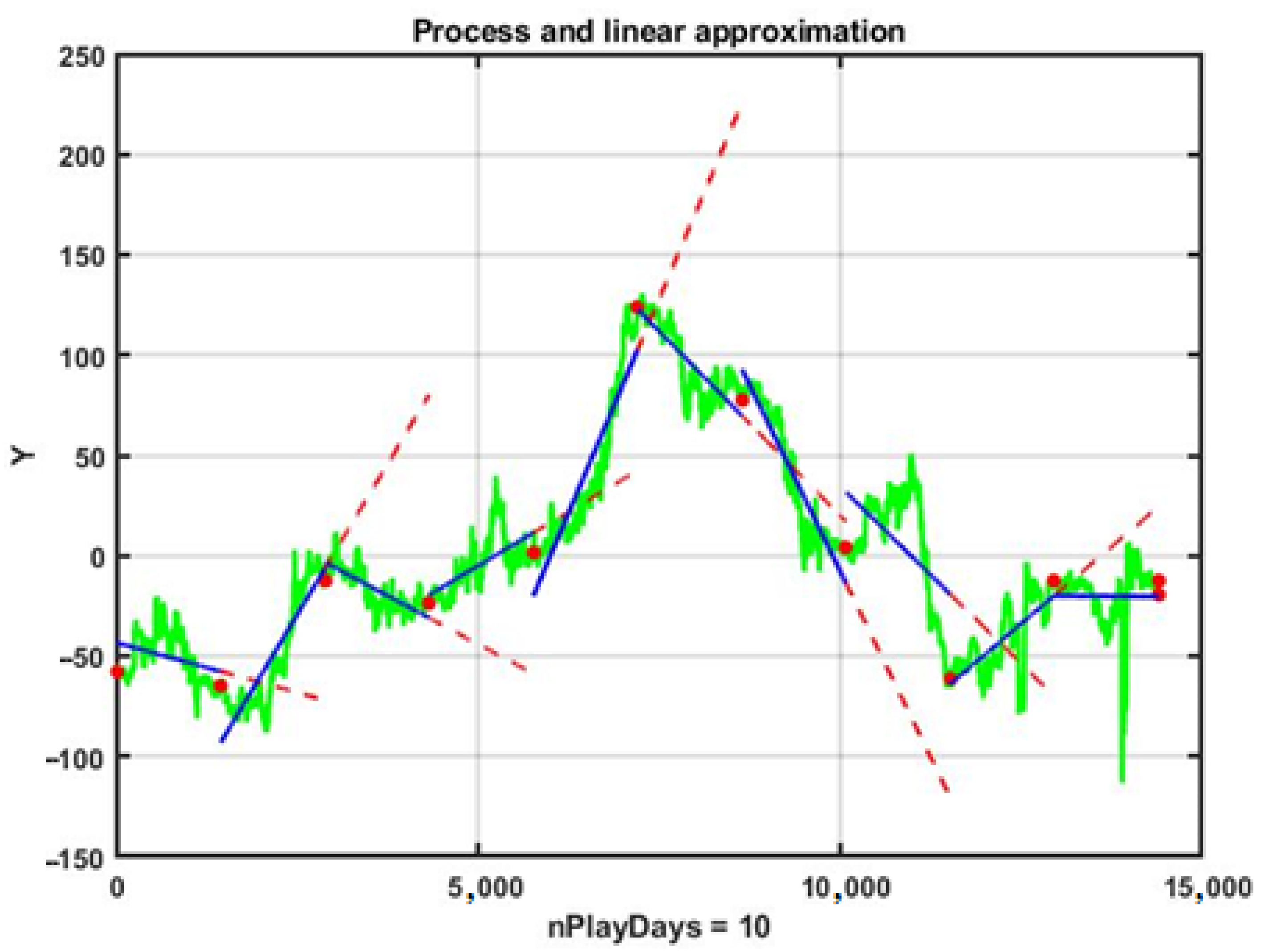
Figure 4 illustrates this process using centered EUR/USD quotes over a 10-day period. In the figure, the boundaries of the daily observation intervals are marked by red dots. The blue solid lines represent the linear approximations obtained on each day’s data, while the red lines depict the linear forecasts generated by naturally extending these trends into the next day. It is evident from Figure 4 that only three out of nine observation intervals resulted in forecasts whose trend directions were aligned with the actual market movement, yielding an estimated probability of favorable outcomes $F^{+}\approx 0.33$ (see also metric (18)).

Recognizing that the 10-day interval was selected primarily for illustrative clarity, we extended the experiment to a 100-day observation period to enhance statistical reliability. In this case, the success rate improved only modestly to $F^{+}\approx 0.40$, while the cumulative performance metric (as defined in (19)) indicated a net loss of −210 points. These results clearly highlight that the simple linear extrapolator functions as a “weak learner” in the machine learning context—it fails to independently generate forecasts of adequate quality for effective management decisions under chaotic market conditions.

Motivated by this limitation, the remainder of this study investigates the potential of MES technology to integrate diverse forecasting approaches and thereby enhance overall prediction accuracy, as outlined in (A. Musaev & Grigoriev, 2022).

3.2. Constructing a Two-Level MES Using Ensemble Machine Learning Methods

In this study, a two-level MES is developed to enhance forecasting performance in chaotic financial environments. At the lower level, a set of $M_e$ software experts (SEs) is employed; these experts differ either in the structure or in the parameters of their forecasting algorithms. The second level is formed by a Software Expert–Supervisor (SE-S) that processes the local decisions of the individual experts and generates the final forecast, which ultimately informs the management decision.

The simplest aggregation method implemented by SE-S is the unweighted averaging of the forecasts from the individual SEs. Mathematically, if ${\tilde{x}}_{k,k+\tau }$ represents the forecast from the k-th expert for future time $k+\tau$, then the combined forecast is given by the following:

$${\tilde{x}}_{k,k+\tau }={\displaystyle \frac{1}{M_e}}{{\displaystyle \sum }}_{i=1}^{M_e}{x}_t^i,\hspace{1em}t=k+1,\dots ,k+\tau ,\hspace{1em}k=1,\dots ,n,$$

(20)

which provides a baseline ensemble prediction. A more refined approach relies on weighted averaging, where each expert’s forecast is weighted inversely with respect to an a priori estimation of its Bayesian risk. Specifically, after sequentially solving the forecasting task for each SE using the retrospective database $Y_S$, the average forecasting error $\delta {\tilde{X}}_{k,\tau }^i$ is computed and the corresponding Bayesian risk $r_{k,i}^{\tau }$ is estimated. The final forecast is then defined as follows:

$${\tilde{x}}_{t+\tau }={{\displaystyle \sum }}_{i=1}^{M_e}{w}_i{\tilde{x}}_{t+\tau }^i/{{\displaystyle \sum }}_{i=1}^{M_e}{w}_i, w_i={(r_i^{\tau })}^{-1}, i=1,\dots ,m, t=k+1,\dots ,\hspace{0.17em}\tau .$$

(21)

In practice, the actual management decision is determined by this final forecast along with an experimentally selected critical threshold $\delta {(x_k)}^{*}={({\tilde{x}}_k-x_k)}^{*}$.

A fundamental challenge in constructing an MES is that, under the conditions of chaotic dynamics, each SE typically acts as a “weak learner.” To overcome this limitation, ensemble machine learning techniques—namely bagging, boosting, and stacking—are incorporated. In these frameworks, the supervisor acts as a meta-learner to enhance the overall forecast reliability relative to individual SE outputs.

3.3. Ensemble Forecast for Chaotic Process Based on Bagging Technology

Bagging (Bootstrap Aggregating) relies on generating multiple training subsets from the original dataset to train a homogeneous set of SEs. Each expert in this approach is identical in structure but is trained on different resampled or sliding subsets of data. In non-stationary environments, however, the empirical distribution of the data changes over time, and so relying on bootstrap resampling can be less effective. To address this issue, this work proposes the use of sliding window samples of different lengths, taken immediately prior to the forecast time. Increasing the sample length improves the quality of smoothing and reduces the probability of Type II errors (false alarms), albeit at the cost of increased Type I errors (delays in change detection).

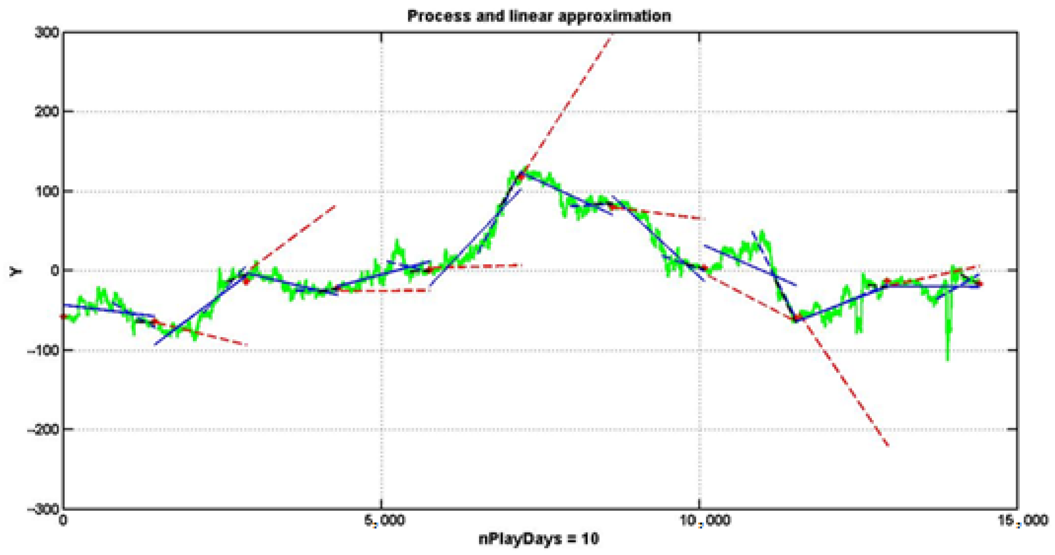
For example, consider a bagging framework applied to a linear extrapolation forecast in a daily trading scenario. Three variants are used, each employing training windows of different lengths: $L=1440$ min counts (1 day), $L_1=720$ counts and $L_2=360$ counts. These intervals are positioned directly adjacent to the forecast starting point, and the forecast is carried out on a daily interval ($\tau =1440$ counts). As shown in Figure 5, the learning outcomes of the three SE extrapolators are displayed as linear approximations (solid blue, blue dashed, and black dashed lines), and the final forecast for each trading day is based on the averaged least squares estimates of the coefficients,

$${\tilde{x}}_{k+i}=a_o+a_{1}t,\hspace{1em}t=1,\dots ,\tau ,$$

(22)

where $a_o=\left(a_{o1}+a_{o2}+a_{o3}\right)/3,\hspace{1em}{a}_1=\left(a_{11}+a_{12}+a_{13}\right)/3$.

Although simple bagging based on linear extrapolators may not yield highly effective forecasts under conditions of inertialess market chaos, the approach shows more promise when applied to processes with inherent inertia (see A. Musaev et al., 2023c). It is important to note that the example presented is intended for illustration only; real-world trading strategies require dynamic entry points rather than static daily divisions.

3.4. Ensemble Forecast for a Chaotic Process Based on Boosting Technology

Boosting improves forecast accuracy by sequentially correcting the errors of homogeneous models. In the context of forecasting, boosting involves updating the weights of individual forecasts based on their errors, thereby refining the overall weighted average forecast. In our approach, the boosting algorithm operates on the basis of precedent data analysis: a sliding observation window,

$$Y_{\left(k,\hspace{0.17em}k-L+1\right)}=\left(y_{k-L+1},\dots ,y_k\right),\hspace{1em}k=L+1,\dots ,\hspace{0.17em}n,$$

(23)

is defined for the current state, and similar historical observation windows are identified from a retrospective database.

A set of indices $i_1^{*},,\dots ,i_{M_a}^{*}$ corresponding to the smallest values of a chosen similarity metric is selected. The most similar window, having the minimum similarity value ${\mu }_1=\min (Y_{k,\hspace{0.17em}k-L+1},\hspace{1em}{Y}_{i,\hspace{0.17em}i+L-1}),\hspace{1em}\forall i=1,\dots ,\hspace{0.17em}{N}_S-L,$ is assigned a unit weight $w_1=1$. Other windows are assigned weights relative to ${\mu }_1$ by $w_{i_e}={\mu }_{i_e}/{\mu }_1,\hspace{1em}\forall i_e=1,\dots ,\hspace{0.17em}{M}_e$. The final forecast is then obtained as a weighted average of the forecast consequences of the identified analog windows,

$${\tilde{x}}_{\left(k+1,\hspace{0.17em}k+\tau \right)}={{\displaystyle \sum }}_{j=1}^{M_e}{w}_{i_j^{*}}{y}_{i_j^{*}+L+1,\hspace{0.17em}{i}_j^{*}+L+\tau }/{{\displaystyle \sum }}_{j=1}^{M_e}{w}_{i_j^{*}}.$$

(24)

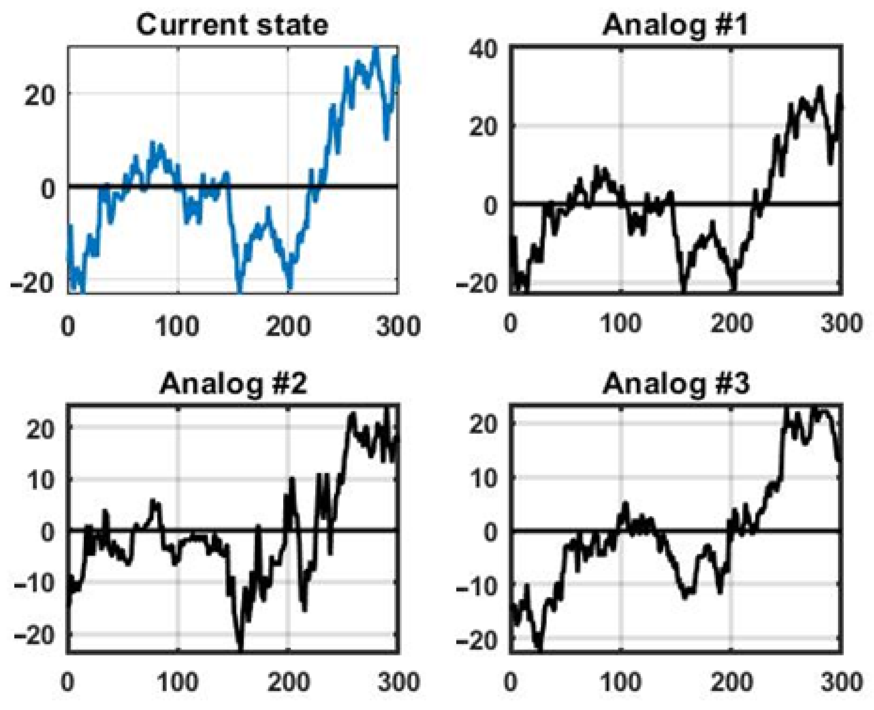
As a numerical example, consider precedent forecasting for the EUR/USD currency pair using a sliding window of length L = 300 counts, with a scanning window from retrospective data shifted by 150 counts. The training dataset spans 300 days of continuous monitoring with a 1 min time discretization. At each step, a similarity metric—such as the mean absolute difference—is evaluated, and Figure 6 illustrates the current state window (blue graph) alongside three analogous windows extracted from the historical database.

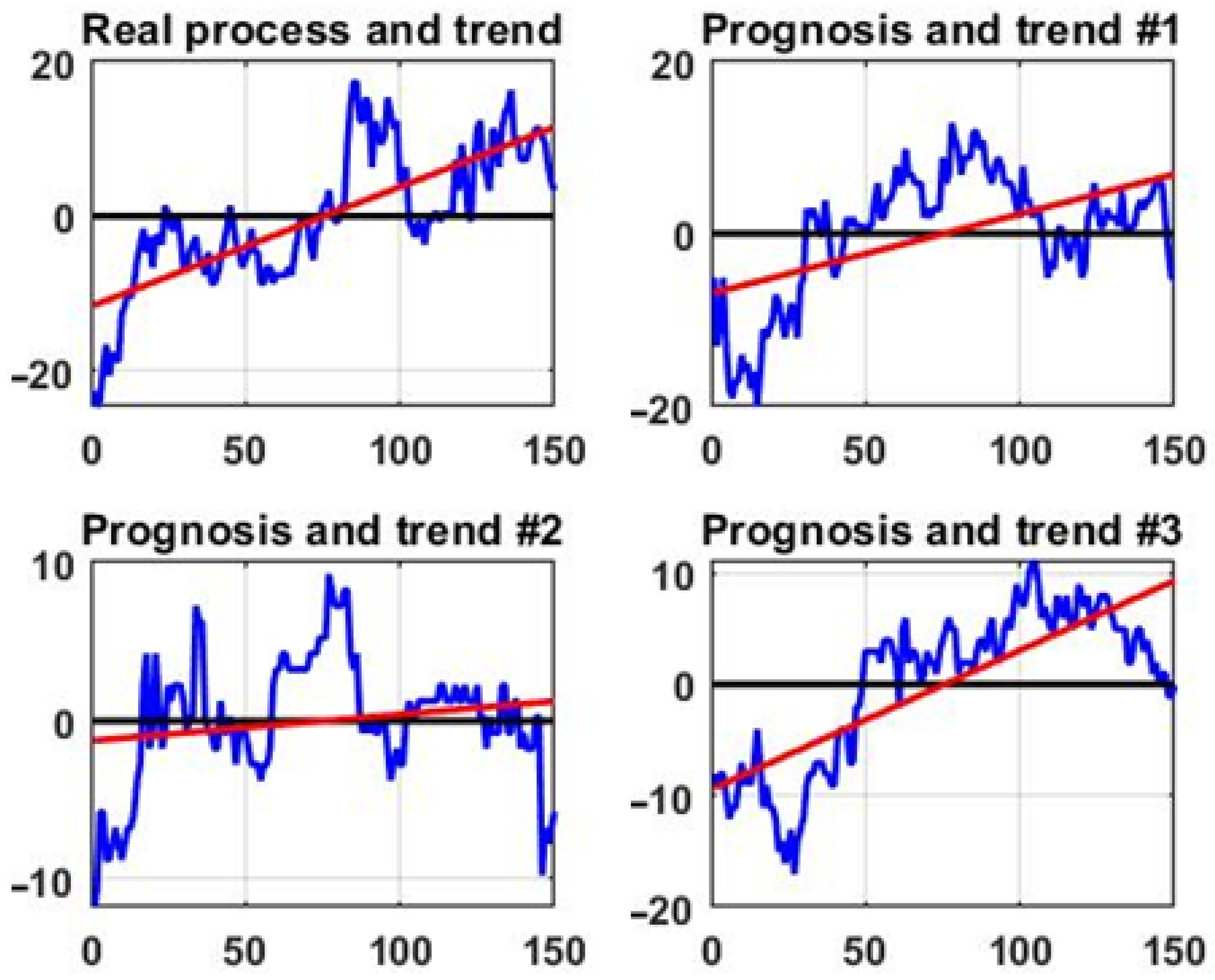
Figure 7 then shows the corresponding forecast outcomes and the linear trends (red lines) estimated via least squares. Although the boosting algorithm successfully predicts the trend direction across several forecast windows, its performance may vary over the entire observation period due to the inherently unpredictable nature of market chaos.

3.5. Ensemble Forecast for a Chaotic Process Based on Stacking Technology

Stacking involves the integration of heterogeneous forecasting algorithms—each considered a “weak learner”—to produce a more reliable final forecast. In our stacking approach, each SE independently generates a prediction for the same forecast interval τ, and the supervisory expert (SE-S) subsequently acts as a meta-learner to combine these predictions.

The outputs of the individual experts are formulated as fuzzy decisions drawn from the set,

$$D=\left\{1,\hspace{0.17em}0,\hspace{0.17em}-1\right\},$$

(25)

where +1 indicates an upward trend, −1 indicates a downward trend, and 0 represents a flat or sideways trend. The final decision is determined by a threshold condition, for example,

$$d=\{\begin{array}{c}1,\hspace{1em}\hspace{0.17em}\alpha >{\alpha }^{*},\\ 0,\hspace{1em}\hspace{0.17em}\left|\alpha \right|<{\alpha }^{*},\\ -1,\hspace{1em}\hspace{0.17em}\alpha <-{\alpha }^{*},\end{array}$$

(26)

with $\alpha$ representing the coefficient of linear approximation on the current observation segment and ${\alpha }^{*}$ determined via hypothesis testing (using, for instance, t-distribution tables with L-2 degrees of freedom) (Van Der Waerden, 2013).

In our illustrative implementation, three heterogeneous SEs are used as follows:

• SE-1 employs a linear forecasting algorithm (as per Equation (10)) based on the trend extrapolation from the previous one-day observation window.
• SE-2 is based on regression analysis; its forecasting operator is expressed as follows:

  $${\stackrel{⌢}{x}}_{k+r}={\stackrel{⌢}{C}}_{k,r}{Y}_{Rk},\hspace{1em}k=L,\dots ,n,$$

  (27)

  where ${\stackrel{⌢}{\mathrm{C}}}_{k,r}={({Y_{R<\left(k-L+1\right):\left(k-r-1\right)>}}^T{Y}_{R<\left(k-L+1\right):\left(k-r-1\right)>})}^{-1}{Y_{R[<(k-L+1:\left(k-1\right)>]}}^T{y}_{<k-L+r+1):\left(k-1\right)>}$ is the least squares estimate of the transfer coefficient of the linear filter, and $Y_{Rk}={(y_{R1},\hspace{0.17em}{y}_{R2},\hspace{0.17em}\dots ,y_{Rm})}_k$ is a vector of regressors corresponding to financial instruments strongly correlated with the target asset. Owing to non-stationarity, this forecast is often unstable; thus, an indicative forecast is formed based on the discrepancy between the current multiregression estimate ${\stackrel{⌢}{x}}_k={\stackrel{⌢}{C}}_k{Y}_{Rk},\hspace{1em}k=L,\dots ,n$ and the observed price $x_k=\alpha y_k+\left(1-\alpha \right) x_{k-1}$,$k=2,\dots ,n$. This discrepancy, defined as follows:

  $$d_k={\stackrel{⌢}{x}}_k-x_k,\hspace{1em}k=1,\dots n,$$

  (28)

  is interpreted in light of market mispricing.
• SE-3 utilizes text mining techniques to analyze market sentiment from analytical reviews. The objective is to convert qualitative textual information into a fuzzy decision drawn from D (see Hassani et al., 2020; Liu et al., 2021).

The supervisory expert (SE-S) aggregates the fuzzy outputs from SE-1, SE-2, and SE-3. In an illustrative day-trading simulation using EUR/USD real quotes over a 10-day period, the observation interval is divided into 10 segments (each of 1440 min counts). For all bagging experiments, we adopt an intraday horizon of τ = 60 one-minute bars. At the beginning of each segment, each SE produces a fuzzy decision. These decisions are visually represented by colored arrows in Figure 8: a green arrow for d = +1 (forecasted growth), a red arrow for d = −1 (forecasted decline), and a black two-sided arrow for d = 0 (no significant trend).

The final decision is determined via simple majority voting,

$$d_s=\{\begin{array}{c}1, if {\displaystyle \sum }_{i=1}^3{d}_i>0 \\ -1, if {\displaystyle \sum }_{i=1}^3{d}_i<0 \\ 0, if {\displaystyle \sum }_{i=1}^3{d}_i=0\end{array},$$

(29)

and can alternatively be computed using weighted majority voting if historical accuracy rates $w_i=h_i^{+}, i=1,\dots ,M_e$ for each SE are available,

$$d_s=\{\begin{array}{c}1, if {\displaystyle \sum }_{i=1}^{M_e}{w}_i{d}_i>0 \\ -1, if {\displaystyle \sum }_{i=1}^{M_e}{w}_i{d}_i<0 \\ 0, if {\displaystyle \sum }_{i=1}^{M_e}{w}_i{d}_i=0\end{array}.$$

(30)

The final decision, as aggregated by SE-S, is depicted in Figure 8 by an arrow whose direction and color correspond to the ultimate market entry signal.

4. Results and Discussion

This section presents the empirical evaluation of the proposed ensemble decision-making framework, which integrates heterogeneous software experts (SEs) via stacking techniques over a 100-day observation interval. Over the 100-day evaluation period (144,000 one-minute bars), the study produced 99 day-ahead forecasts and 142,560 intraday one-hour-ahead forecasts, resulting in 142,659 individual point forecasts that underpin the trading and accuracy statistics reported below. The results are analyzed both from a performance perspective—in terms of trading profitability and forecasting accuracy—and with regard to the probabilistic reliability of the ensemble approach under conditions of stochastic chaos.

Table 1. Comparison of trading results for SE and MES. The averages are calculated over M_SE1 = 334 (SE-1), M_SE2 = 100 (SE-2), M_SE3 = 100 (SE-3) and M_MES = 100 (ensemble) realized trades generated during the 100-day evaluation period.

Decisions	Result in Pips.	Probability of Winning	Average Win	Average Loss
RW	−185	0.49	56.2	−57.5
SE-1	−218	0.49	55.6	−54.7
SE-2	1096	0.59	62.7	−63.5
SE-3	788	0.56	59.5	−57.8
MES	1392	0.61	60.1	−58.3

includes the naïve random walk (RW) benchmark alongside the three single-expert (SE) variants and the multi-expert system (MES) that combines their signals by simple majority voting as formalized in Equation (29). The RW rule opens exactly one position per day by repeating the sign of the previous day’s return; over the 100-day evaluation window, this produces 100 trades, a modest loss of −185 pips, and a 49% hit rate. All three SE models meet or modestly surpass this baseline: SE-1 still posts a loss, whereas SE-2 and SE-3 generate positive net results. MES outperforms every individual expert and the RW benchmark, delivering a profit of 1392 pips—1577 pips more than RW and 296 pips above the best SE (SE-2)—while lifting the win probability (Equation (18)) to 61%.

These outcomes demonstrate that aggregating heterogeneous experts provides an economically and statistically meaningful edge over both the minimal-information persistence model and the standalone SEs. Moreover, applying sequential evolutionary optimization procedures (Katoch et al., 2021; A. Musaev et al., 2022; Albadr et al., 2020) to adapt expert weights can boost the MES win probability by an additional 5–8%, further reinforcing the advantage of the proposed framework.

These results indicate that leveraging an ensemble of weak predictors via MES can yield superior trading performance compared to the independent use of individual SEs. The enhanced performance is attributed to the aggregation of diverse, weak forecasting signals, which collectively contribute to forming a more robust management decision.

A fundamental requirement for the practical application of MES is that each individual SE must exceed a 50 percent threshold in the probability of successful decisions. To illustrate this, we consider a binary decision scenario in which a group of $M_e$ experts makes a collective forecast. In this context, the final decision is determined by majority voting, where the necessary vote threshold is given by,

$$m^{+}=\lfloor M_e/2\rfloor +1,$$

with $\lfloor x\rfloor$ denoting rounding x to the nearest smaller integer. Assuming each expert makes an erroneous decision with probability $p$, the overall probability of an erroneous decision by the ensemble is computed using the Bernoulli formula as follows:

$$P_{err}={{\displaystyle \sum }}_{i=1}^{m^{+}}{C}_{M_e}^i{p}^i{(1-p)}^{M_e-i}.$$

(31)

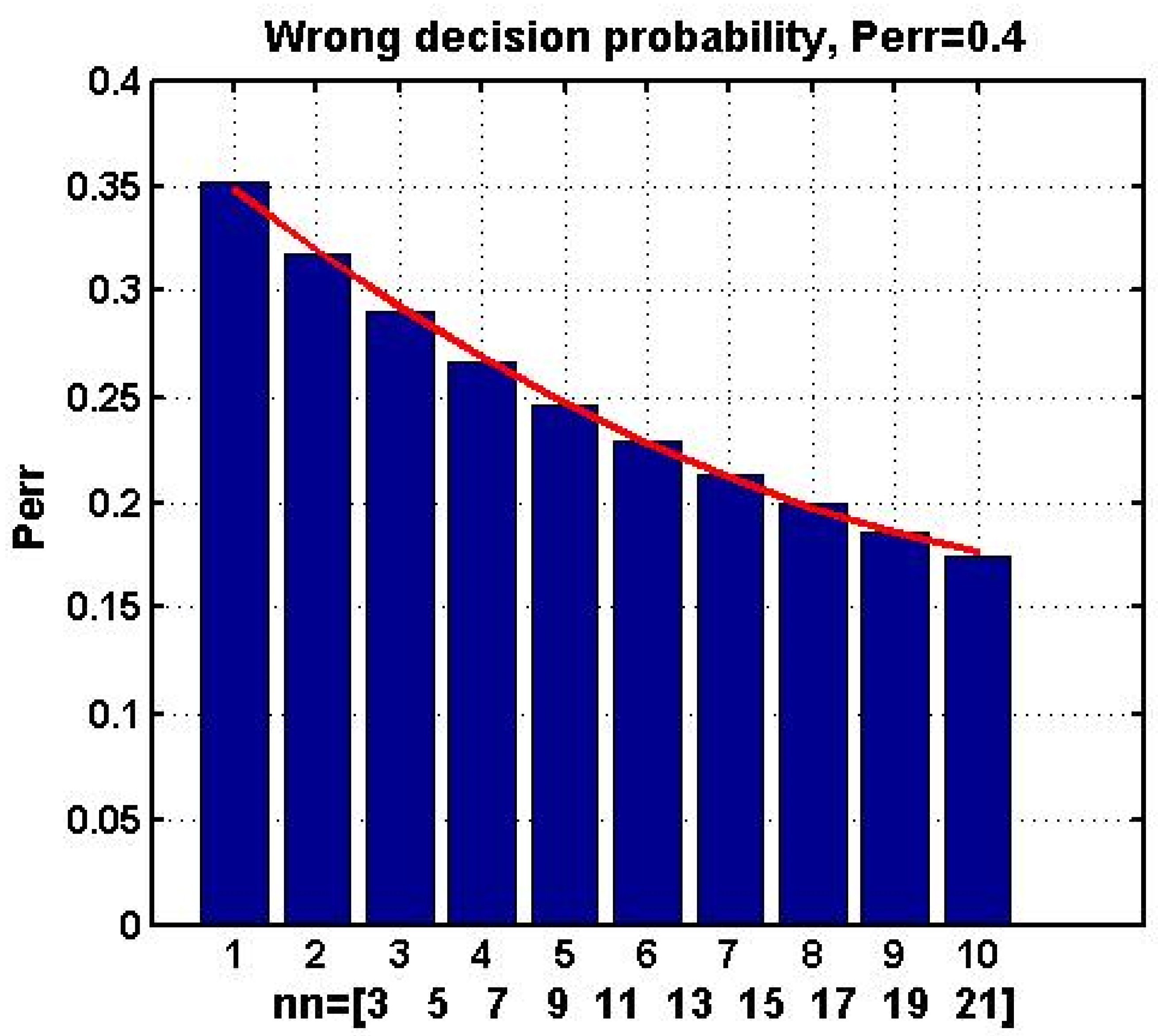
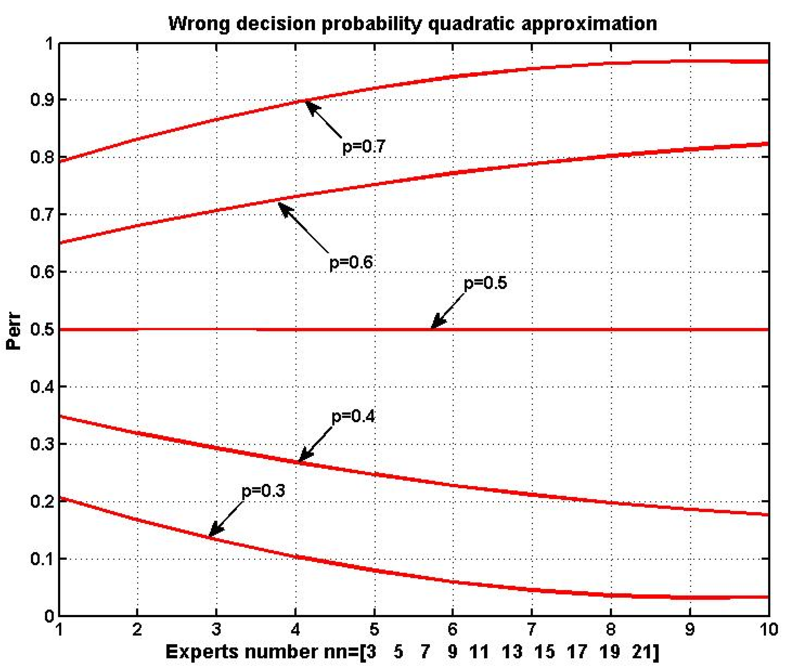
For instance, if p = 0.4, then as the number of experts increases (using odd numbers = 3, 5, …, 21), the probability of an erroneous ensemble decision decreases. Figure 9 illustrates this trend with a bar chart where a red line represents the least squares fit of a second-degree polynomial. A similar trend is observed in Figure 10, which shows polynomial approximations for ensemble error probabilities under different assumed values of p. These figures demonstrate that maintaining an individual expert error probability below p^* = 0.5 is a critical condition for the successful application of MES.

The empirical results clearly suggest that an ensemble approach, which aggregates weak signals from multiple SEs, can significantly improve forecast reliability and trading performance in environments characterized by stochastic chaos. However, it is important to note the following limitations:

• The chaotic nature of financial time series implies that even an SE that exhibits high efficiency during one observation segment may fail under altered market conditions in the subsequent period. This poses challenges in dynamically estimating the individual p-values and assigning appropriate weightings.
• While statistical or adaptive methods for decision fusion remain valuable, their efficiency can be compromised in turbulent regimes where traditional assumptions of stability do not hold (as in the Wald model described by Equation (1)). Similar challenges arise when employing neural networks, which require extensive training to reliably capture chaotic dynamics.
• Despite promising aggregate results, the example presented here does not constitute a guarantee of consistent advantage under all market conditions. Given the inherent uncertainty in chaotic environments, practitioners should use MES as one part of a broader risk management framework, continuously monitored and adjusted using updated market data and retrospective analyses.

5. Conclusions

This study has demonstrated that an ensemble approach, specifically the multi-expert system (MES), can substantially enhance forecasting accuracy and decision-making in unstable environments characterized by stochastic chaos. The improved performance, however, is contingent upon individual software experts (SEs) maintaining a success probability exceeding 50%. This finding underscores the critical importance of integrating multiple weak predictors to offset individual deficiencies—a strategy that ultimately leads to more reliable and robust risk management decisions.

Our empirical results illustrate that while the basic implementations of individual SEs and the MES framework serve well to explain the underlying concepts, further enhancements can be achieved by developing more robust variants of these experts (Maronna et al., 2006; Schmidbauer et al., 2014; A. Musaev et al., 2023e). It is important to note that increasing the stability of a forecasting system by reducing its sensitivity to variations in dynamic and statistical characteristics may come at the cost of overall management efficiency. Therefore, a careful balance must be struck between robustness and agility, particularly in environments where permissible decision boundaries are inherently narrow and dynamic.

The proposed MES framework also opens avenues for the incorporation of advanced aggregation technologies beyond simple majority voting. Emerging techniques based on conflict resolution and compromise (Antipova & Rashkovskiy, 2023; Vinyamata, 2010) offer promising alternatives for integrating diverse expert opinions, potentially leading to even more refined decision-making processes. As illustrated in earlier sections (see Figure 5, Figure 6, Figure 7 and Figure 8), these sophisticated mechanisms may significantly improve the operational performance of the system when applied to real-world financial scenarios.

Mansurov et al. (2023) support the idea that integrating adaptive, self-learning components into multi-expert systems not only mitigates individual model deficiencies but also aligns aggregate forecasts more closely with observed market behavior. Such insights provide a compelling rationale for employing ensemble machine learning techniques that aggregate diverse forecasting methodologies to improve risk management and decision-making in volatile financial environments.

In practical terms, the ensemble approach detailed herein provides risk managers and financial practitioners with a promising tool for navigating the challenges of volatile markets. Future research should focus on the following:

(i)

Refining the robustness of individual SEs within the MES framework;

(ii)

Exploring alternative decision aggregation methods that can dynamically adapt to market changes;

(iii)

Validating the methodology on a broader spectrum of financial datasets to enhance its practical applicability.

Ultimately, this work contributes to the ongoing discourse on managing uncertainty and risk in financial markets by offering a viable path toward improved forecast reliability and decision-making effectiveness.