3.1. Cumulative Abnormal Returns Analysis—2020 and 2024 Halving Events
Initially, linear regressions were performed using the ordinary least squares method on data regarding the price of Bitcoin and the 365-day moving average values during both analysis periods.
Figure 1 illustrates the relationship between Bitcoin’s closing price and its 365-day moving average during the reference interval for the 2020 halving event. This comparison establishes a baseline for price behavior before the halving, which is essential when modeling normal returns.
As shown in
Figure 1, the closing price closely follows the moving average, suggesting consistent market conditions in the reference period, in contrast to the fluctuations observed during the event window.
Figure 2 depicts the relationship between Bitcoin’s closing price and its 365-day moving average during the event interval for the 2020 halving. This figure is crucial for identifying deviations from normal price behavior around the halving event.
In
Figure 2, the widening gap between the closing price and the moving average reflects the market’s reaction to the halving, exacerbated by external factors such as the COVID-19 pandemic.
Figure 3 shows the relationship between Bitcoin’s closing price and its 365-day moving average during the reference interval for the 2024 halving event. This serves as a benchmark for normal market conditions prior to the 2024 halving.
As illustrated in
Figure 3, the price tracks the moving average closely, indicating that the market was relatively stable in the months leading up to the 2024 halving.
Figure 4 presents the relationship between Bitcoin’s closing price and its 365-day moving average during the event interval for the 2024 halving. This figure highlights the market’s response to the halving event in a more mature market environment.
The coefficients of determination (
R2) of the regression models showed significant differences in both years, with a value of 0.70 for the reference interval and 0.37 for the period of events in 2024, as well as 0,27 and 0,05 in 2020. This indicates a variation in the representativeness of the linear model between the intervals evaluated. An analysis of the significance of the parameters of the linear models used was conducted, with the following results, and both models presented statistically significant parameters at a 95% confidence level (
p-value = 0).
Table 1 summarizes key economic parameters for Bitcoin during the reference and event periods of the 2020 and 2024 halving events. These metrics, including average daily return and volatility, reveal how market dynamics shift around the halving.
Table 2 provides a detailed comparison of Bitcoin’s economic parameters before and after the 2020 and 2024 halving events. This breakdown allows for a closer examination of how the market adjusted in the immediate lead-up and aftermath of each halving.
We observed higher average returns during the pre-halving periods of both events. The minimum returns exhibited similar levels; however, regarding maximum returns, it is noteworthy that, in March 2020, at the onset of the COVID-19 pandemic, there was a significant impact on the asset’s performance, resulting in a negative return of 47.99% in a single day. This led to an average volatility of 5% and triggered a drawdown that extended over 158 days. Following the recovery from the event, in the post-halving period, the return and volatility values across both periods converged once again.
The correlation between the volatility curves is presented in
Table 3.
The volatility correlations in
Table 3 indicate varying dynamics between 2020 and 2024. The weak positive correlation (0.547) in the 60-day pre-halving window suggests some alignment in volatility patterns, possibly due to shared market expectations. The strong negative correlation (−0.843) in the 14-day post-halving window for 2020 reflects the pandemic’s disruptive impact, contrasting with 2024’s more stable post-halving period (0.624 in the 240-day window), indicating improved investor adaptation and market efficiency.
Figure 5 compares the 30-day volatility of Bitcoin during the reference and event periods for the 2020 and 2024 halvings. This figure is essential for understanding how market risk changes around these events.
As seen in
Figure 5, volatility peaked significantly during the 2020 event period, likely influenced by the pandemic, while the 2024 event shows a more moderate increase, suggesting greater market resilience.
To evaluate the correlation between the asset’s closing price and volatility during the event period, the correlation coefficient between these two variables was calculated. The obtained values were −0.71 for 2020 and 0.30 for 2024, indicating a weak positive correlation between the closing price and the asset’s volatility in 2024, but a stronger negative correlation in 2020, possibly due to the destabilizing effect of the pandemic.
Figure 6 plots Bitcoin’s closing price against its 30-day volatility during the event interval for the 2020 halving. This figure helps visualize the relationship between price movements and market risk during the halving period.
Figure 7 displays Bitcoin’s closing price and 30-day volatility during the event interval for the 2024 halving. This figure reveals how price and volatility interact in a more stable market environment.
In contrast to 2020,
Figure 7 shows a weaker relationship between price and volatility in 2024, indicating that the market was less reactive to price changes during this halving.
The negative correlation (−0.71) between price and volatility in 2020, as shown in
Figure 6, underscores the market’s sensitivity to external shocks during this period.
For both intervals studied, abnormal returns were obtained by calculating the difference between the daily continuous return of the actual prices and the daily continuous return obtained through the respective regression equation. The cumulative abnormal return (CAR), representing the sum of the returns over the evaluated periods, was then calculated.
Figure 8 tracks the cumulative abnormal returns (CARs) for Bitcoin during the 2020 halving event.
As illustrated in
Figure 8, the CAR reached its highest point just before the halving but dropped significantly during the event window, reflecting the market’s initial optimism and subsequent correction.
Figure 9 presents the cumulative abnormal returns (CARs) for Bitcoin during the 2024 halving event. This figure highlights the market’s more muted response compared to earlier cycles.
In
Figure 9, CAR peaks earlier and returns to baseline faster than in 2020, indicating that the market anticipated the halving’s impact more effectively in 2024.
An analysis of the abnormal returns during the 2020 and 2024 halvings showed similarities and differences. The pandemic caused significant losses starting in March 2020; however, these were slowly recovered over time, with positive cumulative returns seen at the end of the post-halving period. This pandemic impact might have disrupted typical return dynamics, possibly preventing much higher gains, especially since positive cumulative returns were recorded early in the pre-halving window before the big drop. In 2024, there were no major disruptive events, and some stabilizing factors helped, such as the hope for better market rules, more money coming from ETFs by big financial firms, and countries like El Salvador planning to hold cryptocurrency reserves. These factors likely led to a significant increase in the maximum level of cumulative positive abnormal returns.
It is interesting to note that in both halving events we examined, by the end of the 240-day window, the cumulative return values between the reference and event periods came closer together. This suggests that changes in mining currency supply might not affect asset returns as much as market expectations do, and that mining costs tend to follow the asset’s price movements rather than predict them, which matches the findings obtained by (
Ramos et al., 2021). Despite the reduced currency supply post-halving, the expected sustained increase in cumulative abnormal returns did not occur, indicating that external factors may have had a stronger influence than supply-side effects.
3.2. Return and Volatility Analysis—2012 to 2024 Halvings
In this section, the asset’s behavior was evaluated in terms of its return and volatility during pre- and post-halving periods, using time windows of 240 days (long-term), 30 days (medium-term), and 7 days (short-term). The behavior of Bitcoin during these periods was studied, considering all halving events that have already occurred, as presented in
Table 4.
The mean return and volatility were calculated for all halving periods, considering different time windows. This approach aimed to capture, in a more precise and direct manner, the effects related to the halving of the profitability and risk associated with the asset, both in the short and long term. The inclusion of all periods in the analysis also sought to identify trends in returns and volatility over the years, as Bitcoin has gradually undergone changes in its investor profile and regulatory framework, resulting in increased adoption in the investment portfolios of various sizes worldwide. These changes could lead to greater maturity of the asset, potentially reducing its volatility and, consequently, the returns it provides over time.
The data pertaining to the mean return are presented in
Table 5.
Figure 10 illustrates the mean daily returns across all halving events.
In 2012, we see the highest returns at 0.23%, 0.76%, and 0.92% for the short, medium, and long windows, which makes sense given the early market’s high volatility and growth.
But the trend goes down from there—by 2024, returns are much lower, with a negative −0.23% in the 30-day window, hinting that the market is maturing and becoming less volatile. The graph backs this up, showing a sharp drop from 2012 to 2016, somewhat of a bounce back in 2020 (probably due to the post-pandemic recovery), and then a leveling off at lower values in 2024, especially in the shorter windows. This suggests that as Bitcoin becomes more widely used and regulated, the effect of halving on returns becomes weaker, probably because market expectations and outside factors play a bigger role now.
The data obtained for the average volatility during the periods are presented in
Table 6.
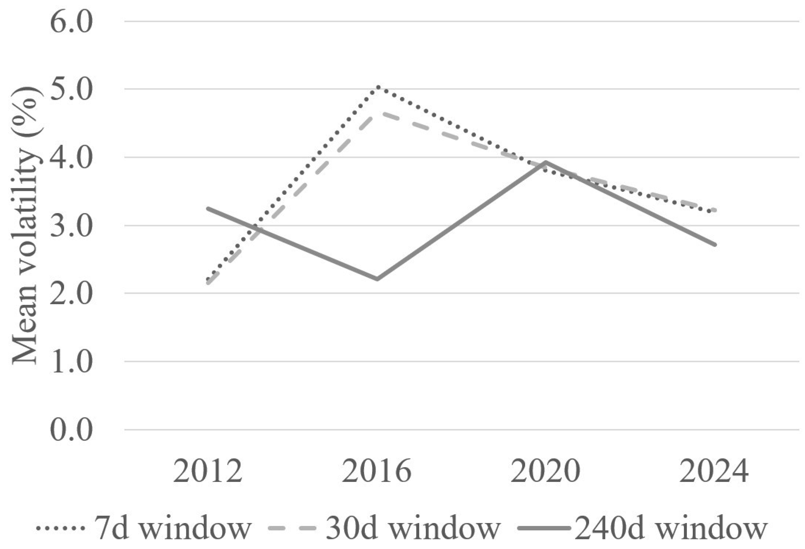
The illustrative graph of the mean volatility is presented in
Figure 11.
Figure 11 reveals different volatility patterns across the four halving cycles. For the 7-day and 30-day windows, volatility peaked in 2016 at 5.04% and 4.67%, respectively, before declining to 3.19% and 3.22% in 2024. In the 240-day window, volatility was highest in 2020 at 3.92%, influenced by the COVID-19 pandemic, but dropped to 2.72% in 2024, indicating greater market resilience and efficiency in pricing predictable supply shocks.
The lower volatility in 2024 (2.72%) compared to 2012 (3.24%) and 2020 (3.92%) suggests increasing market efficiency, as investors better price in predictable supply reductions, reducing the scope for speculative overreactions. The gradual decline after the peaks may reflect market stabilization or reduced speculative activity.
Figure 6 visually supports these findings, showing how different time windows capture unique aspects of Bitcoin’s market behavior during halving cycles.


 ,
, 


