
Exploratory Dividend Optimization with Entropy Regularization


Abstract
1. Introduction
2. Problem
2.1. The Model
2.2. Classical Optimal Dividend Problem
2.3. Exploratory Formulation
- (i)
- for any , where is a set of probability density functions with support ;
- (ii)
- The stochastic differential Equation (9) has a unique solution under π;
- (iii)
- .
3. Exploratory HJB Equation
3.1. Exploratory Dividend Policy
3.2. Verification Theorem
3.3. Solution to Exploratory HJB
- (i)
- If , is nonincreasing.
- (ii)
- If , is nondecreasing.
- (iii)
- If , .
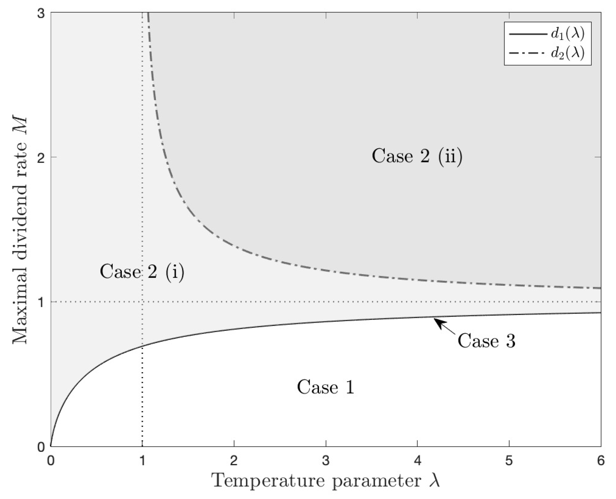
4. Discussion
- (a)
- DefineThen, is increasing. Therefore, and ;
- (b)
- DefineThen, , and is decreasing on . Therefore, and .
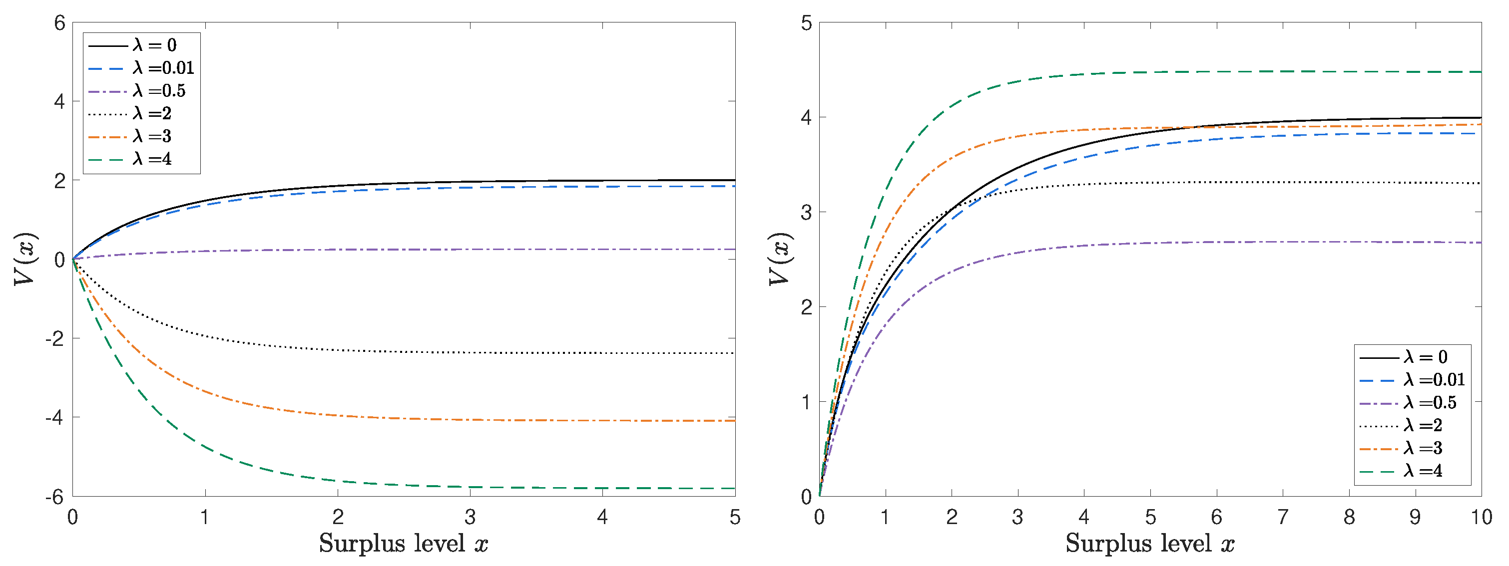
5. Numerical Examples
6. Conclusions
Author Contributions
Funding
Data Availability Statement
Conflicts of Interest
Appendix A. Proof
- (i)
- is continuous and decreasing in x;
- (ii)
- There exists a unique such that ;
- (iii)
- , for some constant , which depends on k only;
- (iv)
- , .
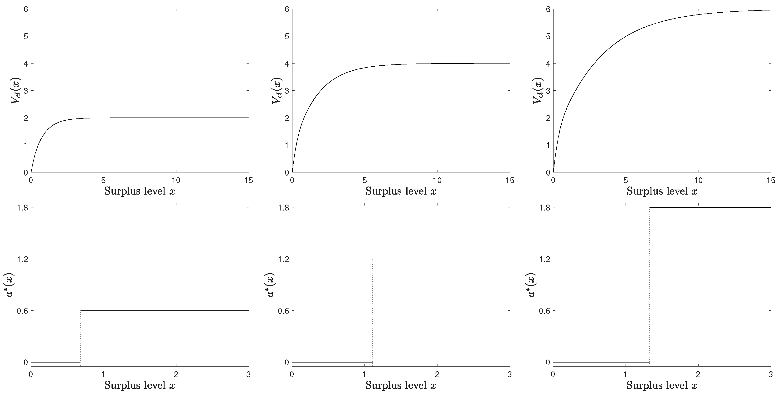
| 1 | For example, the dividend-paying rate under the threshold strategy is the maximal rate if the surplus exceeds the threshold; otherwise, it pays nothing. Because the threshold is determined by the model parameters, the change in the estimated parameters may dramatically change the dividend-paying rate from zero to the maximal rate, or vice versa. |
| 2 | |
| 3 | For each initial surplus x, we discretize the continuous time into small pieces () and sample 2000 independent surplus processes to simulate and . |
References
- Asmussen, Søren, and Michael Taksar. 1997. Controlled diffusion models for optimal dividend pay-out. Insurance: Mathematics and Economics 20: 1–15. [Google Scholar] [CrossRef]
- Asmussen, Søren, Bjarne Højgaard, and Michael Taksar. 2000. Optimal risk control and dividend distribution policies. example of excess-of loss reinsurance for an insurance corporation. Finance and Stochastics 4: 299–324. [Google Scholar] [CrossRef]
- Auer, Peter, Nicolo Cesa-Bianchi, and Paul Fischer. 2002. Finite-time analysis of the multiarmed bandit problem. Machine learning 47: 235–56. [Google Scholar] [CrossRef]
- Avram, Florin, Zbigniew Palmowski, and Martijn R. Pistorius. 2007. On the optimal dividend problem for a spectrally negative lévy process. The Annals of Applied Probability 17: 156–80. [Google Scholar] [CrossRef]
- Azcue, Pablo, and Nora Muler. 2005. Optimal reinsurance and dividend distribution policies in the cramér-lundberg model. Mathematical Finance: An International Journal of Mathematics, Statistics and Financial Economics 15: 261–308. [Google Scholar] [CrossRef]
- Azcue, Pablo, and Nora Muler. 2010. Optimal investment policy and dividend payment strategy in an insurance company. The Annals of Applied Probability 20: 1253–302. [Google Scholar] [CrossRef]
- Bai, Lihua, Thejani Gamage, Jin Ma, and Pengxu Xie. 2023. Reinforcement learning for optimal dividend problem under diffusion model. arXiv arXiv:2309.10242. [Google Scholar]
- Cesa-Bianchi, Nicolò, Claudio Gentile, Gábor Lugosi, and Gergely Neu. 2017. Boltzmann exploration done right. Advances in Neural Information Processing Systems 30. [Google Scholar]
- Choulli, Tahir, Michael Taksar, and Xun Yu Zhou. 2003. A diffusion model for optimal dividend distribution for a company with constraints on risk control. SIAM Journal on Control and Optimization 41: 1946–79. [Google Scholar] [CrossRef]
- Dai, Min, Yuchao Dong, and Yanwei Jia. 2023. Learning equilibrium mean-variance strategy. Mathematical Finance 33: 1166–212. [Google Scholar] [CrossRef]
- De Finetti, Bruno. 1957. Su un’impostazione alternativa della teoria collettiva del rischio. In Transactions of the XVth International Congress of Actuaries. New York: International Congress of Actuaries, vol. 2, pp. 433–43. [Google Scholar]
- Gaier, Johanna, Peter Grandits, and Walter Schachermayer. 2003. Asymptotic ruin probabilities and optimal investment. The Annals of Applied Probability 13: 1054–76. [Google Scholar] [CrossRef]
- Gao, Xuefeng, Zuo Quan Xu, and Xun Yu Zhou. 2022. State-dependent temperature control for langevin diffusions. SIAM Journal on Control and Optimization 60: 1250–68. [Google Scholar] [CrossRef]
- Gerber, Hans U. 1969. Entscheidungskriterien für den zusammengesetzten Poisson-Prozess. Ph.D. thesis, ETH Zurich, Zürich, Switzerland. [Google Scholar]
- Gerber, Hans U., and Elias S. W. Shiu. 2006. On optimal dividend strategies in the compound poisson model. North American Actuarial Journal 10: 76–93. [Google Scholar] [CrossRef]
- Jaderberg, Max, Wojciech M Czarnecki, Iain Dunning, Luke Marris, Guy Lever, Antonio Garcia Castaneda, Charles Beattie, Neil C. Rabinowitz, Ari S. Morcos, Avraham Ruderman, and et al. 2019. Human-level performance in 3d multiplayer games with population-based reinforcement learning. Science 364: 859–65. [Google Scholar] [CrossRef] [PubMed]
- Jeanblanc-Picqué, Monique, and Albert Nikolaevich Shiryaev. 1995. Optimization of the flow of dividends. Uspekhi Matematicheskikh Nauk 50: 25–46. [Google Scholar] [CrossRef]
- Jgaard, Bjarne Hø, and Michael Taksar. 1999. Controlling risk exposure and dividends payout schemes: Insurance company example. Mathematical Finance 9: 153–82. [Google Scholar] [CrossRef]
- Komorowski, Matthieu, Leo A. Celi, Omar Badawi, Anthony C. Gordon, and A. Aldo Faisal. 2018. The artificial intelligence clinician learns optimal treatment strategies for sepsis in intensive care. Nature Medicine 24: 1716–20. [Google Scholar] [CrossRef] [PubMed]
- Kulenko, Natalie, and Hanspeter Schmidli. 2008. Optimal dividend strategies in a cramér–lundberg model with capital injections. Insurance: Mathematics and Economics 43: 270–78. [Google Scholar] [CrossRef]
- Lundberg, Filip. 1903. Approximerad framställning af sannolikhetsfunktionen. Återförsäkring af kollektivrisker. Akademisk afhandling. Stockholm: Almqvist & Wiksells. [Google Scholar]
- Mirowski, Piotr, Razvan Pascanu, Fabio Viola, Hubert Soyer, Andrew J. Ballard, Andrea Banino, Misha Denil, Ross Goroshin, Laurent Sifre, Koray Kavukcuoglu, and et al. 2016. Learning to navigate in complex environments. arXiv arXiv:1611.03673. [Google Scholar]
- Mnih, Volodymyr, Koray Kavukcuoglu, David Silver, Andrei A. Rusu, Joel Veness, Marc G. Bellemare, Alex Graves, Martin Riedmiller, Andreas K. Fidjeland, Georg Ostrovski, and et al. 2015. Human-level control through deep reinforcement learning. Nature 518: 529–33. [Google Scholar] [CrossRef]
- Nachum, Ofir, Mohammad Norouzi, Kelvin Xu, and Dale Schuurmans. 2017. Bridging the gap between value and policy based reinforcement learning. Advances in Neural Information Processing Systems 30. [Google Scholar]
- Paulus, Romain, Caiming Xiong, and Richard Socher. 2017. A deep reinforced model for abstractive summarization. arXiv arXiv:1705.04304. [Google Scholar]
- Radford, Alec, Rafal Jozefowicz, and Ilya Sutskever. 2017. Learning to generate reviews and discovering sentiment. arXiv arXiv:1704.01444. [Google Scholar]
- Schmidli, Hanspeter. 2007. Stochastic Control in Insurance. Cham: Springer Science & Business Media. [Google Scholar]
- Silver, David, Aja Huang, Chris J. Maddison, Arthur Guez, Laurent Sifre, George Van Den Driessche, Julian Schrittwieser, Ioannis Antonoglou, Veda Panneershelvam, Marc Lanctot, and et al. 2016. Mastering the game of go with deep neural networks and tree search. Nature 529: 484–89. [Google Scholar] [CrossRef] [PubMed]
- Silver, David, Julian Schrittwieser, Karen Simonyan, Ioannis Antonoglou, Aja Huang, Arthur Guez, Thomas Hubert, Lucas Baker, Matthew Lai, Adrian Bolton, and et al. 2017. Mastering the game of go without human knowledge. Nature 550: 354–59. [Google Scholar] [CrossRef] [PubMed]
- Strulovici, Bruno, and Martin Szydlowski. 2015. On the smoothness of value functions and the existence of optimal strategies in diffusion models. Journal of Economic Theory 159: 1016–55. [Google Scholar] [CrossRef]
- Tang, Wenpin, Yuming Paul Zhang, and Xun Yu Zhou. 2022. Exploratory hjb equations and their convergence. SIAM Journal on Control and Optimization 60: 3191–216. [Google Scholar] [CrossRef]
- Todorov, Emanuel. 2006. Linearly-solvable markov decision problems. Advances in Neural Information Processing Systems 19. [Google Scholar]
- Wang, Haoran, and Xun Yu Zhou. 2020. Continuous-time mean–variance portfolio selection: A reinforcement learning framework. Mathematical Finance 30: 1273–308. [Google Scholar] [CrossRef]
- Wang, Haoran, Thaleia Zariphopoulou, and Xun Yu Zhou. 2020. Reinforcement learning in continuous time and space: A stochastic control approach. Journal of Machine Learning Research 21: 1–34. [Google Scholar]
- Yang, Hailiang, and Lihong Zhang. 2005. Optimal investment for insurer with jump-diffusion risk process. Insurance: Mathematics and Economics 37: 615–34. [Google Scholar] [CrossRef]
- Yin, Chuancun, and Yuzhen Wen. 2013. Optimal dividend problem with a terminal value for spectrally positive levy processes. Insurance: Mathematics and Economics 53: 769–73. [Google Scholar] [CrossRef]
- Zhao, Yufan, Michael R. Kosorok, and Donglin Zeng. 2009. Reinforcement learning design for cancer clinical trials. Statistics in Medicine 28: 3294–315. [Google Scholar] [CrossRef] [PubMed]
- Zhu, Yuke, Roozbeh Mottaghi, Eric Kolve, Joseph J. Lim, Abhinav Gupta, Li Fei-Fei, and Ali Farhadi. 2017. Target-driven visual navigation in indoor scenes using deep reinforcement learning. Paper presented at 2017 IEEE International Conference on Robotics and Automation (ICRA), Singapore, May 29–June 3; pp. 3357–64. [Google Scholar]
- Ziebart, Brian D., Andrew L. Maas, J. Andrew Bagnell, and Anind K. Dey. 2008. Maximum entropy inverse reinforcement learning. Paper presented at AAAI, Chicago, IL, USA, July 13–17, vol. 8, pp. 1433–38. [Google Scholar]

Disclaimer/Publisher’s Note: The statements, opinions and data contained in all publications are solely those of the individual author(s) and contributor(s) and not of MDPI and/or the editor(s). MDPI and/or the editor(s) disclaim responsibility for any injury to people or property resulting from any ideas, methods, instructions or products referred to in the content. |
© 2024 by the authors. Licensee MDPI, Basel, Switzerland. This article is an open access article distributed under the terms and conditions of the Creative Commons Attribution (CC BY) license (https://creativecommons.org/licenses/by/4.0/).
Share and Cite
Hu, S.; Zhou, Z. Exploratory Dividend Optimization with Entropy Regularization. J. Risk Financial Manag. 2024, 17, 25. https://doi.org/10.3390/jrfm17010025
Hu S, Zhou Z. Exploratory Dividend Optimization with Entropy Regularization. Journal of Risk and Financial Management. 2024; 17(1):25. https://doi.org/10.3390/jrfm17010025
Chicago/Turabian StyleHu, Sang, and Zihan Zhou. 2024. "Exploratory Dividend Optimization with Entropy Regularization" Journal of Risk and Financial Management 17, no. 1: 25. https://doi.org/10.3390/jrfm17010025
APA StyleHu, S., & Zhou, Z. (2024). Exploratory Dividend Optimization with Entropy Regularization. Journal of Risk and Financial Management, 17(1), 25. https://doi.org/10.3390/jrfm17010025