Scalar Measures of Volatility and Dependence for the Multivariate Models with Applications to Asian Financial Markets

Abstract

The variance–covariance matrix is a multi-dimensional array of numbers, containing information about the individual variabilities and the pairwise linear dependence of a set of variables. However, the matrix itself is difficult to represent in a concise way, particularly in the context of multivariate autoregressive conditional heteroskedastic models. The common practice is to report the plots of $k(k-1)/2$ time-varying pairwise conditional covariances, where k is the number of markets (or assets) considered; thus, when $k=10$, there will be 45 graphs. We suggest a scalar measure of overall variabilities (and dependences) by summarizing all the elements in a variance–covariance matrix into a single quantity. The determinant of the covariance matrix $\mathsf{\Sigma }$, called the generalized variance, can be used as a measure of overall spread of the multivariate distribution. Similarly, the positive square root of the determinant $\left|R\right|$ of the correlation matrix, called the scatter coefficient, will be a measure of linear independence among the random variables, while collective correlation$+{(1-|R\left|\right)}^{1/2}$ will be an overall measure of linear dependence. In an empirical application to the six Asian market returns, these statistics perform the intended roles successfully. In addition, these are shown to be able to reveal and explain the empirical facts that cannot be uncovered by the traditional methods. In particular, we show that both the contagion and interdependence (among the national equity markets) are present and could be quantitatively measured in contrast to previous studies, which revealed only market interdependence.

1. Introduction

In the field of empirical finance, multivariate generalized autoregressive conditional heteroskedastic (GARCH) models have been widely used (for example, see Bauwens et al. (2006) and Silvennoinen and Terasvirta (2009) for surveys). Multivariate extension of the univariate GARCH model is desirable, considering the growing interest on inter-relationships between different financial markets. However, unlike the univariate GARCH case where we have scalar sequence of conditional variances, say, $\{h_t:t=1,2,\cdots ,T\}$, in the multivariate case (say, with k markets), we have to deal with a sequence of $k\times k$ variance–covariance (or simply variance, hereafter) matrices $\{H_t:t=1,2,\cdots ,T\}$. When we have a sequence of matrices $\left\{H_t\right\}$, it is very hard to get an idea of the overall volatility, and to make comparisons. For example, comparison of the conditional variance matrices of Asian and European markets is not so immediate. Likewise, correlations of the multivariate system are also given in a matrix form, which makes it difficult to analyze the changes of the overall market interdependence.

Previous empirical literature relied on pairwise comparisons. When we consider the k market returns, there are $k(k-1)/2$ pairwise correlation coefficients. Solnik et al. (1996) plotted a series of pairwise time varying correlations to show the general increase of the inter-market dependence over the period from 1958 to 1995. To measure the comovements among the markets, Caporale et al. (2005); Engle and Sheppard (2001) relied on the matrix-form tables of correlation values and multiple plots of pairwise correlations. Recently, Siddiqui et al. (2022) studied the contagion effect from the developed markets to the emerging markets by comparing numerous pairwise correlations before and after the COVID-19 pandemic. The problem of these studies is that, for models with time-varying correlations, a few of correlation coefficients may behave differently from others even when it is strongly believed that most markets should move in unison responding to a market condition such as a global financial crisis or the COVID-19 pandemic. It is highly probable that the individual correlation elements may move differently from the general pattern, reflecting country-specific factors or the different degree of spillover effect on each market. The conflicting time-movement of the $k(k-1)/2$ pairwise-correlation coefficients would not allow us to draw a definite conclusion. Therefore, the inference on the problems such as the existence of contagion or market comovement, which are very important issues particularly during the turbulent-market periods, might not be convincing enough.

In this paper, we propose to use a single measure of overall variabilities or dependences by summarizing all the elements in a variance (or a correlation) matrix into a scalar quantity. The variance and correlation matrices contain a $k\times k$ array of numbers, representing all the information about the individual variabilities and the pairwise covariabilities; however, they are difficult to interpret in a concise way. Therefore, summarizing the information contained in the variance (or correlation) matrix into a single number is desirable for easy interpretation of the overall variance (or correlation) inherent in the multivariate system.

The determinant of the variance matrix, called the generalized variance, can be used as a measure of overall spread of a multivariate distribution. The generalized variance extracts the information about the system-wise variability from the variance matrix and has a nice geometric and economic interpretation. Similarly, the positive square root of the determinant of the correlation matrix R, called the scatter coefficient, is a measure of linear independence among the random variables, while collective correlation $+{(1-|R\left|\right)}^{1/2}$ provides a measure of overall dependence. These measures are not new. Almost a century earlier, Frisch (1929) introduced these simple and natural algebraic tools. He stated (p. 48) these measures reveal “the most essential features of the statistical materials at hand”. Wilks (1932) discussed the sampling distributions of some of these measures when the sampling was from a multivariate normal population.

We demonstrate the usefulness of these variance (or correlation) measures using 33 years’ (1985–2017) weekly data from six Asian stock markets: Japan, Hong Kong, Singapore, Korea, Thailand, and Indonesia. Empirical results show that these measures are able to offer objective statistical evidences to the issues discussed in the literature, particularly about the 1997 Asian financial crisis. For example, the collective correlations, measuring regional market comovement, were found to move up to one level higher after the Asian crisis. Considering the fact that financial liberalizations in east Asia was led by the Asian crisis, this founding corroborates Quinn and Voth (2008), who stated that emerging markets’ comovements increase after stock market liberalizations. In addition, the generalized variance combined with the multivariate GARCH model successfully exhibits extreme volatility during major events, such as the gulf war in late 1990, the Asian financial crisis in 1997, and the US subprime crisis in 2008, and its effects on Asian markets.

The scalar measures summarizing the volatilities and correlations of the multivariate system can be useful tools in many research areas of economics and finance. For example, these measures can be straightforwardly applied to the issue of market comovements during turbulent periods. This issue is important for both portfolio managers and regulators, since international diversification benefits seem to decrease when they are most needed, i.e., during periods of market turbulence.

These statistics can also be practical tools for fund managers investing in multiple assets. The single-quantity measures of volatilities and correlations of many assets will produce clear measurements of the size of portfolio diversification effects and risk. Especially the scalar measures applied to the conditional covariance (or correlation) matrix estimated from multivariate GARCH models produce an indicator that will instantaneously track the portfolio risk over time.

The layout of the rest of the paper is as follows. Section 2 formally introduces scalar measures termed as generalized variance and collective correlation, respectively, as measures of overall variability and linear dependence. Section 3 presents empirical applications. Finally, Section 4 offers some concluding remarks.

2. Generalized Variance and Collective Correlation

For the univariate case, the scalar variance ${\sigma }^2$ is used to measure the variation in the underlying variable. When we have k variables, the variation is described by a $k\times k$ variance matrix $\mathsf{\Sigma }={\left(\left({\sigma }_{ij}\right)\right)}_{i,j=1,\cdots ,k}$, which contains k variance and $k(k-1)/2$ covariance terms. It is often desirable to summarize the information contained in $\mathsf{\Sigma }$ with a single numerical value. One choice for this scalar measure is the determinant, $\left|\mathsf{\Sigma }\right|$, which plays in k dimensions the role played by ${\sigma }^2$ in one dimension. Frisch (1929, p. 53) called ${\left|\mathsf{\Sigma }\right|}^{1/2}$ the collective standard deviation, which reduces to $\sigma$ when $k=1$. Wilks (1932, p. 476) termed $\left|\mathsf{\Sigma }\right|$ the generalized variance of the distribution. In the statistics literature, the term “generalized variance” is quite familiar (for instance, see Cramér (1946, p. 301); Giri (1977, p. 125) and Serfling (1980, p. 139)) and we will call it that way. The usefulness of $\left|\mathsf{\Sigma }\right|$ as a measure of overall spread of the distribution is best explained by the geometrical fact that $\left|\mathsf{\Sigma }\right|$ measures, as we will discuss shortly, the hypervolume that the distribution of the random variables occupies in the k-dimensional space.

While the determinant of the variance matrix $\mathsf{\Sigma }$ measures the variability of the multivariate system, the determinant of the correlation matrix R can be used as a scalar measure of the linear independence. Frisch (1929, p. 51) termed the positive square root of $\left|R\right|$ the collective scatter coefficient, and the positive square root of $1-\left|R\right|$ the collective correlation coefficient. Note that the collective correlation coefficient reduces to the simple correlation coefficient $\rho$ when $k=2$. For general k, using the decomposition $\mathsf{\Sigma }=\mathsf{\Lambda }R\mathsf{\Lambda }$, $\mathsf{\Lambda }=diag({\sigma }_1,{\sigma }_2,\cdots ,{\sigma }_k)$, the determinant $\left|R\right|$ may be written as:

$$\left|R\right|=\frac{\left|\mathsf{\Sigma }\right|}{{\sigma }_1^2{\sigma }_2^2\cdots {\sigma }_k^2}.$$

(1)

Just like the univariate variance ${\sigma }^2$, the generalized variance depends on the units of measurements. On the other hand, as it is clear from (1), the scatter coefficient is unit-free and hence may be used as an overall measure of linear independence in the k dimension.

2.1. Statistical Interpretation of Generalized Variance

The generalized variance can be interpreted using the concepts of principal component analysis. We can write:

$$\mathsf{\Sigma }=U\mathsf{\Lambda }{U}^{\prime },$$

(2)

where $U=[u_1\cdots u_k]$ is an orthonormal matrix of eigenvectors and $\mathsf{\Lambda }=diag({\lambda }_1,\cdots ,{\lambda }_k)$ is a diagonal matrix of eigenvalues of $\mathsf{\Sigma }$. As we know, the eigenvectors $u_1,\cdots u_k$ are also the principal components of the matrix $\mathsf{\Sigma }$. 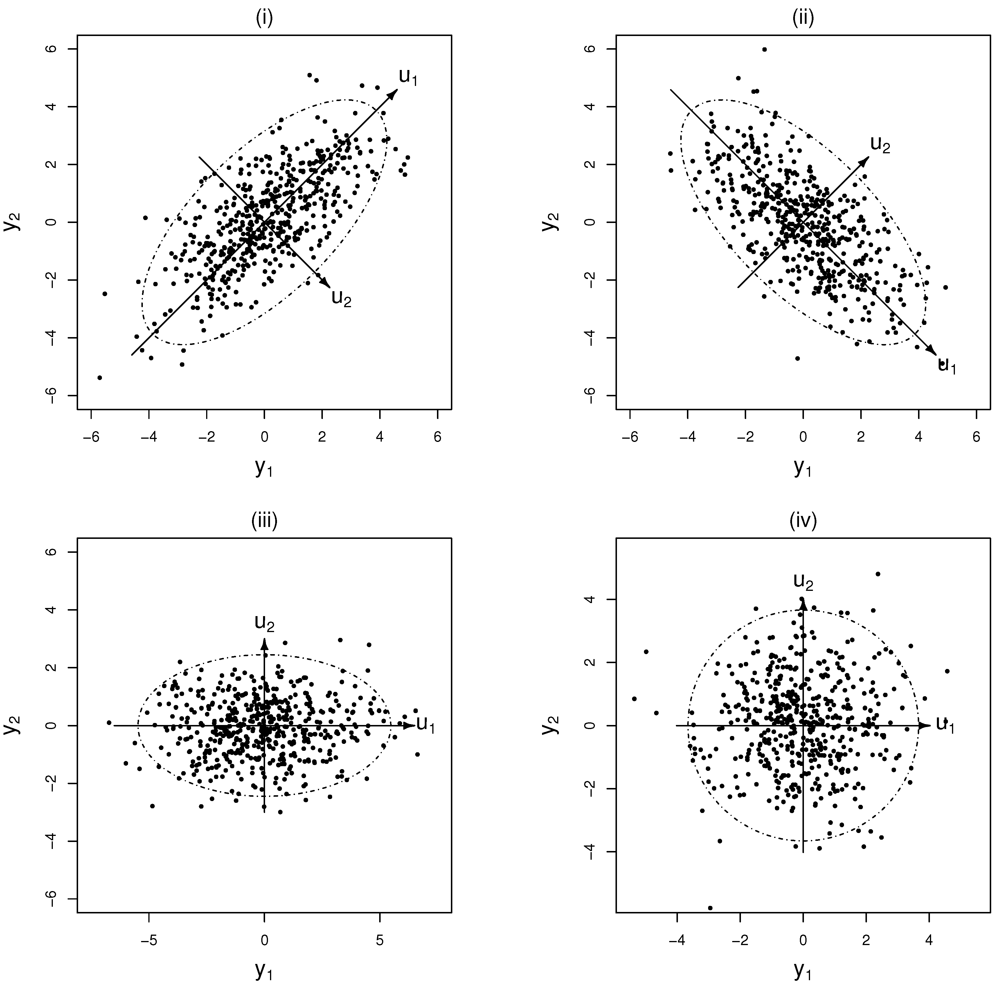The eigenvalues ${\lambda }_1\ge \cdots \ge {\lambda }_k\ge 0$ are nonnegative since $\mathsf{\Sigma }$ is positive semidefinite. For a simple illustration, let us consider Figure 1, the scatter plots of the normal random numbers with ellipses of 95% confidence interval, when the variance matrices are, respectively, $S_1,S_2$, $S_3$, and $S_4$:

$$S_1=\left(\begin{array}{cc}3& 2\\ 2& 3\end{array}\right),S_2=\left(\begin{array}{cc}3& -2\\ -2& 3\end{array}\right),S_3=\left(\begin{array}{cc}5& 0\\ 0& 1\end{array}\right),S_4=\left(\begin{array}{cc}\sqrt{5}& 0\\ 0& \sqrt{5}\end{array}\right).$$

(3)

The eigenvalues of $S_1,S_2$, and $S_3$ are the same, namely, ${\lambda }_1=5$ and ${\lambda }_2=1$, while for $S_4$, ${\lambda }_1={\lambda }_2=\sqrt{5}$. The eigenvalues ${\lambda }_1,{\lambda }_2$ represent the distances from the center to the surface of the ellipsoid, while the eigenvectors $u_1,u_2$ provide the directional information of the distribution. In other words, ${\lambda }_1$ and ${\lambda }_2$ tell us how the dataset is spread out along the principal components, which are the eigenvectors.

Generalized variance (GVAR) summarizes the distances in all directions

$$GVAR=\left|\mathsf{\Sigma }\right|=\prod _{i=1}^k{\lambda }_i,$$

thus giving us a scalar quantity in place of $k(k+1)/2$ distinct elements. It is not surprising that GVAR is computed only with the eigenvalues, disregarding the eigenvectors (which convey the information about positive/negative correlation, as in Figure 1), since it measures the size of overall pure variability of the multivariate system, not the directions of its movements.

It is, however, desirable to complement $\left|\mathsf{\Sigma }\right|$ with additional information about the system variation. As shown above, the eigenvalues decompose the overall variability in k directions. Reporting the individual values ${\lambda }_1,{\lambda }_2,\cdots ,{\lambda }_k$ along with GVAR will therefore be useful for obtaining a better and broader picture of variability.

2.2. Statistical Properties of the Generalized Variance

The GVAR has an undesirable property that it depends on the units of measurement. By partitioning the $k\times k$ dimensional matrix $\mathsf{\Sigma }$ (now denoted as ${\mathsf{\Sigma }}_k$), we can write:

$$\begin{array}{cc}\hfill |{\mathsf{\Sigma }}_k|& =\left|\begin{array}{cc}{\mathsf{\Sigma }}_{k-1}& {\sigma }_{1,\cdots ,k-1;k}\\ {\sigma }_{k;1,\cdots ,k-1}^{\prime }& {\sigma }_k^2\end{array}\right|\hfill \\ \hfill & =|{\mathsf{\Sigma }}_{k-1}|({\sigma }_k^2-{\sigma }_{k;1,\cdots ,k-1}^{\prime }{\mathsf{\Sigma }}_{k-1}^{-1}{\sigma }_{1,\cdots ,k-1;k}).\hfill \end{array}$$

Using the formula for the multiple correlation coefficient $R_{k;1\cdots k-1}$ (see Anderson (1984, p. 39) for details),

$$R_{k;1\cdots k-1}=\frac{\sqrt{{\sigma }_{k;1,\cdots ,k-1}^{\prime }{\mathsf{\Sigma }}_{k-1}^{-1}{\sigma }_{1,\cdots ,k-1;k}}}{{\sigma }_k},$$

the determinant $|{\mathsf{\Sigma }}_k|$ can now be expressed as:

$$|{\mathsf{\Sigma }}_k|=|{\mathsf{\Sigma }}_{k-1}|{\sigma }_k^2(1-R_{k;1\cdots k-1}^2).$$

(4)

Thus, we can make $|{\mathsf{\Sigma }}_k|$ greater (or smaller) than $|{\mathsf{\Sigma }}_{k-1}|$ by choosing the units of the kth variable $Y_k$ in such a way that $V\left(Y_k\right|Y_{1,\cdots ,k-1})={\sigma }_k^2(1-R_{k:1\cdots k-1}^2)$ is greater (or smaller) than one.

The generalized variance, however, is invariant under rotation. It does not change by the multiplication of the variance matrix with a rotational matrix L whose determinant is 1, since $\left|L\mathsf{\Sigma }\right|=\left|L\right|\left|\mathsf{\Sigma }\right|=\left|\mathsf{\Sigma }\right|$. The matrices $S_2,S_3$, and $S_4$ can be obtained from $S_1$ by premultiplying, respectively, with the rotational matrices $L_2,L_3$, and $L_4$:

$$L_2=\left(\begin{array}{cc}13/5& -12/5\\ -12/5& 13/5\end{array}\right),L_3=\left(\begin{array}{cc}3& -2\\ -2/5& 3/5\end{array}\right),L_4=\left(\begin{array}{cc}3/\sqrt{5}& -2/\sqrt{5}\\ -2/\sqrt{5}& 3/\sqrt{5}\end{array}\right).$$

Even though the four populations corresponding to $S_i(i=1,2,3,4)$ differ in their shape, the areas (i.e., the determinants) of the ellipses in Figure 1 covering 95% of the scattered points (assuming bivariate normality) are the same. This result is not surprising, given that GVAR measures the overall variance of the multivariate system, disregarding the distributional shape.

We now discuss an important result relating to the determinants of two variance matrices ${\mathsf{\Sigma }}_1$ and ${\mathsf{\Sigma }}_2$ (see Horn and Johnson (1985, p. 471)), which will further strengthen the importance of generalized variance as a measure of overall variability.

Proposition 1. 

Let ${\mathsf{\Sigma }}_1$ and ${\mathsf{\Sigma }}_2$ be the two variance matrices, of which ${\mathsf{\Sigma }}_2$ is nonsingular. Then, ${\mathsf{\Sigma }}_2\ge {\mathsf{\Sigma }}_1$ (i.e., ${\mathsf{\Sigma }}_2-{\mathsf{\Sigma }}_1$ is positive semidefinite) implies $|{\mathsf{\Sigma }}_2|\ge |{\mathsf{\Sigma }}_1|$.

Note that the reverse of this result may not be true, which can be easily seen by the following simple counter-example. Taking

$${\mathsf{\Sigma }}_1=\left(\begin{array}{cc}2& 1\\ 1& 2\end{array}\right)\mathrm{and}{\mathsf{\Sigma }}_2=\left(\begin{array}{cc}2& 0\\ 0& 2\end{array}\right),$$

we have $|{\mathsf{\Sigma }}_2|\ge |{\mathsf{\Sigma }}_1|$; however, ${\mathsf{\Sigma }}_2-{\mathsf{\Sigma }}_1$ is not positive semidefinite. Therefore, the positive semidefiniteness of ${\mathsf{\Sigma }}_2-{\mathsf{\Sigma }}_1$ is a sufficient (but not a necessary) condition for “more” variability. As a test for parameter stability, Rigobon (2003) proposed the determinant of the change in the variance matrix (DCVM) defined as:

$$DCVM=\frac{|{\widehat{\mathsf{\Sigma }}}_2-{\widehat{\mathsf{\Sigma }}}_1|}{\widehat{\sigma }},$$

(5)

where ${\widehat{\mathsf{\Sigma }}}_2$ and ${\widehat{\mathsf{\Sigma }}}_1$ are the estimated variance matrices of asset returns, respectively, for the periods 2 and 1, and $\widehat{\sigma }$ is the relevant standard error. Dungey et al. (2004) went one step further to claim that if the volatility increases during period 2, then $DCVM>0$. However, given our above discussion, volatility during period 2 can be larger even when $DCVM<0$. Proposition 1 clearly shows that a relevant quantity to consider should be $|{\widehat{\mathsf{\Sigma }}}_2|-|{\widehat{\mathsf{\Sigma }}}_1|$ scaled by an appropriate standard error.

2.3. Scatter Coefficient

Frisch (1929)’s scatter coefficient, denoted as $|R_k{|}^{1/2}$ for k variables, is a measure of the degree of “non-singularity” of the distribution. It will reach its maximum when any two vectors of observations ${(y_{i1},\cdots ,y_{in})}^{\prime }$ and ${(y_{j1},\cdots ,y_{jn})}^{\prime }$ ($i\ne j$) are orthogonal, or in other words, the variables $Y_i$ and $Y_j$ are independent for all $i,j=1,\cdots ,k$. On the other hand, it will be smaller when two or more of these vectors are oblique. Using (1) and by repeated application of Equation (4), we have:

$$|R_k{|}^{1/2}={(1-R_{k:1\cdots k-1}^2)}^{1/2}{(1-R_{k-1:1\cdots k-2}^2)}^{1/2}\cdots {(1-R_{2:1}^2)}^{1/2},$$

(6)

where the ith term $(i=1,2,\cdots ,k-1)$ on the right hand side represents the proportion of unexplained variation in a regression of $y_{k-i+1}$ on $y_{k-i},y_{k-i-1},\cdots ,y_1$. Relationship (6) prompted Frisch (1929, p. 55) to comment, “The coefficient of scatter for a set of variables is never greater than the coefficient of scatter for a subset contained in the set”.

As an opposite quantity of the scatter coefficient, the collective correlation (CCOR)

$$CCOR={\left(1-|R_k|\right)}^{1/2}$$

can be used as a measure of the strength of linear dependence. This measure is invariant to the shape of the scattered observations. For example, in Figure 1, diagrams (i) and (ii) have the same CCOR, 2/3, while for (iii) and (iv), it is obviously zero. This result is natural, considering that CCOR measures the strength, not the direction, of overall dependence.

2.4. Modifications of GVAR and CCOR

The practical problem of GVAR is that its numerical value grows too big with the dimension k. Secondly, the variability in distributions of different dimensions cannot be compared with GVAR. To resolve these problems, it is desirable to average the eigenvalues ${\lambda }_1,\cdots ,{\lambda }_k$, rather than simply multiplying them. Peña and Rodriguez (2003) proposed the geometric mean of eigenvalues as the effective variance (EVAR):

$$EVAR=|{\mathsf{\Sigma }}_k{|}^{1/k}=({\sigma }_1^2{\sigma }_2^2\cdots {\sigma }_k^2|R_k{\left|\right)}^{1/k}={\left(\prod _{i=1}^k{\lambda }_i\right)}^{1/k}.$$

(7)

It can also be interpreted as the average length of the side of a hypercube whose volume is equal to $|{\mathsf{\Sigma }}_k|$. We suggest the generalized standard deviation, GSD, and effective standard deviation, ESD:

$$GSD={GVAR}^{1/2},ESD={EVAR}^{1/2}.$$

(8)

Especially ESD is very helpful for understanding the overall variability since it has the same scale of the individual variables.

Similarly, to get around the problem that $CCOR=(1-|R_k{\left|\right)}^{1/2}$ always increases with the additional variable(s), Peña and Rodriguez (2003) proposed the following measure, which we will call an effective correlation (ECOR) coefficient:

$$ECOR=1-|R_k{|}^{1/k}=1-{\left(\prod _{i=1}^k{\gamma }_i\right)}^{1/k},$$

(9)

where ${\gamma }_i$s are the eigenvalues of the correlation matrix $R_k$.

3. An Empirical Application

Scalar summaries of all the variance–covariances and correlations in the multivariate system can be conveniently applied to many research areas in economics and finance. For example, these measures can be straightforwardly applied to the comovement phenomenon, often observed in the international financial markets and one of the most actively discussed topics in financial economics. Previous literature on the inter-market dependence employed numerous t-tests on the possible change of many pairwise correlations between markets. However, the measure summarizing all the correlations into a single number will be a convenient tool to provide a more definite answer to whether the market comovements increased or not.

As the last three decades have witnesses a series of financial crises all over the world, many economists and policy makers were interested in understanding if and how the negative shocks are transmitted across borders. They used a plethora of empirical methodologies to test for market comovements due to contagion: cross-market correlation coefficients, GARCH models, and direct estimation of specific transmission mechanisms. However, the most straightforward and most widely employed approach to test for market comovements is the use of cross-market correlation coefficients. Calvo and Reinhart (1996) found a rise in correlation between returns on equities and Brady bonds for Asian and Latin American emerging markets after the Mexican crisis. Bekaert et al. (2016) used equity return correlations among 58 countries to show a substantial increase in global comovements. Recently, Tilfani et al. (2020) studied temporal variation of detrended cross-correlation coefficients between stock markets of the Eurozone countries. The authors found high levels of comovements between Germany and the EU countries after the sovereign debt crisis, although the Brexit decision reduced those connections.

On the other hand, Forbes and Rigobon (2002) and Rigobon (2019) argued that the correlation test is biased due to the heteroskedasticity of asset returns. They showed that once the bias is adjusted, the evidence of contagion disappears in the Asian crisis of 1997, the Mexican crisis of 1994, and the US stock market crash of 1987. In response to Forbes and Rigobon’s argument, Bartram and Wang (2005) and Corsetti et al. (2005) claimed that the adjustment of Forbes and Rigobon (2002) produces serious biases favoring the null hypothesis of “no contagion”. The dynamic conditional correlation (DCC) GARCH model has been widely used to study time-varying cross-market correlations. Caporale et al. (2005) and Chiang et al. (2007) used the DCC-GARCH model to investigate contagion existence between the Asian stock markets. Gjika and Horvath (2013) argued for the stronger market comovements of Central Europe vis–à–vis the euro area, using the time-varying correlations estimated with the DCC-GARCH model.

Most of the testing methodologies mentioned above, focusing on the correlation among national stock markets, ended up with many pairwise comparisons of each of the individual correlation coefficients, presenting difficulties in reconciling conflicting movements. In most cases, the correlation coefficients between the markets even in the same region do not move in a unison pattern. Therefore, a definite conclusion would be difficult to attain. Scalar measures of volatility and correlation can help resolve this problem by directly measuring the changes in overall comovement among all the countries.

In this section, we will discuss the convenience and general applicability of the suggested measures using data on six Asian stock market returns. Specifically, we will demonstrate the changes of the regional volatility and the strength of the regional comovement, as opposed to the individual variances and correlations. GVAR and CCOR applied to the conditional variance (or correlation) matrix estimated from multivariate GARCH models produce indicators that are shown to be able to track the time variation in regional market volatilities and correlations.

3.1. Data and Descriptive Statistics

We used weekly (Wednesday close) stock return data, retrieved from Bloomberg, for six Asian markets: Japan (Nikkei225), Hong Kong (HangSeng), Singapore (STI), Korea (KOSPI), Thailand (SET), and Indonesia (JSX). The return series were calculated as 100.0 times log price differences in the local currency. The sample ran from 16 January 1985 to 29 March 2017, yielding 1531 observations. If any Wednesday observation was missing, Thursday’s index (Tuesday’s index if Thursday is still missing) was used. If the market was closed from Tuesday to Thursday, then the observation for that week was recorded as missing.

Table 1. Descriptive statistics of weekly returns on Asian stock indices. The table reports descriptive statistics for six Asian stock markets, Japan (Nikkei 225), Hong Kong (HangSeng), Singapore (STI), Korea (KOSPI), Thailand (SET), and Indonesia (JSX). We used weekly (Wednesday close) returns from 16 January 1985 to 29 March 2017, yielding 1531 observations. The pre-crisis period and post-crisis period are 16 January 1985 to 24 December 1997 and 14 January 1998 to 29 March 2017, respectively, which gives 613 and 918 observations, respectively.

	Japan	Hong Kong	Singapore	Korea	Thailand	Indonesia
	Full Sample Period
mean	0.036	0.193	0.093	0.127	0.114	0.190
standard deviation	2.972	3.305	2.866	3.614	3.570	3.273
skewness	−0.213	−0.519	−0.092	−0.126	−0.175	−0.076
kurtosis	4.772	5.787	6.258	6.681	5.830	8.207
JB test	213.41 **	567.19 **	682.83 **	872.28 **	521.43 **	1738.36 **
$Q\left(5\right)$	1.49	3.37	15.70 **	24.27 **	24.53 **	51.13 **
$Q^2\left(5\right)$	137.97 **	228.65 **	181.13 **	394.65 **	199.25 **	322.97 **
	Pre-Crisis
mean	0.054	0.355	0.143	0.115	0.134	0.146
standard deviation	2.774	3.273	2.901	3.403	3.707	2.912
skewness	−0.375	−1.047	−0.455	−0.274	−0.519	0.426
kurtosis	5.143	7.150	5.689	7.468	5.165	8.983
JB test	133.50 **	557.27 **	208.50 **	523.28 **	149.24 **	941.81 **
$Q\left(5\right)$	10.83	8.68	3.07	9.45	18.03 **	72.60 **
$Q^2\left(5\right)$	143.18 **	48.96 **	69.45 **	122.03 **	95.20 **	123.60 **
	Post-Crisis
mean	0.025	0.085	0.060	0.135	0.101	0.219
standard deviation	3.098	3.324	2.845	3.751	3.477	3.495
skewness	−0.132	−0.181	0.164	−0.052	0.102	−0.276
kurtosis	4.532	5.038	6.685	6.227	6.357	7.657
JB test	93.62 **	165.58 **	527.53 **	402.10 **	436.15 **	847.27 **
$Q\left(5\right)$	3.50	6.63	14.50 *	18.20 **	13.36 *	19.62 **
$Q^2\left(5\right)$	39.50 **	241.15 **	119.93 **	212.87 **	119.63 **	189.86 **

* and ** indicate statistical significance at the 5% and 1% levels, respectively.

reports the summary statistics for each country. Asian markets exhibited a positive average return during the sample period. As expected, the mature markets such as Japan, Hong Kong, and Singapore had the smaller standard deviation. Significant non-normality was confirmed by the Jacque–Bera (JB) test statistics. The Ljung–Box Q-statistics with five lags indicated a significant serial dependence of returns for Singapore, Korea, Thailand, and Indonesia and a lack of it for Japan and Hong Kong. The squared returns, as evident from the values of $Q^2\left(5\right)$, have strong serial correlation for all countries, indicating the presence of nonlinear dependence and conditional heteroskedasticity.

In the post-crisis period, the stock markets of Korea, Thailand, and Indonesia performed much better in terms of average return than the mature markets. Inference on the distributional properties such as the non-normality and the heteroskedasticity did not change over the two subperiods. One particularly distinctive feature between subperiods is that the individual volatility of most markets increased after the crisis, except Thailand, which exhibited slightly lower volatility.

3.2. Market Comovements and Volatility

Prior to studying the dynamic aspects of the regional volatility and dependence, we studied the changes in overall volatility and comovement of the Asian markets between the periods 1985–1997 and 1998–2017.

Table 2. Volatility and correlation in the periods 1985–1997 and 1998–2017.

Periods	1985–1997		1998–2011
# of Obs	613		631
	Volatility	Correlation	Volatility	Correlation
GVAR	$4.309\times {10}^5$	-	$1.002\times {10}^5$	-
GSD	656.43	-	316.57	-
EVAR	8.69	-	6.82	-
ESD	2.95	-	2.61	-
CCOR	-	0.73	-	0.97
ECOR	-	0.12	-	0.38

presents the changes in overall measures of regional volatility and comovement during the pre-crisis and post-crisis periods. All the volatility measures indicate a substantial decrease in the overall volatility in the post-crisis period compared to the pre-crisis period. The decrease of the regional volatility in the post-crisis period clearly contradicts the fact, found in Table 1, that the standard deviation of most market returns actually increased after the crisis.

This seemingly inconsistent result is not surprising, considering that the generalized variance is essentially the volume of the ellipsoid covering the market return data. Before the crisis, the six market returns are less correlated and hence more scattered around the six-dimensional space, so that the ellipsoid they form is more round in shape. Contrastingly, the market data in the post-crisis period constitute the more elongated ellipsoid, reflecting a closer interdependence among the markets. Therefore, although each stock market became more volatile in the post-crisis period, their strongly concentrated movements after the crisis elongated the ellipsoid covering the data and shrank the volume of the ellipsoid, leading to a decrease in the regional volatility.

A significant increase of the overall correlation in the recent decade was confirmed by both the collective correlation (CCOR), ${(1-|R\left|\right)}^{1/2}$, and effective correlation (ECOR). The effective correlation demonstrated a more noticeable increase from 0.12 to 0.38 after the crisis.

We now turn to the issue of the link between the volatility and correlation across national markets, which is another important issue in international finance literature. Correlations between equity markets are often claimed to increase during the periods of market turbulences. To examine whether the regional comovement was stronger in the volatile period than in the tranquil period, we need to split the sample into the volatile and stable periods. Each week of the market returns were assigned to the volatile and tranquil periods by the regional volatility on that week.

For this dating procedure, the weekly volatility of each market was first estimated with AR(1) with GARCH(1,1) model: ’Each weeks of’:

$$y_{it}={\mu }_i+{\theta }_i{y}_{it-1}+{ϵ}_{it},$$

(10)

where:

$$\begin{array}{cc}\hfill & {ϵ}_{it}|I_{t-1}\sim N(0,h_{it})\hfill \end{array}$$

(11)

$$\begin{array}{cc}\hfill & h_{it}={\omega }_i+{\alpha }_i{ϵ}_{i,t-1}^2+{\beta }_i{h}_{i,t-1},\hfill \end{array}$$

(12)

for $i=1,2,\cdots ,6$ countries, with $I_{t-1}$ denoting the past information set. The estimation results are reported in

Table 3. Estimation results.

	$\widehat{\mathit{\mu }}$	$\widehat{\mathit{\theta }}$	$\widehat{{\mathit{\omega }}_{\mathit{i}}}$	$\widehat{{\mathit{\alpha }}_{\mathit{i}}}$	$\widehat{{\mathit{\beta }}_{\mathit{i}}}$
Japan	0.161	−0.007	0.672	0.149	0.783
	(2.22)	(−0.24)	(1.95)	(4.43)	(15.81)
Hong Kong	0.261	0.024	0.495	0.135	0.821
	(3.50)	(0.88)	(2.69)	(4.53)	(22.08)
Singapore	0.135	0.054	0.134	0.096	0.892
	(2.10)	(1.82)	(1.55)	(3.61)	(26.91)
Korea	0.192	0.008	0.147	0.142	0.857
	(2.89)	(0.29)	(1.77)	(4.53)	(28.99)
Thailand	0.181	0.064	0.242	0.123	0.864
	(2.16)	(2.31)	(1.95)	(3.87)	(23.93)
Indonesia	0.196	0.132	0.058	0.104	0.895
	(2.84)	(4.20)	(1.24)	(6.28)	(50.41)

The t-values are given in parentheses.

.

To measure the regional volatility for dating volatile and tranquil periods, we used the geometric average of the product of individual conditional variances to define the total variance, ${TVAR}_t$:

$${TVAR}_t={(h_{1t}\cdots h_{6t})}^{1/6},$$

(13)

and the total standard deviation, ${TSD}_t={TVAR}_t^{1/2}$. The GVAR is not a proper summary of the regional volatility for this study, because it contains the information about the market comovement. The weeks in which the total standard deviation ${TSD}_t$ was in excess of a particular threshold were dated as the volatile periods. The remaining periods were assigned to the tranquil periods. We selected two threshold values: 3.0 and 3.5.

Table 4. Changes in correlation between volatile and tranquil periods.

Threshold Values for TSD	3.0		3.5
Periods	Tranquil	Volatile	Tranquil	Volatile
Number of Obs	967	564	1208	323
CCOR	0.845	0.950	0.853	0.968
ECOR	0.189	0.322	0.195	0.369

reports the correlation measures in the tranquil and volatile periods. The collective correlation measures CCOR and ECOR clearly indicate that the market comovement became stronger in the volatile periods. The difference of collective correlations between volatile and tranquil periods became wider as the threshold (for classifying volatile observations) became higher from 3.0 to 3.5. This demonstrates that the scalar measures are very useful for providing definite evidence that the market comovement becomes stronger with the severity of the regional volatility.

3.3. Instantaneous Measures of the Regional Volatility and Correlation

We now demonstrate that the generalized variance and collective correlation, when combined with the multivariate GARCH model, can provide the time variation in overall volatilities and correlations of multiple markets. Among many recent multivariate GARCH models, we used the dynamic conditional correlation (DCC) MGARCH of Engle (2002) and Tse and Tsui (2002).

In the DCC-MGARCH model of Engle (2002), the conditional variance matrix $H_t$ of the error term, ${ϵ}_t={({ϵ}_{1t},{ϵ}_{2t},\cdots ,{ϵ}_{kt})}^{\prime }$ in the mean Equation (10), is decomposed as follows:

$$H_t=D_t{R}_t{D}_t,$$

(14)

where the matrix $D_t=diag(\sqrt{h_{1t}}\cdots \sqrt{h_{kt}})$ is constructed with the conditional variance $h_{it}$ of the univariate GARCH as in Equation (12) and the dynamic conditional correlation matrix $R_t$ is written as:

$$R_t=diag(1/\sqrt{q_{11,t}}\cdots 1/\sqrt{q_{kk,t}})Q_{t}diag(1/\sqrt{q_{11,t}}\cdots 1/\sqrt{q_{kk,t}}).$$

(15)

The $k\times k$ symmetric positive definite matrix $Q_t$ is given by

$$Q_t=(1-a-b)\overline{Q}+a{u}_{t-1}{u}_{t-1}^{\prime }+b{Q}_{t-1},$$

(16)

where $u_{it}={ϵ}_{it}/\sqrt{h_{i,t}}$ denotes the standardized residual, and the matrix $\overline{Q}$ is the unconditional covariance matrix of $u_t$.

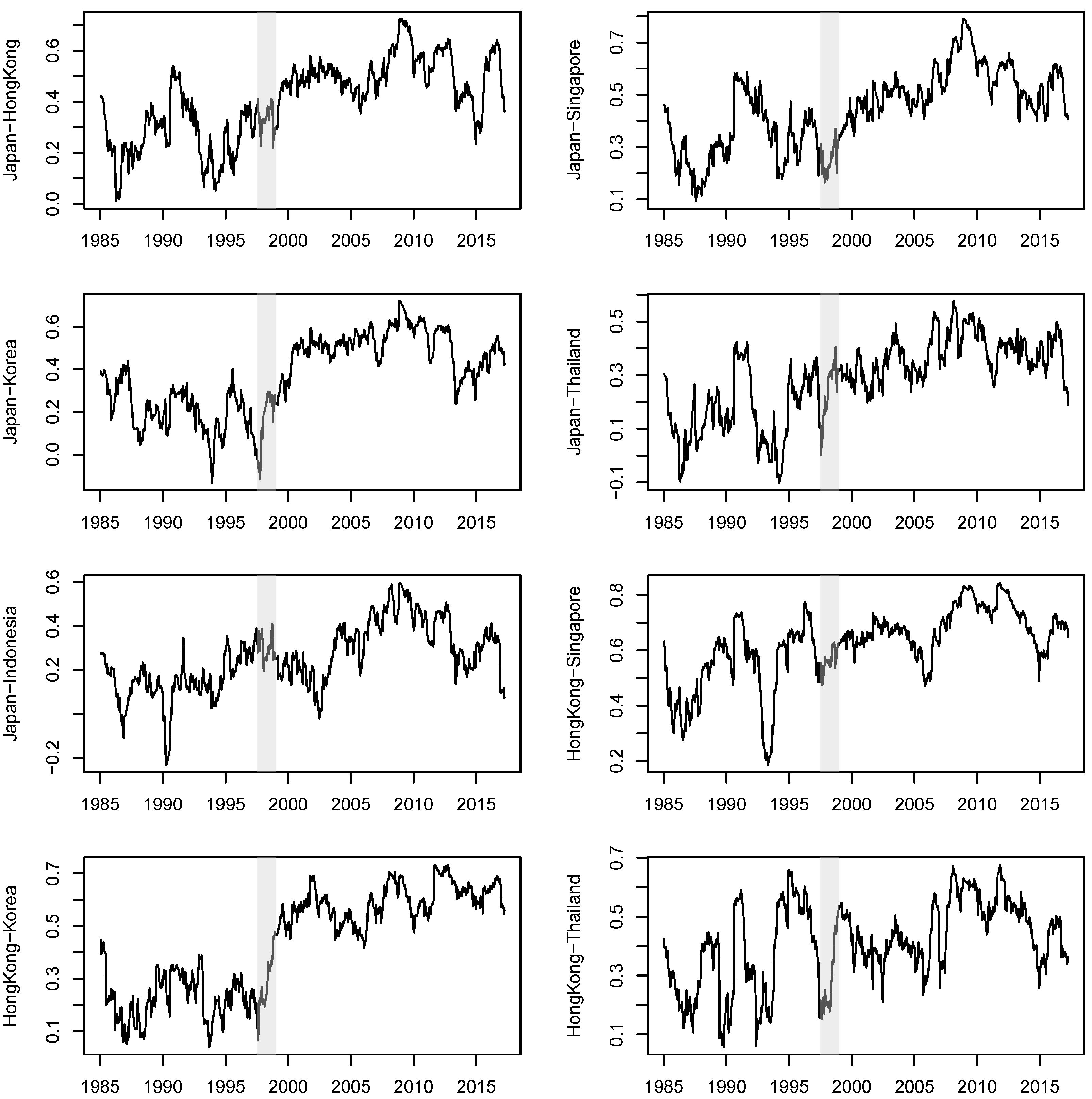
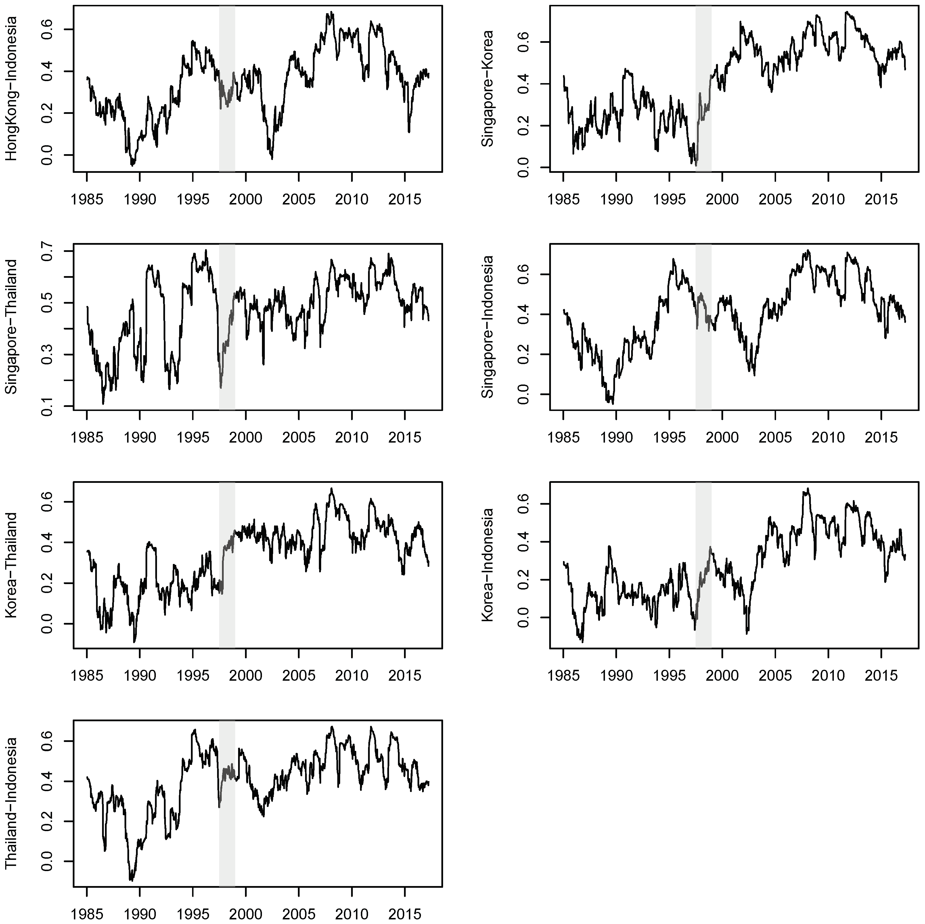
The GARCH coefficients of $Q_t$ in (16) were estimated to be $\widehat{a}=0.023\left(5.94\right),$$\widehat{b}=0.968\left(138.58\right)$, where the figures in the parentheses are the t-values. This provides strong evidence of time-varying conditional correlations. The pairwise conditional correlations between market returns are plotted in Figure 2. The stronger comovements in the post-crisis period can be visually confirmed in most pairs of countries, but it is not obvious in a few pairs such as for Hong Kong–Thailand and Singapore–Thailand. Therefore, it is not straightforward to draw any definite conclusion by looking at the movements of so many pairwise correlations.

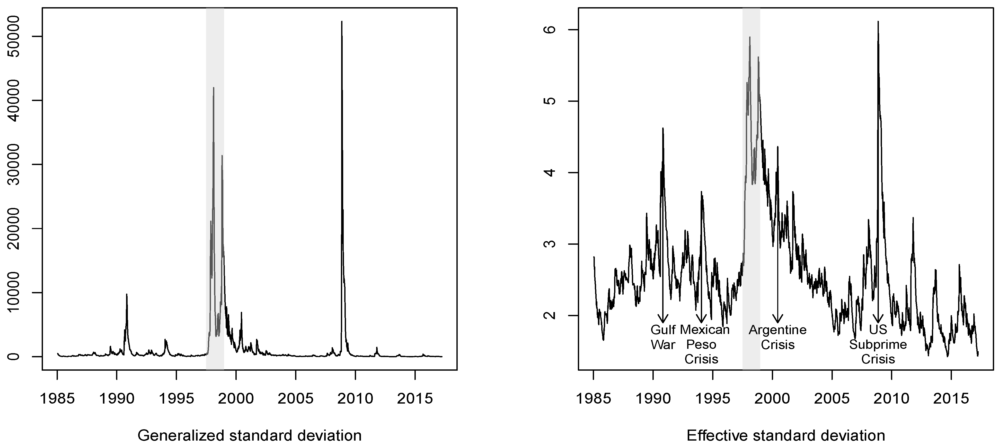
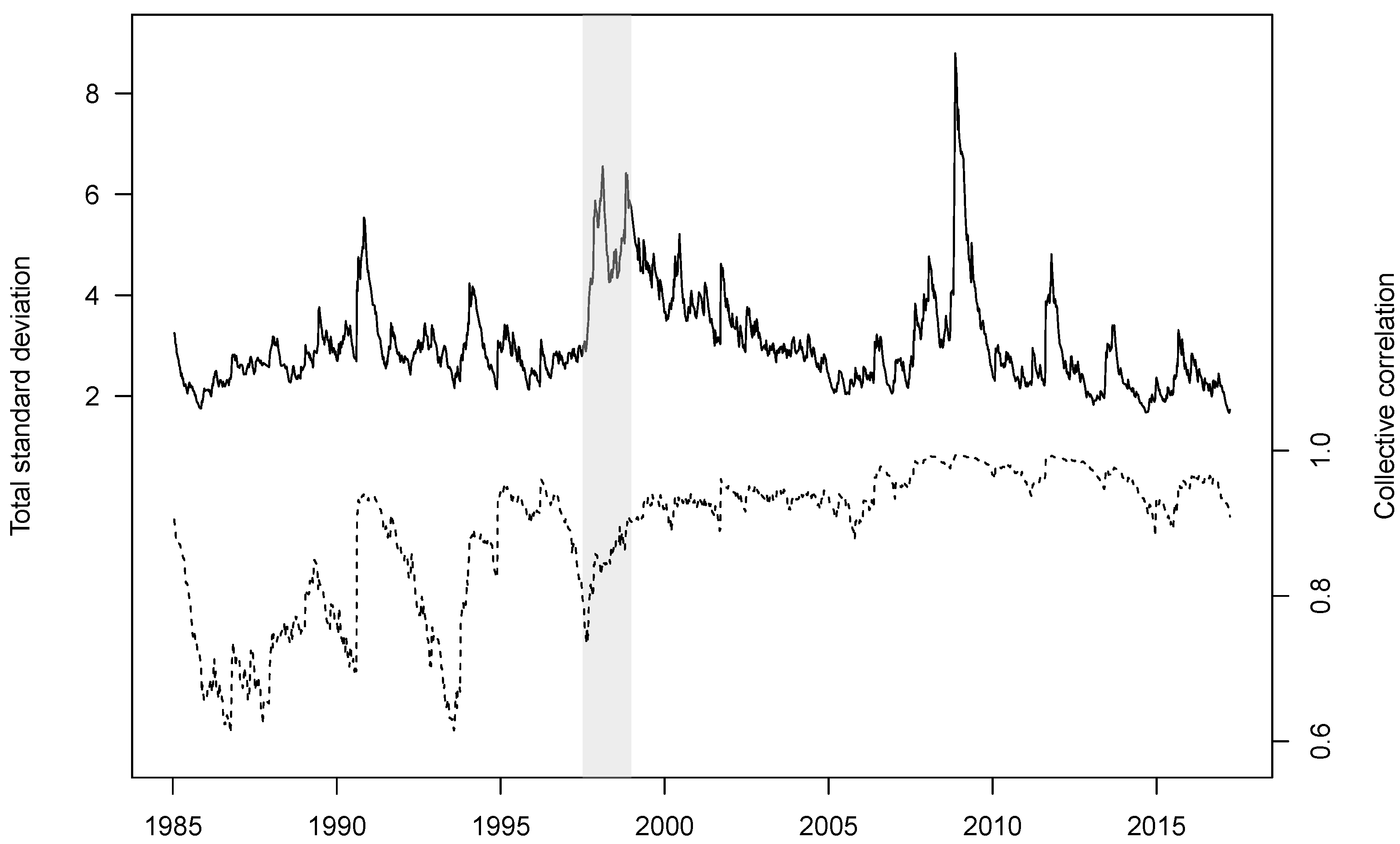
In Figure 3, the plot of ${GSD}_t$ (the standard deviation version of ${GVAR}_t$) distinctly shows the events of extreme volatility, such as the Asian crisis in 1997 and the recent subprime crisis in US (2008–2010). The medium-scale volatile events are overshadowed by the extremely high volatility peak of both crises. By contrast, the geometric average version ${ESD}_t$ has a much smaller range (from 2.0 to 6.0), and reveals other episodes of turbulence more clearly. For example, even the damaging impacts from the Mexican Peso crisis in 1994 and the Argentine financial crisis beginning in 2000 can be detected from the two smaller sharp kinks in ${ESD}_t$, while these were somewhat obscured in the graph of ${GSD}_t$.

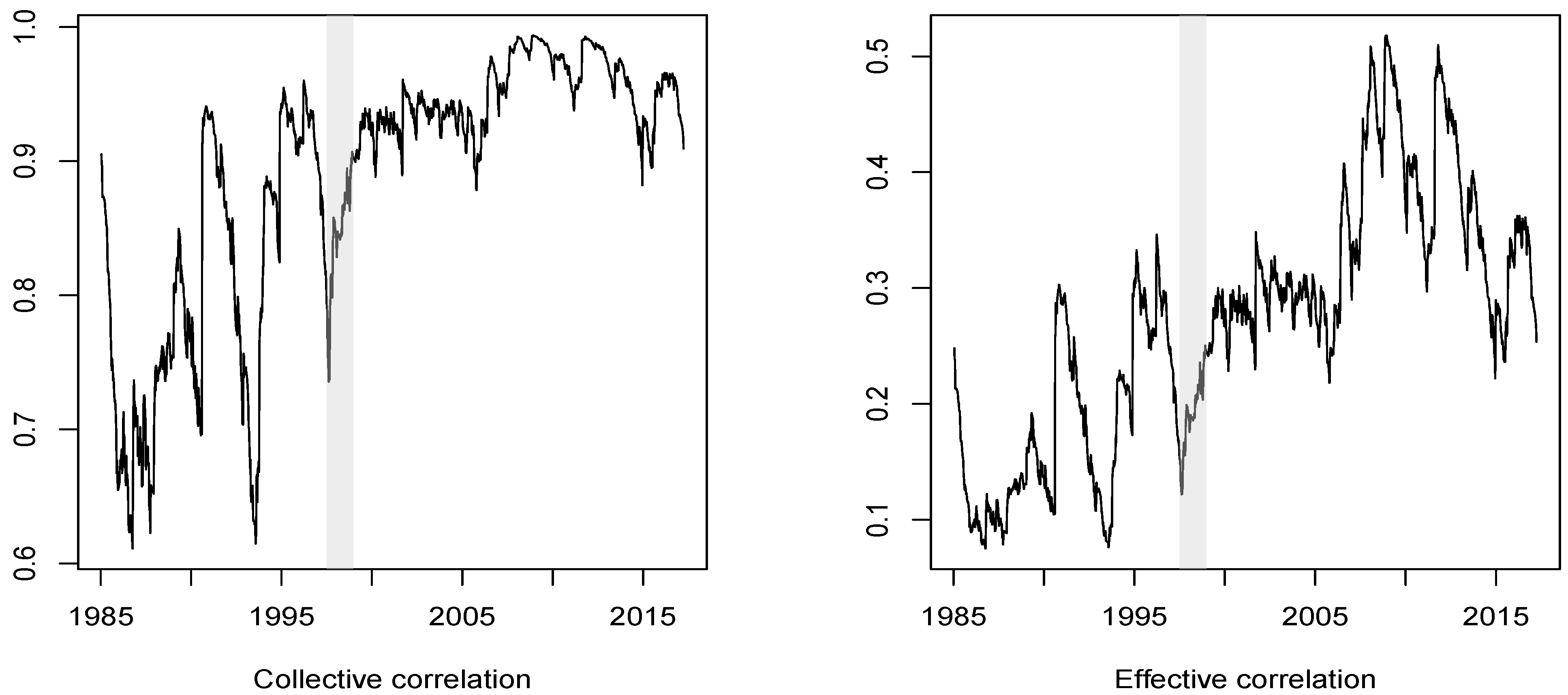
The plot of collective correlation (${CCOR}_t$) in Figure 4 confirms the upward drift of the regional correlation over the entire sample period while displaying substantial up and down irregularities. In the second plot of Figure 4, the pattern of increasing regional correlation is more pronounced when displayed using the geometric average version, i.e., the effective correlation (${ECOR}_t$).

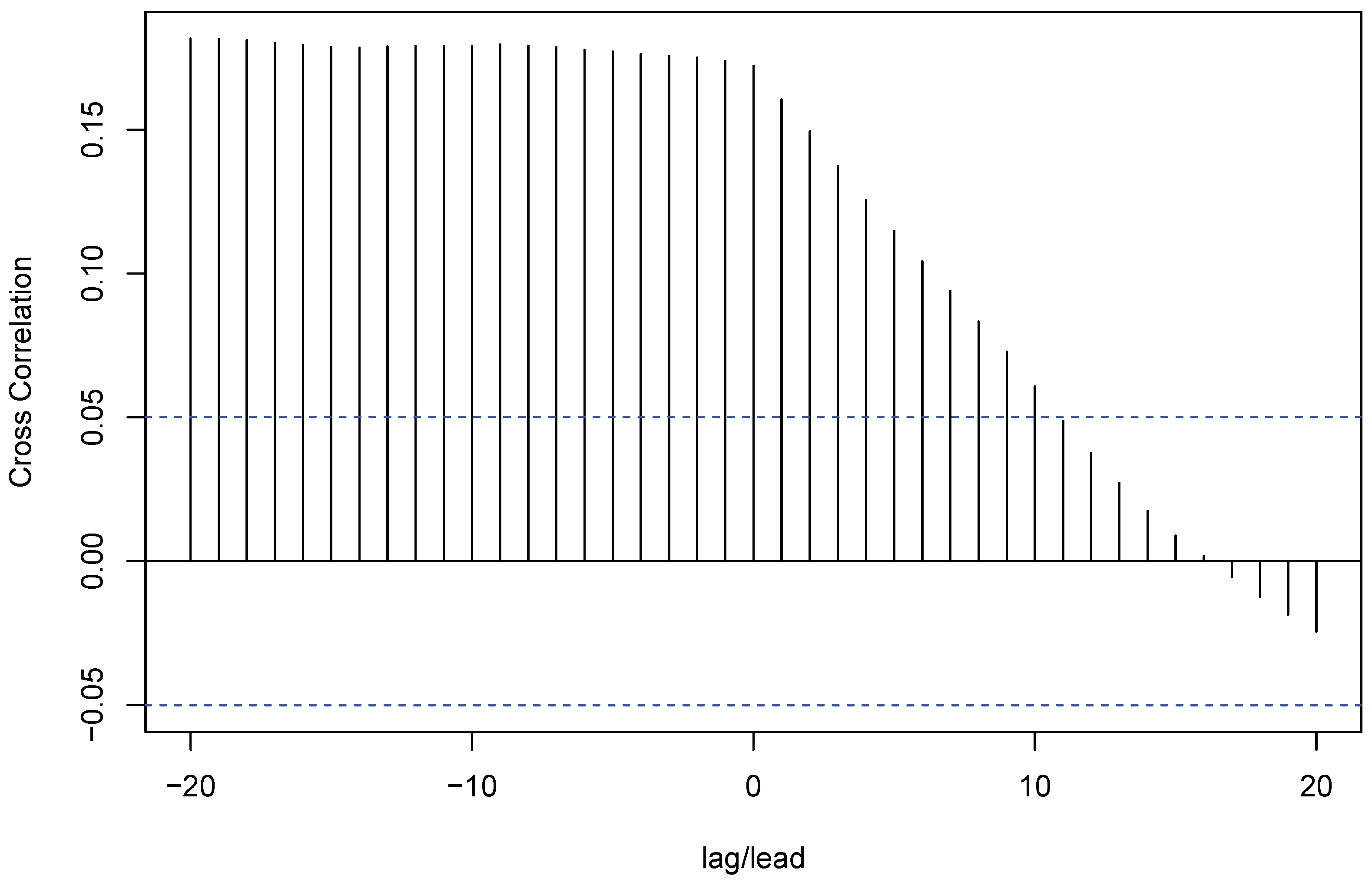
Let us now study the relationship between market comovement and volatility. Figure 5 suggests graphical evidence that market comovement measured by ${CCOR}_t$ becomes stronger during the periods of higher ${TSD}_t$. In addition, for a more rigorous test of contagion, defined by Forbes and Rigobon (2002) as “a significant increase in cross-market linkages after a shock to one country (or group of countries)”, we calculated the lead-lag relationship between the volatility and market comovement. In Figure 6, we plot the cross serial-correlations between the volatility ${TSD}_{t+j}$ and regional comovement ${ECOR}_t$ at lag/lead $j=-20,-18,\cdots ,+20$. We notice a strong positive correlation between the lagged volatility shock ${TSD}_t$ and the regional dependence ${ECOR}_t$. When lead values of ${TSD}_{t+j}$ are considered, the serial correlations becomes much weaker. This provides strong evidence for the existence of contagion.

4. Conclusions

This paper is a first attempt to apply the concepts of generalized variance and collective correlation to financial data. These two statistics, respectively, provide simple measures of the overall variability and the dependence of a multivariate system by converting $k(k+1)/2$ numbers in the variance and correlation matrices to scalars. Both measures have intuitive geometric interpretations, and have much potential for further usefulness through their close relationships with principal component analysis. Some modifications on the generalized variance and collective correlation are recommended. For the generalized variance, we showed that by taking a geometric average it is possible to compare the results for two (or more) populations of different dimensions. Thus, using our technique, one can compare the overall market volatilities of two regions such as Asia and Europe of which the number of financial markets are different.

The scalar measures introduced in this paper performed the intended roles successfully in an empirical application to the six Asian market returns and, in addition, were shown to be able to reveal empirical facts which could not be uncovered by the traditional methods. Particularly, we showed that both the contagion and interdependence between the national equity markets could be confirmed more clearly. Moreover, the generality of the statistics proposed in this paper can be applied to any field in economics and finance, where the scalar measures of overall variability and dependence are needed.

There is a limitation of the use of scalar measures of overall volatilities presented in this paper. It would be nice to have the standard errors of our measures so that proper statistical inference can be conducted. It would not be an easy task to develop a rigorous methodology for inference on generalized variance and scatter coefficients in a multivariate GARCH setup. We would like to tackle this difficult problem in our follow-up research.