Abstract
This paper illustrates an innovative approach to financial modeling of engineering decision-making
and industrial projects. The approach is a minimal one, grounded as it is on three notions, two
laws, and one matrix that combines them, called Split-Screen Matrix (SSM). This split-screen approach
consists in linking the accounting and financial input data and systematizes them into the SSM, whose
columns report the pro forma book values of capital (balance sheets), the corresponding income
components (income statements), and the associated cash flows (cash-flow statements) while the rows
show the project’s dynamical evolution. The SSMs are then linked via a continuous split-screen strip.
To appraise the project, we use a pair of SSMs, namely, the project matrix and the benchmark Matrix
(with the related strips), the latter containing the alternative amount invested and the associated
foregone profit of a financial portfolio replicating the project’s cash flows. Using differences between
the corresponding elements of the two strips, the economic profitability of the project can be easily
measured, in both absolute terms (e.g., net present value, market value added, residual income) and
relative terms (e.g., average return on assets, cash-flow return on capital). The accounting-and-finance
engineering system (AFES) obtained with the split-screen approach is particularly helpful when using
spreadsheet modeling because it does not require (knowledge and) use of financial spreadsheet
functions. The application of this approach on spreadsheet modeling is essentially based on the
continuous split-screen strip, here described, and is illustrated in a following paper (Baschieri and
Magni 2023, “The Split-Screen Approach for Project Apraisal (Part II: Spreadsheet Modeling)”).
1. Introduction
Knowledge of accounting and financial magnitudes and its reciprocal relationships is important for appraising projects and firms. Analysts willing to evaluate projects or firms must reach a thorough understanding of both accounting notions and financial notions in order to build a rigorous and transparent modeling environment starting from the input data. On one hand, accounting notions are essential because a project’s or firm’s cash flows are estimated on the basis of pro forma financial statements (balance sheets, income statements, cash-flow statements), which are in turn drawn from the input parameters, which are estimation variables (e.g., prices and quantities of supplies and products, fixed costs, variable costs, labor costs, depreciation of fixed assets, taxes, etc.) and decision variables (credit terms, inventory policies, borrowing policy, payout policy, etc.); on the other hand, financial notions and principles are essential because the project’s value and/or the project’s financial efficiency are required to determine the cost of capital, COC (and the related notion of minimum attractive rate of return, MARR), which represents the expected rate of return of a financial asset traded in the security market comparable in risk to the project (Ross et al. 2011; Berk and DeMarzo 2014), and to make decisions: the analyst needs decision criteria capable of appraising a project and make an economically rational decision about whether the firm should undertake the project or not or about selection among several alternative investments.
For this reason, engineering economy textbooks and corporate finance textbooks devote adequate space to the illustration and explanation of accounting and financial magnitudes and their relationships (e.g., Damodaran 1999, 2006; Hartman 2007; Welch 2009, Newnan et al. 2009; Park 2013; Ross et al. 2013; Ehrhardt and Brigham 2016; Berk and DeMarzo 2014; Brealey et al. 2019).
An appropriate accounting-and-financial model describes a capital investment from the initial problem formulation up to the complete accounting-and-financial picture and then uses this picture to give rise to logically consistent evaluation and decision criteria. Mathematically, it may be viewed as a functional relation mapping a set of input parameters onto the model outputs (e.g., net present value, rate of return, profitability index, payback period, etc.) which may be used for solving different kinds of decision problems (e.g., accept/reject decisions, ranking of alternatives, allocations of resources to different projects or business units, etc.). (See Figure 1).
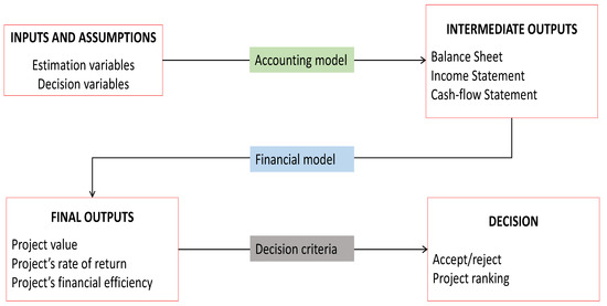
Figure 1.
Model structure for a capital asset investment.
The functional relation between input data and the model output(s) entails an intricate network of intermediate variables, such as several types of incomes (e.g., EBITDA, EBIT, gross profit, gross margin, earnings before taxes, net income), several types of capital (e.g., net fixed assets, operating working capital, debt capital, equity capital, liquid assets), and several types of cash flows (cash flow from assets, cash flow from operations, cash flow to equity, cash flow to debt). The model is a logical machine which activates a labyrinth of relations among the various incomes, cash flows and capital amounts and, therefore, among the financial statements (balance sheets, the income statements, and the cash-flow statements), and associates such magnitudes to financial, market-driven magnitudes such as the risk-adjusted COCs, representing the expected return on a replicating portfolio equivalent in risk to the project.
The model is made more complex by the fact that, in the set of inputs, estimation variables (e.g., prices and quantities) intertwine with decision variables under the managers’ control (e.g, the financing policy),1 a distinction which is usually neglected in the models currently available in engineering economics and operations research (and is totally neglected in practice by modelers).
In this paper, we illustrate an innovative accounting-and-finance modeling system, developed in Magni (2020) and named accounting-and-finance engineering system (AFES), which accomplishes the entire modeling process from the input data to the final outputs and the decision. We show how its use may favor financial modeling while boosting the rigour and the internal consistency of the financial model and reconciling seemingly conflicting measures of worth. Specifically, the AFES
- systematizes, in a transparent way, the links among the technical, accounting, and financial input data
- uses pro forma dynamical financial statements to carve out the project’s relevant magnitudes and, in particular, the four relevant areas of a project (operating, non-operating, debt, and equity)
- matches the three (pro forma) financial statements one against the other in the same visual representation and same working structure, called the Split-Screen Matrix (SSM), which enjoys invariance properties whereby effective accounting and financial information may be drawn regarding the project/firm with simple shifts and swaps of rows and columns
- derives a benchmark SSM describing the opportunity cost for each area of the project
- develops a split-screen strip for the project and a split-screen strip for the benchmark. Matching the former with the latter, it provides a class of consistent (absolute and relative) economically rational evaluation and decision criteria
- supplies several consistency checks to minimize the modeling errors
- translates the theoretical framework into unambiguous, logically consistent, and transparent spreadsheet modeling.
The approach presented is a frugal one, in that it uses three ingredients interconnected by two principles incorporated into one matrix. As such, this approach minimizes the cognitive effort for the modeler to learn it and use it.
The three ingredients represent the three ways a monetary amount can be conceptualized in economics: a capital amount, an income amount, or a cash flow amount. Any economic entity (be it a project, a firm, a loan, etc.) can be described in terms of such notions, and the link among them is based on the idea that the economic entity is a mechanical system, characterized by an amount of capital which is subject to forces exerted by agents (customers, suppliers, employees, debtholders, equityholders, government) who determine a static equilibrium, whereby the forces of investments and the forces of financings balance out. This equilibrium is determined by a law of conservation, which merely states that there is balance in economic activity. Specifically, capital invested is equal to capital raised; income generated is equal to income accrued; cash flow generated by an economic activity is equal to cash flow distributed to the capital providers; and rate of return generated from capital is equal to rate of return accrued to the capital providers. The economic system is equipped with a dynamics, and its law of motion merely states the capital position in one period is equal to the capital position from the previous period plus income (positive or negative) generated minus any cash flow paid out (or plus any cash flow contributed by the capital providers). As such, it resembles the dynamics of a saving account’s balance: the balance of the account increases (decreases) by a positive (negative) interest and decreases (increases) by a cash withdrawal (deposit).
Equipped with the three basic notions (capital, income, and cash flow) and the two laws (law of motion and law of conservation), we build what we call Split-Screen Matrix (henceforth, SSM), which portrays the static and dynamic dimension of investments and financings. Specifically, the rows of the SSM captures the dynamic dimension of the economic entity, while the columns of the same matric captures the static dimension.
The SSM is partitioned into four equipollent frames (screens) and enjoys important invariance properties, which turns the matrix into a shapeshifting logical machine equipped with a system of working rules, which we call split-screen technique. This technique enables manipulating accounting and financial magnitudes by performing simple operations (shifting or swapping rows/columns) in such a way that the balance sheet (BS), the income statement (IS), the cash-flow statement (CFS) are integrated and linked into a single visual representation. This format makes it easy to conceptualize complex relationships among accounting and financial magnitudes under four different-but-logically-equivalent perspectives, and accomplish a detailed analysis of the project’s economic efficiency and attractiveness. As for the latter issue, we stipulate and show that efficiency of a project and value creation is naturally modeled in terms of difference between the project Matrix and the associated benchmark Matrix, which describes the dynamics and statics of a replicating portfolio equivalent in risk to the project under consideration (its expected rate of return acting as the minimum attractive rate of return, MARR). The AFES favors the understanding and the treatment of accounting and financial relations and rationalizes the appraising process and the decision-making process while at the same minimizing the modeling errors.
This approach is particularly suited for spreadsheet modeling and its applications in digital environments are straightforward due to simple working rules that may be automatized easily. This paper represents the first part of a work that is completed by a second paper (Baschieri and Magni 2023), which will be entirely devoted to showing how to apply the theoretical framework illustrated in this part to spreadsheet modeling for real-world project appraisal.
Overall, compared with traditional financial modeling, we can summarize the major benefits of the AFES as follows:
- the underlying theory is frugal, for the whole model is grounded on two “laws” alone, which govern the whole network of accounting and financial relationships
- the continuous split-screen strip simplifies the spreadsheet modeling, enabling the modeler to use only two functions: INDEX and MATCH
- the AFES provides the tools for spotting internal inconsistencies, thereby ensuring correctness and precision
- the matrix layout guarantees transparency and optimal reading and interpretation, since,
- -
- horizontally, it associates the capital, income, and cash flow component of each area of business, and
- -
- vertically, it shows the financial statements as equilibria of capitals, incomes, and cash flows
- multiple measures of economic profitability are provided, all of which reciprocally consistent (and every one consistent with the NPV)
- the modeler does not need to be trained in accounting and finance to apply the AFES.
Pairing this paper with Baschieri and Magni (2023), where a detailed spreadsheet guide is presented, the easiness, effectiveness, and transparency of the AFES will be straightforward.
The remainder of the paper is structured as follows. Section 2 introduces the three basic notions and describes the law of motion (dynamics) and the law of conservation (statics). Section 3 makes use of these laws to build the SSM, showing the relations among the various areas of a project or firm (operating assets, liquid assets, debt, equity). Section 4 describes the split-screen technique. Section 5 shows the network of relations among the BS, the IS, and CFS and how to cope with them; it also shows how to reconcile the SSM with the standard financial statements. Section 6 shows how to pass from a classification of costs by nature to a representation of costs by function and the two framings of the project Matrix. Section 7 shows how to identify the gross profit, the EBITDA, the EBIT, and the Net Income on the SSM. Section 8 uses the SSM to introduce the notions of net operating working capital, net financial position, and operating cash flow. Section 11 introduces the notion of value and the benchmark Matrix, and shows how to calculate the Weighted Average Cost of Capital. Section 10 illustrates the split-screen strip and the Transposed Matrix. Section 12 introduces the notions of Market Value Added and Economic Residual Income. Section 13 provides different-but-logically equivalent measures of economic profitability: net present value, economic residual income (total or average), cash-flow return on capital, average rate of return, along with their associated decision criteria. Section 14 introduces the 7 modules that are used in the following paper (Baschieri and Magni 2023) to apply the split-screen framework to real-life projects and represents the bridge between theory and application. Some remarks conclude the paper.
2. Basic Notions and the Mechanics of a Project
The root of the method lies on the idea (a foundational one for the economic sciences) that any economic entity may be conveniently described in terms of a system consisting of three basic elements:
- (1)
- capital
- (2)
- income (or profit)
- (3)
- cash flow.
Capital expresses the stock of monetary amount committed in the economic entity. Income expresses the capital growth within a period. Cash flow represents the cash extracted from the system or injected into the system at a given date. The first step in learning the split-screen approach consists in understanding the mechanics of any economic system (project, firm, loan, savings account, etc.), which is characterized by two laws: the law of motion (dynamics) and the law of conservation (statics).
2.1. Law of Motion
The capital of any economic entity varies as time passes, fulfilling what we call the law of motion. The law of motion says that the two sources of change of the system’s capital are income and cash flow. Capital increases by the (positive) income and decreases by the cash flow withdrawn from the entity:
Assume an economic unit starts at and the activities of the unit cease at time . Let C, I, F denote capital, income, and cash flow, respectively. Then, (1) becomes
where . At time 0, and, if , then . Income and cash flow may be negative. A negative income decreases the capital and a negative cash flow increases the capital (it is an injection into the unit from the point of view of the capital providers).2 Equation (2) may be framed as
where denotes the change in capital between time and time t. Equation (3) expresses the fact that the capital of an economic entity changes owing to two different sources of change: income and cash flow.
The law of motion expresses the dynamics of any economic entity, regardless of the economic domains they refer to. In this regard, “capital”, “income” and “cash flow” should be intended as generic terms which may apply to different domains and different economic transactions. (See Box 1).
Box 1. The law of motion for different economic units (adapted from Magni 2020, p. 13).
- Bank account
- The ‘account balance’ increases (decreases) by the ‘interest’ and decreases (increases) by the ‘withdrawal’ (‘deposit’).
- Loan
- The ‘principal outstanding’ (also called ‘residual debt’) increases by the ‘interest’ and decreases by the ‘instalment’.
- Firm
- The ‘assets’ increase by the ‘profit’ (also called ‘income’) and decrease by the ‘cash flow from assets’. The ‘debt’ increases by the ‘interest’ and decreases by the ‘cash flow to debtholders’. The ‘equity’ increases or decreases by ‘net income’ (‘net earnings’) and decreases by the ‘dividends’ (or increases by the “issuance of new stocks”)
- Security
- The ‘price’ or ‘value’ of a security (stock, bond, etc.) increases by the ‘price increase’ (‘capital gain’) and decreases by the ‘distribution’ (‘dividend’, ‘coupon’, etc.).
- Project
- The ‘invested capital’ increases or decreases by the project ‘return’ or ‘income’ and decreases (increases) by the project’s ‘inflow’ (‘outflow’).
- Fund
- The ‘net asset value’ increases or decreases by the fund’s ‘return’ and decreases (increases) by a ‘distribution’ from (or ‘contribution’ into) the fund.
- Public debt
- The ‘total deficit’ increases or decreases by the ‘interest expenses’ and decreases (increases) by the ‘primary surplus’ (‘primary deficit’).3
2.2. Law of Conservation
Any economic entity has two sides: investment side and financing side. Specifically, at any given point in time, the economic entity is raising capital from capital providers (financings) and injecting resources in some assets (investments). Investments and financings follow their own law of motion:
with obvious meanings of the symbols. Investment side and financing side always balance in terms of capital, income, and cash flow. This is what we call the law of conservation, according to which
Law of conservation for capital
Law of conservation for income
that is, the incomes generated by the investments necessarily equate the incomes accrued to capital providers.
Law of conservation for cash flows
that is, cash flow from investments and cash flow to capital providers balance. These three laws of conservation express the static equilibrium of an economic entity.
It is worth noting that the law of motion is a generalization of the so-called clean surplus relation, often used for accounting-based valuation models (e.g., see Feltham and Ohlson 1995; Brief and Peasnell 1996), while the law of conservation is a generalization of the fundamental accounting identity (which only refers to capital) to incomes and cash flows.
The three basic notions and the two laws are sufficient to build the Matrix and build the whole financial model of any capital asset project, because any accounting and financial magnitude and their relationships stem from the above mentioned logical structure.
3. Building the Split-Screen Matrix
The law of conservation has the effect of duplicating the law of motion. These laws may be expressed in matrix form via a suitable bidimensional format, which is the germ of what we call the Split-Screen Matrix (SSM) or, simply, the Matrix:
 The inner horizontal and vertical (red) bars signify equality. This means that the above object is a split screen where the algebraic sums of the elements of the four partitions coincide. Reading it by row, one observes the dynamic evolution of the capital invested as well as of the capital raised; reading it by column, one observes the static equilibria between

- -
- capital invested and capital raised from fund providers at times and t (columns 1 and 2)
- -
- income form investments and income to fund providers at time t (column 3)
- -
- cash flow from investments and cash flow to fund providers at time t (column 4).
In general, for any fixed date , if the economic entity is a firm or a project,4 the invested capital may be broken down into an operating area and a non-operating area, consisting of operating assets and non-operating (essentially, liquid) assets, respectively, denoted as and ; likewise, the capital raised from capital providers may be broken down into debt and equity, denoted as and , respectively. Correspondingly, the income from investments is broken down into operating income and non-operating (i.e., interest) income, denoted as and ; the income accrued to capital providers is broken down into interest expense (income to debtholders) and net income (income to equityholders), denoted as and . Finally, the cash flow from investments may be broken down into cash flow from operating assets or operating cash flow (CFO) and cash flow from liquid assets (CFL), denoted as and , and the cash flow to capital providers may be broken down into cash flow to debt (CFD) and cash flow to equity (CFE), denoted as and . All in all, a firm or a project may be described in terms of four areas (operating, liquid, debt, equity) whereby the following equalities hold:
As a result, the Germ Matrix (8) expands to a Matrix highlighting the four project’s areas:
 The four-area Matrix in (12) is still partitioned into four blocks delimited by a red horizontal bar and a red vertical bar. As previously mentioned, these bars act as equality signs. For any given row or column, the elements of opposite partitions sum up to the same amount. Therefore, the rows of the Matrix represent the dynamical aspect of a firm (laws of motion), the columns of the Matrix represent the static aspect (laws of conservation). More precisely,
We now proceed by further breaking down each of the four above mentioned areas into further subclasses. The operating area of a project may be conventionally disaggregated into six classes of capital:
NFA, AR, and Inv are operating assets, while AP, SWP, and TP are operating liabilities (hence, they reduce the amount of operating assets). Therefore, the net amount
denotes the net operating assets (i.e., net of operating liabilities). The non-operating, liquid assets may be conventionally split up into two classes:
Hence, The amount of such non-operating assets at a given point in time t depends on the past firm’s decisions of retaining some or all cash generated by the project’s assets into the firm, either idle (i.e., in form of cash or cash equivalents) or as marketable securities.

| Operating capital () | |
| Accounts receivable | AR |
| Inventory | Inv |
| (Net) fixed assets | NFA |
| Accounts payable | AP |
| Salaries and wages payable | SWP |
| Taxes payable | TP |
| Liquid assets () | |
| Marketable securities, financial assets | FA |
| Cash and bank accounts | CB |
The debt capital may be conventionally broken down into three classes:
Hence, Each of this class is a subsystem which is associated with an income component and a cash-flow component that may increase or decrease the capital amounts. Specifically, the income components are listed below (with plus sign, meaning that a positive income increases the capital whereas a negative income decreases the capital), with due association with the respective class of capital:
Each class is associated with a specific kind of cash flow as well. Cash-flow components are listed below (with minus sign, meaning that a positive cash flow decreases the capital balance whereas a negative cash flow increases the capital balance), with due association with the capital class and the income component.
Each of the 12 classes is a subsystem which enjoys the same dynamical structure, that is, each follows its own law of motion. The capital amount of each class is the book value and it changes owing to the income component and the cash-flow component. For example, the law of motion for SWP stipulates that the latter is increased by the salaries and wages and decreased by the respective payments to employees: The law of motion for LO says that the outstanding loans are increased by the interest expense and decreased by the instalments paid to creditors: 5 The law of motion for AR says that AR are increased by the sales revenues and decreased by the cash receipts from customers: . (Figure 2 graphically exemplifies the system of AR for a firm which is incorporated at time 0 and ceases operations at time 7.) Same applies to each and every subsystem of the firm’s system.
| Debt capital () | |
| Loans | LO |
| Bonds | BO |
| Notes payable | NP |
| Capital component | Income component | |
| (Net) Investments | ||
| (Net) operating assets | ||
| sales | ||
| income from inventory | ||
| cost of purchases | ||
| labor costs (salaries and wages expenses) | ||
| depreciation and amortization | ||
| taxes | ||
| Liquid assets | ||
| interest from cash and bank accounts | ||
| interest from financial assets | ||
| Financings | ||
| Debt capital | ||
| interest expense from loans | ||
| interest expense from bonds | ||
| interest expense from notes payable | ||
| Equity capital | ||
| net income | ||
| Capital component | Income component | Cash flow component | |
| (Net) Investments | |||
| Operating assets | |||
| cash receipts from customers | |||
| cash flow from inventory (=0) | |||
| payments to suppliers | |||
| payments to employees | |||
| asset disposals, net of capital expenditures | |||
| tax payments | |||
| Liquid assets | |||
| cash flow from cash and banks, net of deposits | |||
| cash flow from sales of financial assets, net of purchases | |||
| Financings | |||
| Debt capital | |||
| loan instalments | |||
| cash to bondholders | |||
| cash to notesholders | |||
| Equity capital | |||
| cash flow to equity | |||

Figure 2.
The law of motion for the AR of a firm which is incorporated at time and terminates operations at time . Sales revenues are (0, $10, $25, $12, $16, $10, $9, $10). Assuming sales are uniformly distributed and trade credit is equal to 100 days, 72.6% (=265/365) of the sales are paid within the year, while the remaining 27.4% of the sales are paid in the next year (we assume, for the last year, that all sales are paid within the year). The cash flows from customers are and the AR are . The height of every green bar is determined by the previous green bar (AR), increased by the height of the blue bar (sales) and decreased by the height of the brown bar (cash flows). Green bars at times 0 and 7 do not appear because .
As opposed to the other classes, the income component of NFA decreases the amount of NFA by , where represents depreciation and amortization. Hence, the law of motion for NFA is 6 It is also worth noting that inventory does not absorb nor generate any cash; therefore, , whence the inventory income is equal to the change in inventory: .
This means that 12 laws of motion hold for the 12 classes, describing the dynamics of the firm. As a result, we can expand the four-area Matrix in (12) so that
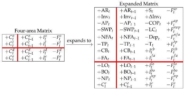 Rows 1–6 represent the operating assets, net of the operating liabilities; rows 7–8 represent to the liquid class; rows 9–11 represent the debt class; row 12 represents the equity class.

A firm or a project may then be described as a system of the above mentioned 12 classes (it is evident that each such class may in turn be disaggregated into further subclasses, further increasing the size of the Matrix). The change in capital depends on income and cash flow. The expanded Matrix contains 12 income components (column 3). Correspondingly, the expanded Matrix contains 12 cash-flow components (column 4). The inner horizonal bar represents equality of the various components. Specifically, column 1 states the following equality:
(same for column 2 with replacing t). Column 3 states the following equality:
while column 4 states the following equality:
Changing signs, the last equality becomes
The SSM (13) simultaneously displays the dynamic evolution of the firm/project and its static equilibrium, expressed in terms of the basic elements of an economic entity: capital, income, and cash flow. Specifically, the four columns describe four equilibrium statements. Respectively,
- an equilibrium statement of financial position for time and time t (columns 1 and 2)
- an equilibrium statement of incomes at time t (column 3)
- an equilibrium statement of cash flow at time t (column 4).
In the next section, we show that the SSM can be managed via a set of working rules (split-screen technique) and that the three above mentioned equilibrium statements are “shapeshifting” financial statements, that is, they may be shaped in many different-but-logically-equivalent ways. The traditional financial statements, namely, the balance sheet (BS), the income statement (IS), and the cash-flow statement (CFS), are but one shape among many possible ones. Reconciliation with traditional financial statements will be based on the split-screen technique. This technique turns the SSM into an effective logical machine which favors accounting and financial analysis and enables a better conceptualization of all the complex relationships among book values, income components, and cash-flow components and, therefore, among BS, IS, and CFS.
4. Mastering the Split-Screen Technique
The split-screen technique consists of performing some simple operations upon the SSM. This technique turns the SSM into a logical device that enables one to effectively manage the labyrinth of intricate relations implied by the three financial statements, as well as easily extract important pieces of accounting information.
We start by highlighting the fact that the expanded Matrix in (13) is disaggregated into upper region (rows 1–8) and lower region (rows 9–12), as well as into left region (column 1) and right region (columns 2–4). Four partitions are then identified: Upper left partition, upper right partition, lower left partition, lower right partition.
Since the inner horizontal and vertical bars denote equality, the sums of the elements of these four partitions coincide. Therefore, mathematically, the SSM is a system of equalities. As such, it enjoys some invariance properties that enable shifting rows and columns by following simple working rules. A set of 8 working rules may be derived. We call the set of the working rules the split-screen technique. The latter enables framing the SSM into different configurations which favor understanding of the relations among variables and help the analyst make complex analysis with no need of mathematical skills nor any accounting or finance background.
Split-screen technique—Working rules
- A row in the upper (lower) region may be shifted downward (upward) to the lower (upper) region, as long as the signs of its elements are changed
- A column in the left (right) region may be shifted to the right (left) region, as long as the signs of its elements are changed
- For any fixed row of the Matrix, the sum of its elements in the left region coincides with the sum of its elements in the right region. This implies that the elements of the opposite partition may be swapped with no change in sign
- For any fixed column of the Matrix, the sum of its elements in the upper region coincides with the sum of its elements in the lower region. This implies that the elements of the opposite partition may be swapped with no change in sign
- Any group of rows (columns) pertaining to the same partition may be consolidated by algebraically summing the respective elements, so reducing the size of the Matrix. Symmetrically, each row may be broken down into further rows, so expanding the size of the Matrix
- The rows (columns) belonging to the upper or lower (left or right) region may be permuted as long as permutation is made within the same partition
- Each cell may be multiplied or divided by the same number.
- Any number may added to any cell , provided that the same number is
- added in any cell in the same row as cell but in the opposite partition, and
- added in any cell in the same column as the cell but in the opposite partition, and
- added in the cell in the same row as cell and in the same column as .
5. Linking the Financial Statements by Means of the Split-Screen Technique
We now reconcile this accounting model based on the SSM with the standard financial statements as can be found in any accounting, finance, or engineering economy text. To do it, we make use of the split-screen technique introduced in the previous section.
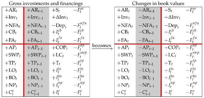
The upper region of the expanded Matrix in (13) shows the net investments. More precisely, it shows the investments in liquid assets and the investments in net operating assets (i.e., operating assets net of operating liabilities). However, the analyst may well be interested in gross investments (i.e., investments before operating liabilities). To this end, we shift rows 3, 4, and 6 down to the lower region while changing the signs of its elements (Rule 1). Therefore,
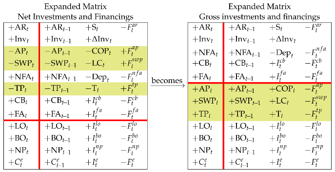 (we remind that whence ). The upper region of the right matrix collects the (gross) investments, consisting of operating investments (rows 1–3) and financial investments (rows 4–5), while the lower region collects the gross financings, divided into operating liabilities (rows 6–8), debt (rows 9–11), and equity (row 12). Column 1 of the right-hand matrix (17) is the traditional Balance Sheet (BS) at time t as can be found in any accounting textbook, whereas column 1 in the left-hand matrix is the traditional BS at time t as can be found in any finance textbook (same for column 2, referred to time ) (see also Figure 3).The composition of the liabilities in the gross-financing structure is referred to as the financial structure.

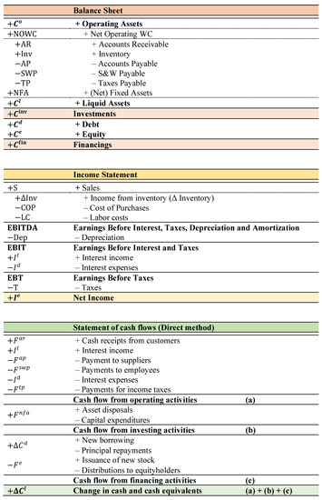
Figure 3.
Traditional Financial Statements.
It is worth noting that (17) supplies a fourfold way of conceptualizing the gross investments: (i) sum of assets (upper left partition), (ii) sum of financings (lower left partition), (iii) sum of start-of-period assets plus the difference between overall income generated by assets and overall cash flow generated by assets (upper right partition), (iv) sum of start-of-period financings plus the difference between overall income accrued to capital providers and overall cash flow distributed to capital providers (lower right partition).
Let us now apply Rule 2 and shift column 2 leftward to the left partition. We get
 We then apply Rule 5 and consolidate columns 1 and 2 of the right-hand matrix and get to a 3-column Matrix, with denoting a change:
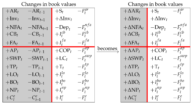 Column 1 of the right-hand Matrix of (19) is a statement of changes in financial position. The four partitions enable the analyst to conceptualize the changes in the book value of assets in four different ways: (i) sum of all the changes in assets (upper left partition), (ii) sum of all the changes in net worth and liabilities (lower left partition), (iii) difference between the income generated by the assets and the cash flow extracted by the assets (upper right partition), (iv) difference between the income accrued to capital providers, employees and Treasury, and the cash flow distributed to capital providers, employees, and Treasury (lower right partition).


We now use Rule 1 to isolate the change in equity as of time t, ; to this end, we shift the operating liabilities and the elements of the debt class upward to the upper region (changing sign) so that
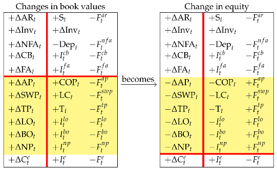 The Change-in-equity Matrix allows one to conceptualize the change in equity in three different terms. The lower right partition uses the law of motion and says that the source of change of equity is net income and cash flow to equity. The upper left partition uses the law of conservation and says that the change in equity is equal to the algebraic sum of the changes in net operating assets (AR, AP, Inv, SWP, NFA, TP), liquid assets (CB, FA), and debt (LO, BO, NP). The upper right partition uses both the law of motion and the law of conservation and describes the change in equity in terms of the income components and cash-flow components of the above mentioned classes (remember that is the inventory income).

We apply Rule 6 to the right Matrix in (20) and reorder the rows of the upper region just to ideally separate the operating area from the financial area (with the tax area kept as the last item):
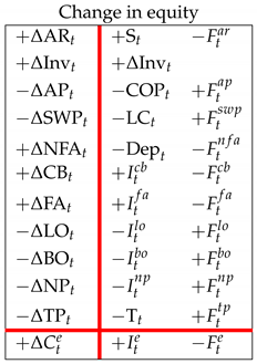 We then use Rule 2 and shift column 3 to the left region in order to isolate the columns reporting the income components:
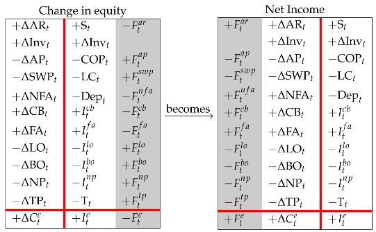 Column 3 in the Net-Income Matrix is nothing but the traditional Income Statement (IS), producing the net income.7 (See also Figure 3). The net income may be conceptualized in terms of (i) income components (upper right partition), (ii) CFE and change in equity (lower left partition), (iii) cash-flow components generated by the operating and non-operating assets, liquid assets, net of CFD plus the algebraic sums of the corresponding book value variations (upper left partition).


Now we show how the traditional cash flow statement is encompassed in the Matrix. This statement may be calculated either with the direct method or with the indirect method. We focus on the direct method, crossreferring to Magni (2020, Section 3.7) for the link with the indirect method. Figure 3 illustrates a standard cash-flow statement with the format of the direct method, as can be found in accounting or finance text (e.g., Williams et al. 2010; Horngren et al. 2012; Weygandt et al. 2012).
We start from Equation (22) (left Matrix) and, for simplicity, we consolidate the debt items (Rule 5), getting to Equation (23) below:
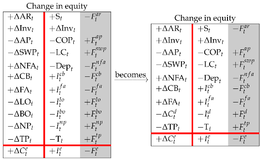 Next, we isolate the cash-flow column by shifting the income column leftward (Rule 2):
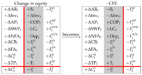 Then, we shift all the rows of the upper partition downward, barring the CB row (Rule 1), so that
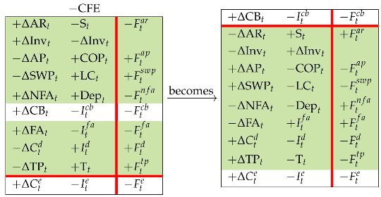 Now we swap the elements of rows 7 and 8 (Rule 3) and consolidate the first two columns (Rule 5), so that
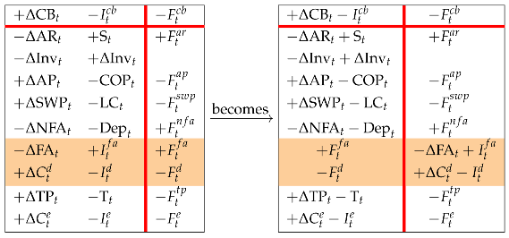 (note that, after consolidation, the number of columns of Matrix (26) is reduced to two). Finally, we apply Rule 8 for adding in rows 1 and 7:
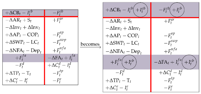 and, hence, swapping the elements of row 1 (Rule 4) and considering that ,
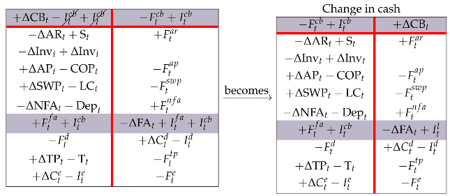 The right region of the Change-in-cash matrix in (28) displays a common cash flow statement. In the following paper (Baschieri and Magni 2023), for the sake of simplicity, we will not break down the liquid assets into CB and FA, so the output of the cash flow statement is the change in cash and cash equivalents (marketable securities and other financial assets). To get to it, one starts from the right matrix in Equation (25) and (i) shifts FA row upward (Rule 1), (ii) consolidates the FA and CB rows (Rule 5), (iii) swaps the elements of the debt row (Rule 3), and (iv) adds in the four partitions (Rule 8). Therefore,
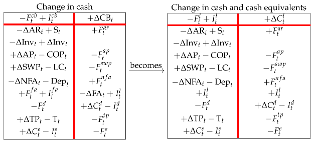 (see also the CFS depicted in Figure 3).


Remark 1.
The cash from operating activities in the traditional statement of cash flows differs from the CFO (). The latter is an operating after-tax cash flow that includes the net capital expenditures (via ) but does not contain interest incomes, , nor financial expenses, , though it does include their tax effect via ). The “cash from operating activities” does not include capital expenditures and includes interest income and interest expenses. The difference between the cash from operating activities in the CFS and the CFO is equal to
6. Costs Classified by Nature or by Function
In the previous sections, we have implicitly classified (pre-tax) operating costs by nature, that is, on the basis of the economic agents to whom the firm owes money: Cost of purchases (suppliers) and cost of labor (employees). The expanded Matrix in (13) is then an expanded Matrix (with accounting values classified) by nature. We now manage the SSM so as to obtain a classification of costs by function, that is, in terms of the process/function that generates them: manufacturing activities or nonmanufacturing activities. The costs generated by the former form the so-called cost of goods sold (COGS); the costs generated by the latter are called selling, general, and administrative costs (SGA).8 The passage from a classification of costs by nature to a classification of costs by function may be obtained by breaking down AP and SWP into further subclasses.
AP is broken down to manufacturing AP and nonmanufacturing AP. The former refers to the accounts payable for manufacturing supplies (direct and indirect material, plant insurance, utilities repair and maintenance, etc.) and nonmanufacturing supplies (office supplies, office insurance, utilities, etc.). We denote it as and , respectively. Correspondingly, the cost of purchases COP, may be broken down into into cost of manufacturing purchases and cost of nonmanufacturing purchases, denoted as and , respectively, and the payments to suppliers, may be broken down to payments for manufacturing supplies and payments for nonmaufacturing supplies, denoted as and , respectively.
Analogously, SWP is broken down to manufacturing SWP and non manufacturing SWP. The former refers to the SWP for manufacturing activities (direct and indirect labor, plant managers’ salaries, etc.), the latter refers to SWP for nonmanufacturing activities (sales and marketing expenses, accounting and administration expenses, delivery expenses, rent expense, executive compensation, etc.). We denote it as and , respectively. Correspondingly, the cost of labor, LC, may be broken down into into manufacturing labor cost and nonmanufacturing labor cost, denoted as and , respectively, and the payments to employees, , may be broken down to payments for manufacturing labor cost and payments for nonmanufacturing labor cost, denoted as and , respectively.
Hence, the law of motion applies:
and
In terms of SSM,
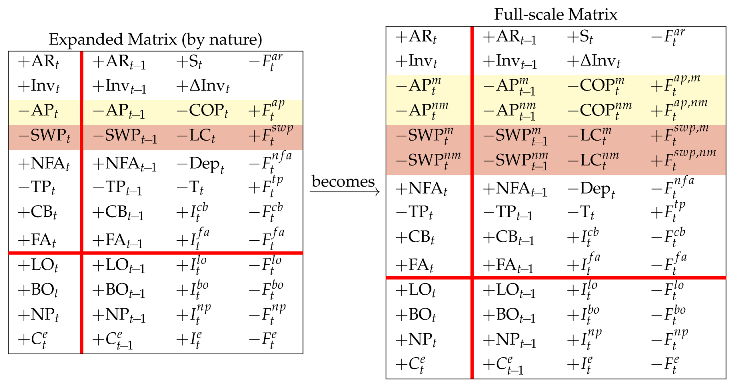 or, in compact form (consolidating the various classes of non-operating assets and debt),
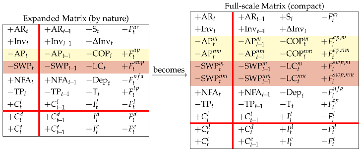 We are now willing to focus on the operating area and sum up all the book values related to manufacturing activities and get what we call the manufacturing Net Operating Liabilities (net of inventories):
Likewise, we sum up the book values related to nonmanufacturing activities and get what we call the nonmanufacturing Net Operating Liabilities:
Same applies with the income components and cash flow components. Specifically, the manufacturing costs, usually called cost of goods sold (COGS), are obtained as
The nonmanufacturing costs, usually called selling, general and administrative expenses (SGA), are obtained as
Same with the cash flows: and with obvious meaning of the symbols. In terms of SSM, we just consolidate the rows related to manufacturing activities and the rows related to nonmanufacturing activities, so that
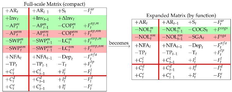 Rows 2 and 3 of the expanded Matrix (by function) describe the law of motion for the manufacturing and nonmanufacturing activities:
The expanded Matrix (by nature) (see left matrix in Equation (33)) and the expanded Matrix (by function) (see right matrix in Equation (36)) are two logically equivalent framings; they are generated by the full-scale Matrix (compact) and report accounting information in different shapes, the former focusing on the nature of the costs and the category of agents which the firm owes the cash payments, the latter focusing on the process which gives rise to the costs and cash flows and the related liabilities (see Figure 4 and Figure 5).


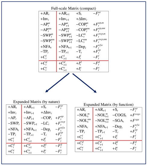
Figure 4.
Expanded Matrices generated by Full-scale Matrix. Expanded Matrix (by nature) is obtained by consolidating the items referring to purchases on one hand and the items referring to labor costs (salaries and wages) on the other hand; Expanded Matrix (by function) is obtained by consolidating the items related to manufacturing activities on one hand and nonmanufacturing activities on the other hand.
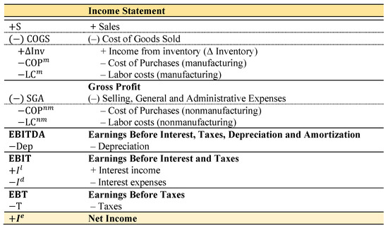
Figure 5.
Income Statement with twofold classification of costs, by nature and by function (see also Figure 4).
We may consolidate and , thereby creating a single class which we call Net Operating Liabilities (NOL):
(note also that ). This class represents an operating liability before (i.e., not considering) taxes payable. We may then rewrite the expanded Matrix (by function) as
 where are the (pre-tax) operating costs and denotes the corresponding payments. Equivalently, consider that
Therefore, we also have
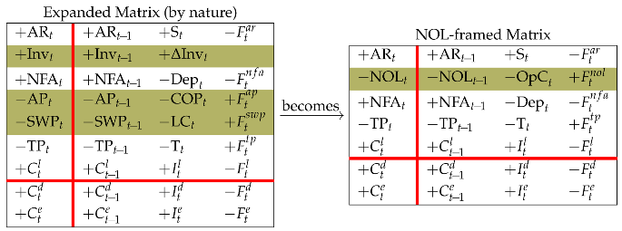 where and . Therefore, the law of motion for NOL (row 2 of NOL-framed Matrix) is
(see also Table 1, Table 2 and Table 3 for the breakdown of NOL, operating costs, and operating payments).


Table 1.
Breakdown of Net Operating Liabilities (adapted from Magni 2020, Table 3.6).

Table 2.
Breakdown of Operating Costs (adapted from (Magni) (2020), Table 3.5).

Table 3.
Breakdown of operating payments.
7. Gross Profit, EBITDA, EBIT, and Net Income
Let us now take the expanded Matrix (by function) and shift rows 3 to 6 down to the lower region (Rule 1) so that


Then, we shift columns 2 and 4 leftward onto the left region (Rule 2), so that


The four partitions describe the Gross Profit (GP), which may then be conceptualized in four different ways:
- -
- upper right partition: the GP is the difference between sales revenues and manufacturing costs (COGS)
- -
- upper left partition: the GP is the difference between the change in AR, net of (change in) manufacturing liabilities, and the cash from customers, net of cash outlays for manufacturing costs
- -
- lower right partition: the GP is the sum of all the costs generated by the firm except the manufacturing ones, plus the income accrued to the capital providers (net income and net interest)
- -
- lower left partition: the GP is the difference between the overall change of the book values of the firm (except AR and manufacturing NOL) and the corresponding cash flows.
In the Gross-profit Matrix, COGS and SGA do not include depreciation charges. Berk and DeMarzo (2014) use the expression “clean expenses” to refer to costs that do not include depreciation charges (see p. 235, footnote 2; see also glossary, p. 1049, and Example 23, p. 266, where COGS is referred to as “Manufacturing expenses (other than depreciation)”. Titman and Martin (2011) use the expressions “operating expenses (before depreciation)” (p. 32) or “operating expenses (excluding depreciation)” (p. 343) to refer to clean SGA. In finance texts, clean COGS and clean SGA are common.
However, depreciation may itself be broken down into a manufacturing component and a nonmanufacturing component, which can be included in the manufacturing costs and nonmanufacturing costs, respectively. Therefore, GP may be redefined as the difference between sales revenues and COGS, including the depreciation of manufacturing assets. To this end, one must split up the NFA and its income and cash-flow components into manufacturing and nonmanufacturing assets, each one fulfilling its own law of motion:
where and represent asset disposals for manufacturing assets and nonmanufacturing assets (net of capital expenditures), so that . The Gross-profit Matrix in (43) may then be reframed:
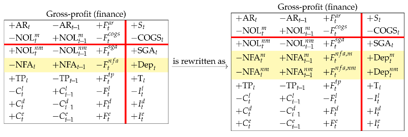 whence, by shifting row 4 to the upper region (Rule 1),
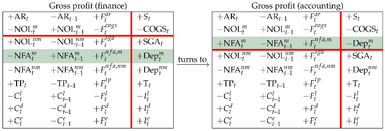 The latter Matrix portraits the GP inclusive of the manufacturing depreciation. The sum of and redefines the cost of goods sold in an accounting perspective. To distinguish the two definitions, we use a circle superscript:
The sum of SGA and redefines the SGA in an accounting perspective:
and are comprehensive COGS and SGA. Comprehensive COGS and SGA are preferred in accounting and engineering economics (e.g., Newnan et al. 2009; Williams et al. 2010; Weygandt et al. 2012; Park 2013), whereas clean COGS and SGA are preferred in corporate finance. Gross profit in an accounting perspective is then equal to
One of the reason for the preference of clean expenses in finance may be that the notion of EBITDA (earnings before interest, taxes, depreciation, and amortization) is felt as particularly important for financial analysis. This notion requires that depreciation should be isolated from other operating costs. In particular, the EBITDA is found from the Gross-profit Matrix in (43) by shifting row 3 up to the upper region (Rule 1):
 The four screens of the EBITDA Matrix supply four ways to conceptualize and calculate the EBITDA.


From (46), we shift row 4 to the upper region to get the EBIT (Rule 1):
 As a result, the SSM may well rationalize two different classifications of operating costs, by nature and by function, as well as all the relationships between the capital components, income components, cash-flow components in either classification, as well as the relation between accounting perspective (comprehensive COGS and SGA) and finance perspective (clean COGS and SGA) (see also Magni 2020, chp. 3). Finally, we show the after-tax operating income, , in four different ways, by shifting the tax row up to the upper region:
 Hence, to get the Net Income, one just has to shift rows 6–7 up to the upper region so that
 which is equivalent to the right Matrix in Equation (22).


8. Working Capital, Net Financial Position, and Operating Cash Flow
A different perspective on assets classifies the operating assets into short-term assets (net operating working capital) and long-term assets (fixed assets). From the NOL-framed Matrix in Matrix (40) we consolidate rows 1, 2, and 4 (Rule 5) to define the net operating working capital (NOWC):
 where is the cash flow associated with NOWC. Then, we shift rows 2 and 3 down to the lower region (Rule 2) to get the NOWC Matrix:
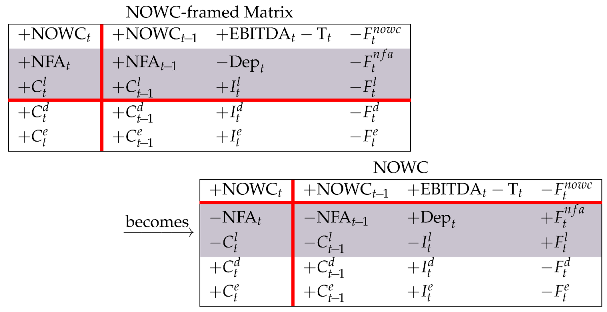 It is then clear that the EBITDA net of taxes is the income component of NOWC.


Shifting row 2 back to the upper region, one gets four ways of modeling the net operating assets (Rule 1):
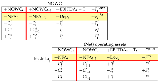 Column 3 of the (net)-operating-assets Matrix depicts the operating income, , from an investment perspective (upper region) and a financing perspective (lower region):
If one consolidates rows 3–4 (Rule 5), one gets
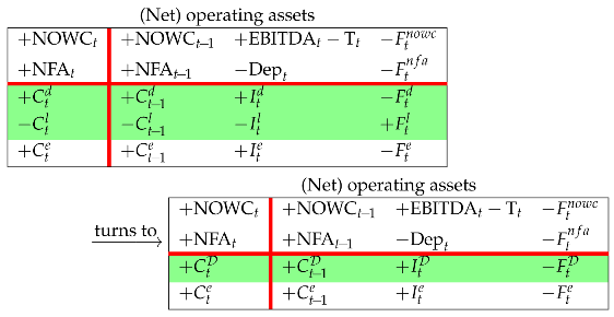 where is the so-called net financial position or net debt, with and being the corresponding income and cash flow components, respectively. The composition of the liabilities in this net-financing structure is referred to as the capital structure (to be distinguished from the financial structure presented in Section 5).


Shifting the equity row up to the upper region (Rule 1) and disaggregating back , one gets four different-but-equivalent ways of calculating the net financial position:
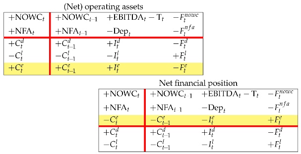 Now, we (i) consolidate back and into (Rule 5), (ii) consolidate the consecutive book values into a BS (Rule 5), (iii) swap the BS column and the CFS column (Rule 2) (iv) shift the equity row down to the lower region (Rule 1), so obtaining four ways to model the operating cash flow (CFO):
 The CFO is sometimes called capital cash flow (see Ruback 1994, 2002).9


9. Free Cash Flow to Equity, Payout Ratio, and Cash Flow from Liquid Assets
The (net) operating assets generate the (after-tax) operating cash flow (CFO). This cash flow is the cash flow (generated by the project in a given period) that is available for distribution to the capital providers (which is precisely the reason why the CFO is often called capital cash flow, CCF). Subtracting the cash flow paid to debtholders from it, one gets the cash flow available for distribution to shareholders, also called potential dividends (PD) or free cash flow to equity (FCFE):
The corresponding capital, , is the amount of capital that would be owned by equityholders if liquid assets were zero. In Matrix format, starting from the four-area Matrix (Equation (12)) and swapping the liquid-area row and the debt row:
 Then, swapping columns 1 and 4, one gets the FCFE:
 From the lower left partition, it derives that the FCFE can also be computed, indirectly, as . If the FCFE is positive, a decision must be made whether to distribute it in full to shareholders or retain part of it as liquid asset (cash or cash equivalents or other marketable securities). This payout decision is often based on a pre-determined payout ratio, , applied to the net income or to the FCFE itself:
Other schemes are possible, including the use of a combination of net income and CFE; for example, the payout ratio may be applied to the minimum between net income and FCFE, as long as they are positive:10
If the FCFE is negative, then it signals a financial deficit and represents the potential contribution by shareholders. The firm must then decide how much of that financial deficit should be contributed by shareholders and how much by withdrawal from liquid assets (or additional debt).11 In this case, is a pay-in ratio.


Therefore, CFE is a decision variable for . At , the project is over and . This means that the whole FCFE is distributed to equityholders,12 along with the balance of the liquid assets:
More simply, since , one can also use
The CFL is the residual amount after the financing decision is made: for . Therefore, a decision on CFE is a decision on CFL as well. The CFL can also be visualized from the FCFE Matrix above by shifting the equity row up to the upper region:
 If is positive (i.e., is negative), it means that part of the operating cash flow is retained by the firm (i.e., not distributed to capital providers) and invested in liquid assets (e.g., cash equivalents or marketable securities); if is zero, then the firm makes a full distribution of the FCFE to equityholders; if is negative (i.e., is positive), the firm distributes more than 100% of the FCFE by withdrawing additional cash flow from the liquid assets.

When appraising a project, the firm must determine, for each year, the payout ratio, which determines the CFE, which, in turn, determines (see CFL Matrix above). The amount is essential, because it enables the analyst to calculate the balance of liquid assets:
The balance of liquid assets is in turn necessary for determining the amount of total assets: . This creates a link between operating variables and decision variables (see also the logical loop described in Magni et al. 2022).
10. Project’s Split-Screen Strip
A project or firm is characterized by a sequence of columns showing the book value, the incomes, and the cash flows. We call this sequence split-screen strip. Two logically equivalent structures stem from the split-screen approach: (i) a sequence of consecutive split-screen Matrices and (ii) three strips of consecutive columns displaying the period evolution of all the book values, the incomes, and the cash flows. We call the latter Transposed Matrix.
10.1. Split-Screen Strip as a Sequence of Consecutive Matrices
Given a set of estimated inputs for the n-period project, n split-screen Matrices can be built, one for each period. This implies that there exists a strip of n split-screen Matrices describing the project’s pro forma financial statements, which may be placed side by side:
 or, equivalently, swapping left and right region (Rule 3),
 The above strip, presented in Magni (2020, Section 12.2), does not easily lend itself to spreadsheet modeling. Since we are interested to apply the split-screen approach to spreadsheet modeling in the following paper (Baschieri and Magni 2023), we introduce a refinement of it, which turns out to be essential for modeling purposes. Specifically, we merge all the Matrices by overlapping the last and first column of any two consecutive Matrices, so that one may write this reframe the sequence of snapshots as a single, continuous strip:13
 where for and with the understanding that the convention on the meaning of the vertical bar (now in Indian red) is changed as follows: for each row, the sum of the three elements preceding the bar (capital at time t−1, income at time t, and cash flow at time t) is equal to the element following the bar (capital at time t).


In terms of the full-scale Matrix (Equation (36), left matrix), the full-scale strip becomes
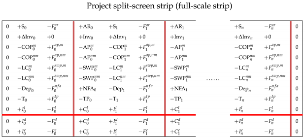 (The system moves from a zero level at and ends up at zero level at ).

10.2. The Transposed Matrix
Abstracting from the sign, in the four-area strip, the columns of book values, incomes, and cash flows are placed horizontally, one after the other:
 for . A different representation of the project is obtained by transposing the layout of (69) from horizontal to vertical and, considering that there are as many columns as there are periods, one gets three strips of capital, income, and cash flow representing the project’s split-screen strip:
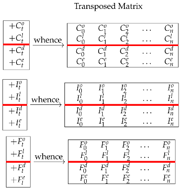 The three strips represent three submatrices. Taken together, they represent what we call the Transposed Matrix; it gives a different-but-equivalent layout, which visualizes, horizontally, the period sequence of all the book values, the incomes, and the cash flows and, vertically, the law of conservation.


11. Benchmark Matrix, Economic Value, and the WACC
Once the project split-screen strip has been built, one needs appraise the project. To this end, consider a replicating portfolio with the expected cash flow at time (same prospective cash flows as the project’s) and assume it is comparable in risk to the project’s. We call this the benchmark portfolio. As seen in Section 2, the law of motion holds for any asset; therefore, it holds for the benchmark portfolio as well. Then, letting be its expected rate of return and its market value,
where . Equation (71) may be written as
where is the (expected) profit of the benchmark portfolio. Equation (71) may also be written, in a backward fashion, as
Using backward induction on it, starting from , and reminding that for , one gets
and, if is time-invariant,
The value is the amount that any investor should invest to purchase the benchmark portfolio. This is also called the economic value or intrinsic value of the project.14 Equation (74) formalizes the so-called time-value-of-money principle, according to which the economic value of any asset is the sum of its prospective cash flows discounted at .
The expected return on the benchmark asset represents the required return on the project’s assets (i.e., the minimum attractive rate of return for the capital providers). From an investment perspective, the benchmark portfolio may be viewed as an investment benchmark portfolio; from a financing perspective, the benchmark portfolio may be viewed as a financing benchmark portfolio. The former consists of two financial assets: an asset replicating the prospective CFOs, (i.e., for, ) and an asset replicating the prospective CFLs, (i.e., for ), whereas the latter consists of an asset replicating the prospective CFDs, (i.e., for ) and an asset replicating the prospective CFEs, (i.e., for ). Since , the value of the investment benchmark portfolio and the financing benchmark portfolio coincide. This expresses the law of conservation for the benchmark portfolio:15
where
Practically, the economic value of equity is more conveniently calculated from the other three economic values as (see Baschieri and Magni 2023, Section 4.1).
The left-hand side of (76) supplies the price of the investment benchmark portfolio and the right-hand side supplies the price of the financing benchmark portfolio. Such prices represent, by definition, the economic values of the firm’s assets and firm’s net worth and liabilities, respectively.
Given that the law of conservation holds for both economic values and cash flows, then (76) also implies the law of conservation for the benchmark profits (market returns):
where , , is the expected rate of return on the respective benchmark asset.16 Hence, in terms of SSM, the project Matrix may be matched by a corresponding benchmark Matrix having the same cash flows from to (but different profits and capital values):
 (where for ) or, equivalently,
 where
denotes the benchmark profit. The two Matrices in (78) share the same logic and the same structure but differ in values: The project Matrix uses book values () and accounting profits (), whereas the benchmark Matrix uses economic (or intrinsic) values () and economic profits (). Columns 1 and 2 of the benchmark Matrix say that the economic value of investments at a given date equals the economic value of financings. Column 3 expresses the law of conservation for benchmark profits and gives rise to the notion of weighted average cost of capital (WACC). More precisely, shifting row 2 of the benchmark Matrix down to the lower region and consolidating liquid assets and debt in (78), one gets
 where is the economic value of the net debt and is the required return on net debt. Consolidating the last two rows,
 Dividing each cell of (82) by (Rule 7), one gets
 Shifting columns 2 and 4 onto the left side, one gets the (pre-tax) WACC Matrix, expressing the WACC in four different ways:
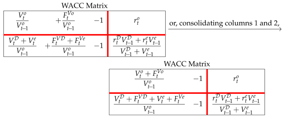 Column 3 of the right Matrix in (84) says that the (pre-tax) WACC is equal to the weighted mean of the required return on equity and the required return on net debt:
which is the usual definition in finance.17


The Transposed Matrix can be built for the benchmark as well. It is equivalent to Equation (70) with economic values replacing book values:
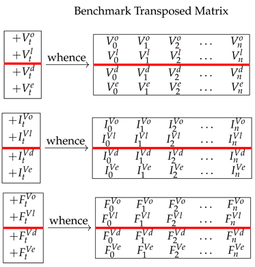 As we will see in the following paper (Baschieri and Magni 2023), the project Transposed Matrix and the benchmark Transposed Matrix are particularly helpful formats when evaluating the project via spreadsheets.

12. Project Appraisal: Net Present Value and Residual Income
A project is entirely described dynamically and statically by its strip of split-screen Matrices. Likewise, there exists a strip of n split-screen Matrices (the benchmark’s split-screen strip completely describing the benchmark portfolio:
 where
where

- for and for
- for
- ,
with . Matching the project split-screen strip and the benchmark split-screen strip, the notion of market value added (MVA) and net present value (NPV) arise. More precisely, let us focus on the two matrices in (78). Subtracting each element of the left-hand matrix (book values) from the elements of the right-hand matrix (economic values), one gets the following MVA matrix:
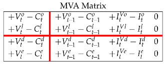 where is the MVA for area . For , the MVA is called net present value (NPV):
The project NPV can be viewed as the sum of the operating NPV and non-operating NPV (investment perspective) or the sum of debt NPV and equity NPV:
The project NPV expresses the value created by the project, which is captured by the capital providers (debtholders and equityholders). The equity NPV is the shareholder value created, which is captured by the equityholders:
The project is worth undertaking if and only if it creates value for the firm’s shareholders, that is, if . Usually, finance scholars and practitioners assume that the nominal value of debt is equal to the economic value of debt: for all t, which implies , which in turn implies so that the decision criterion may also be stated in terms of project NPV instead of equity NPV: the project is worth undertaking if and only if .

Economic profitability may also be expressed in terms of incomes. Specifically, the difference between the project income and the benchmark profit expresses the income over and above the benchmark profit. We call it Economic Residual Income (ERI. See Magni 2021a):
The amount quantifies the profit over and above the benchmark profit for each of the four areas in a given period t. Using the acronyms, one can rewrite (88) as
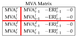 The third column of (91) says that the sum of the operating ERI and non-operating ERI is precisely equal to the project’s ERI and equal to the sum of the debt ERI and equity ERI:
In other words, ERI is unambiguous under both an investment perspective (left-hand side) and a financing perspective (right-hand side). This is by no means a trivial fact: contrary to the ERI, the standard notion of residual income, as found in finance and accounting, is non-additive and, as such, it is economically unreliable.18

There exists a sequence of n such MVA Matrices, whence the MVA split-screen strip:
 It is natural to believe that the sum of the ERIs generated in the project’s lifespan provides a measure of the project’s economic profitability. This is true, since the MVA Matrix says
Iterating, and considering that ,
(we omit the superscript j for convenience). Since , then
In other words, the stream of the ERIs perfectly decomposes the NPV, providing information on the way economic value is created through time.

13. Measuring Economic Profitability and Making Decisions
In the previous section, we have introduced the NPV and the related criterion. In this section, we present four other measures of worth that stem directly from the split-screen strips and present the decision criterion associated with each measure. All the five decision criteria are reciprocally consistent and provide different-but-logically equivalent information about the project’s economic profitability.
- (1)
- Total ERI. We define the Total ERI as the sum of all the ERIs:with and . The total ERI is an absolute measure of worth, expressed in terms of incomes: it expresses the total above-normal profit generated by the project in its lifespan.
- (2)
- Average ERI. Summing all the incremental profits through the incremental matrices and dividing by the project’s duration, one gets the the average incremental profit (AERI):It expresses a fundamental earning power of the project, that is, the ability of the project of providing profits over and above the benchmark profit that could be obtained by investing in an equivalent-risk benchmark asset. It is an absolute measure of worth, referred to a single (average) period.
- (3)
- Cash-flow return on capital. Consider the cash-flow vector and the book value vector . Summing all the cash flows , one gets the total cash flow generated by the project, denoted as F. Summing all the capital amounts , one gets the total investment, denoted as C. Dividing the former by the latter, one gets the cash-flow return on capital (CFROC):An analogous CFROC is available for the benchmark portfolio. The cash-flow vector is, in this case, . Therefore, the benchmark CFROC isand are relative measure of worth, which quantifies the net cash flow generated, respectively, by the project and the benchmark, as measured per unit of total capital committed, C.19 The difference between is a measure of financial efficiency: it measures the cash-flow return of the project over and above the benchmark cash-flow return.
- (4)
- Rate of return. Let be the project’s income vector. Summing all the components of , one gets the total profit generated by the project, denoted as I. Dividing it by the total invested capital C, one gets the project’s rate of return:(If the total investment C is zero, we define i to be if or if .) The project rate of return in (99) has the following features:
(1) it is an average rate of return (total return to total capital)
(2) it is an internal return rate, that is, it does not depend on the COC/MARR
(3) it is an accounting rate of return (use of pro forma accounting profits and book values)
This rate of return is also known as Internal Average Rate of Return (IARR) (see Magni 2021b, for a detailed treatment).
Note that the IARR is much easier to understand (just a return divided by a capital amount) as compared with the traditional Internal Rate of Return (IRR), which is the solution of an equation. Regarding the latter, which is taught in any business school and widely employed in real life, its unreliability is well-known in the literature long since (see, e.g., Hirshleifer 1958; Bailey 1959; Teichroew et al. 1965a, 1965b). In particular, the IRR may not exist or multiple IRRs may arise.20 In contrast, the IARR has the following feature:
(4) it exists and is unique.21
An analogous rate of return is available for the benchmark investment. The benchmark profit’s vector is . Summing all the components of , one gets the total profit generated by the benchmark, denoted as . Dividing by the total invested amount, C, one gets the benchmark return
This is an average rate of return, quantifying the total foregone profit per unit of capital invested in the project. The rates i and are relative measures of worth and the difference is a measure of financial efficiency, that is, it quantifies the project’s average profit over and above the profit expected from the benchmark investment. In other words, if the firm undertakes the project, the capital providers earn a total i on a total amount C, but, at the same time, forego to earn a total on the same amount. The differences signal values creation (if positive) or destruction (if negative).
Given that there are four classes (operating, non-operating, debt, equity), there is one such measure for each class. The project should be undertaken if shareholders’ wealth will be increased, as opposed to the benchmark investment. We have seen that, in terms of NPV, this means that the project should be undertaken if . In terms of the metrics presented in this section, we have the following accept-reject criteria.
Total ERI criterion. The project creates value and is worth undertaking if and only if the total equity ERI is greater than zero:
Average ERI criterion. The project creates value and is worth undertaking if and only if the average equity ERI is greater than zero:
CFROC criterion. The project creates value and is worth undertaking if and only if the equity CFROC is greater than the benchmark CFROC:
Rate-of-return criterion. The project creates value and is worth undertaking if and only if the equity rate of return is greater than the corresponding COC:
In the latter two criteria, if , then the condition for acceptance is reversed, for the project is a borrowing project. (See Lima e Silva et al. 2018 for details.)
If the project is unlevered (i.e., for all t) or if and for all t, as is (often unawarely) assumed in the finance and engineering practice, then the use of the project NPV or the equity NPV is equivalent:
Likewise, the four above mentioned measures of worth may be used in either a project perspective or an equity perspective: the decision recommendation will be the same.
It is easy to see that the decision criteria presented are indeed consistent one another (they lead to the same decision): it suffices to show that they are all NPV-consistent.
The NPV-consistency of all the proposed measures holds because the NPV can also be expressed in the following ways (we omit the superscript e for sake of convenience):
The proof is simple. First, the total ERI is equal to the NPV by (95). Therefore, and and, hence, . Also, since and (as is easily proved), then and , which proves that .
Such a consistency of the five criteria may be employed by the modeler not only for extracting information about absolute and relative economic profitability, but also as a check of the internal consistency of the model.
Remark 2.
The rate () acts as the MARR for the project. It is a cutoff rate which signlas value creation or value creation. If , then if , the project is worth udndertaking (assuming ). It is easy to show that (see Lima e Silva et al. 2018, chp. 10 and Magni 2021b); that is, is just a modified cost of capital, to take account of the fact that the capital invested in the benchmark is different from the capital invested in the project. The factor make r comparable with i.
Remark 3.
As anticipated, the use of the equity perspective or the project perspective for decision-making is immaterial if the project is not financed with debt nor liquid assets or if the nominal values of debt and liquid assets are equal to their economic values. Focusing on rates of return, the project rate of return, i is an average Return On Assets (ROA) while the equity rate of return, , is an average Return On Equity (ROE). Under an investment perspective, the average ROA is the weighted mean of the average ROI (return on operating investment, ) and average ROL (return on liquid assets, ). Under a financing perspective, the project rate of return is an average return on financings. It is the weighted mean of the average ROE (return on equity, ) and the average ROD (return on debt, ) with obvious meanings of and , . For the law of conservation of incomes and capitals, the average return on financings is also equal to the average ROA. An analogous line of reasoning works for the MARRs as well (see Table 4). (See also Magni 2020, chp. 10 and Magni 2021b for more details).In finance, the notions of COC and MARR coincides. However, in real-life applications, many firms use hurdle rates which differ from the normative COC. The hurdle rate is a cutoff rate that identifies a MARR that decision makers fix using subjective evaluations, which may or may not involve the calculation of market-determined risk premiums. We assume the MARR is an input parameter (see McDonald 2000; Jagannathan and Meier 2002; Magni 2009a; and Magni 2020, Section 5.6, on the use of heuristics for selecting a MARR) and, for simplicity, we assume that is constant across periods (see Magni 2021a, 2021b for a generalization to time-varying rates).

Table 4.
Link among NPV, rate of return and benchmark rate of return.
The financial efficiency of the project is while the financial efficiency of the equity investment is . The latter expresses the appropriate excess return for decision-making, while the former can be used only insofar as the project is not financed with debt or the return on debt is equal to the required return on debt.22
Remark 4.
The last two equations in (102) provide an intriguing product structure: the NPV is decomposed into a scale factor (total invested capital) and a financial-efficiency factor (rate of return): . This breakdown enables the analyst to appreciate the contribution of the investment scale (C) as opposed to the ability of the project of generating above-normal returns (). A further breakown is possibile, apportioning the scale factor and the efficiency factor to the various areas:
With the calculation of the project’s economic profitability and shareholder value creation, the AFES is completed.
14. Spreadsheet Modeling
The adoption of the SSM and the use of a continuous split-screen strip, with merged columns, makes the AFES particularly suited for spreadsheet modeling. It is put to full use in the next paper (Baschieri and Magni 2023). In it, we show that the AFES lends itself to be translated onto spreadsheets in a simple and user-friendly way, with no use of the traditional financial functions and the only use of the INDEX() and MATCH() functions. In Baschieri and Magni (2023), we start from the informal description of the project and describes the AFES by breaking the modeling process down to 7 modules:
- Module 1: Extracting the data of the project
- Module 2: Building the project split-screen strip
- Module 3: Building the strips of other matrix representations
- Module 4: Building the benchmark split-screen strip
- Module 5: Performing the single-period analysis
- Module 6: Reshaping the project split-screen strip
- Module 7: Assessing value creation and financial efficiency.
For each module, we provide a detailed guide with all the necessary steps to complete it and the crossreferences to this paper.
The file with the spreadsheet model can be downloaded at https://morespace.economia.unimore.it/carloalbertomagni/spreadsheet-modeling/ (accessed 18 February 2023) or requested to magni@unimo.it.
15. Conclusions
We describe an innovative approach for modeling capital asset investments, the accounting-and-finance engineering system (AFES), developed in Magni (2020), and show that it favors the whole modeling process via the use of a split-screen approach, according to which the input data are gathered and processed in a structured matrix environment (the split-screen Matrix). The complex network of accounting and financial relations are easily grasped with the project Matrix, which embeds the project’s pro forma balance sheets, income statements, cash flow statements in the same visual representation, making the relations among the various statements clear and easy to grasp.
To evaluate the project and assess value creation, a benchmark split-screen strip is built, which describe the economic values and the benchmark profit that is foregone by the investors in case of project undertaking.
The use of the continuous split-screen strips for the project and the benchmark greatly simplifies spreadsheet modeling. In particular, matching the project split-screen strip (containing accounting magnitudes) against the benchmark split-screen strip (containing economic magnitudes), the resulting Market Value Added strip is generated, which provides several measures of worth (net present value, average economic residual income, average rate of return, cash flow return on capital) that consistently determine the project acceptability and quantify the economic value created in different ways.
Another important feature of the AFES is that it supplies several ways for spotting modeling errors and inconsistencies, so it also acts as a diagnostic tool for removing internal model inconsistencies.
The second part of the AFES presentation (Baschieri and Magni 2023) shows how to put the AFES to full use. The reader will then be able to appreciate that this logical system is particularly useful for spreadsheet modeling and analysis and implementation in real-world application.
Funding
This research received no external funding.
Institutional Review Board Statement
Not applicable.
Informed Consent Statement
Not applicable.
Data Availability Statement
The spreadsheet model is freely available on the Internet at https://morespace.economia.unimore.it/carloalbertomagni/spreadsheet-modeling/ (accessed 18 February 2023). It can also be obtained by writing to magni@unimo.it or d.baschieri@grafspa.it.
Conflicts of Interest
The author declares no conflict of interest.
Notes
| 1 | By “financing policy’ we mean the decisions about how to cover the financial need triggered by the project and the decisions about the amount of cash retained and the amount of cash distributed to equityholders (also known as payout policy or distribution policy.) | ||||||||
| 2 | For example, if , then | ||||||||
| 3 | The primary surplus/deficit is the difference between tax revenues and government spending. | ||||||||
| 4 | A project may be conceptualized itself as a firm; it is an incremental firm which is added to the original firm (or subtracted, in case of abandonment projects). | ||||||||
| 5 | Note that additional borrowing at time t is included in . If the amount of the new borrowing exceeds the instalments paid on the existing loans, then will be negative. | ||||||||
| 6 | For example, if book value of assets at time is $800, depreciation at time t is $20, capital expenditures at time t are $50, and disposal of assets at time t is $60, then . | ||||||||
| 7 | The last item of the income statement refers to the income taxes, . To calculate them, one simply applies the tax rate, , to the higher-level items, which constitute the Earnings Before Taxes (EBT):
| ||||||||
| 8 | This classification is particularly widespread in applied corporate finance and in engineering economics and, in general, whenever dealing with industrial firms. | ||||||||
| 9 | The capital cash flow (or cash flow from operations) should not be confused with the free cash flow (FCF), which is equal to the capital cash flow netted out of tax shield:
Capital cash fow and FCF coincide if the firm is unlevered or if the tax rate is zero. See Magni (2020, Sections 4.7–4.11) for the FCF Matrix and detailed relations between and FCF. Analogously, the FCF should not be confused with the FCFE:
| ||||||||
| 10 | In Baschieri and Magni (2023), we consider two alternative different payout policies. | ||||||||
| 11 | Use of liquid assets to finance projects is common for firms with a substantial amount of liquid assets or for small firms, which rarely make recourse to issuance of new shares. | ||||||||
| 12 | Time n is, by definition, the time where all the (direct and indirect) cash flow effects of the project cease, so may be interpreted as a liquidation dividend. | ||||||||
| 13 | Section 3 in Baschieri and Magni (2023) shows that such a merging greatly facilitates the construction of all pro forma financial statements in a spreadsheet, starting from the estimated input parameters and only using the MATCH and INDEX functions. | ||||||||
| 14 | Put another way, the economic value of a project is “the price the project would have if it were traded” (Mason and Merton 1985, pp. 38–39). | ||||||||
| 15 | This is but the well-known law of one price. See Berk and DeMarzo (2014), (Magni 2020, Section 5.1) or any finance textbook (see also Varian 1987 for the related concept of arbitrage). | ||||||||
| 16 | These expected rates of return are also called required returns:
| ||||||||
| 17 | Note that is a pre-tax WACC. Applying the time-value-of-money principle (i.e., Equation (74)) to and , one finds the economic value of the operating assets (see Ruback 1994, 2002; Fernández 2002; Tham and Vélez-Pareja 2004):
| ||||||||
| 18 | Residual income, or excess profit, is traditionally defined as (see, e.g., Edwards and Bell 1961; Bodenhorn 1964; Peasnell 1981, 1982; Brief and Peasnell 1996; Ohlson 1989, 1995, 2003; Magni 2009b). This definition does not comply with value additivity, a basic tenet in finance (see, e.g., Varian 1987) and a necessary property for reliable financial analysis. In particular, a project’s residual income is not equal to sum of the residual operating income, , and residual interest income, :
Analogously, from a financing perspective, a project’s residual income is not equal to the sum of the residual net income and residual financial expense: , with obvious meaning of the symbol. This problem is entirely solved with the ERI, which makes use of economic value, , in place of book values, , as evidenced by (92) (see also Magni 2020 and, especially, Magni 2021a for details on non-additivity of the standard residual income and the ERI notion). | ||||||||
| 19 | By undertaking the project, the firm’s shareholders forego the opportunity of investing in the benchmark portfolio and get the same prospective cash flows as the project’s: is the rate of return of such a foregone investment. | ||||||||
| 20 | For real-life projects with no IRR, see Lima e Silva et al. (2018); Baschieri et al. (2020); and Marchioni et al. (2020). | ||||||||
| 21 | As a matter of fact, the IRR suffers from many other pitfalls, none of which involves the IARR. For a detailed treatment of such pitfalls we refer the reader to Magni (2013), where 18 problems of the IRR are described, and to Magni (2020, chp. 9), where numerous examples are presented where IRR fails. (See also Hazen 2003 and Hartman and Schafrick 2004). | ||||||||
| 22 | In engineering texts as well as in finance texts, the (often unstated or even unaware) assumption is precisely that for all t. This may well hold or not hold, so care must be taken in selecting the perspective. |
References
- Bailey, Martin J. 1959. Formal criteria for investment decisions. Journal of Political Economy 67: 476–88. [Google Scholar] [CrossRef]
- Baschieri, Davide, and Carlo Alberto Magni. 2023. The split-screen approach for project appraisal (Part II: Spreadsheet Modeling). Journal of Risk and Financial Management 16: 157. [Google Scholar]
- Baschieri, Davide, Carlo Alberto Magni, and Andrea Marchioni. 2020. Comprehensive financial modeling of solar PV systems. Paper prestented at the 37th European Photovoltaic Solar Energy Conference and Exhibition (EU PVSEC), Online, September 7–11. [Google Scholar]
- Berk, Jonathan, and Peter DeMarzo. 2014. Corporate Finance, 3rd ed. (global ed.). Harlow: Pearson. [Google Scholar]
- Bodenhorn, Diran. 1964. A cash-flow concept of profit. Journal of Finance 19: 16–31. [Google Scholar]
- Brealey, Richard A., Stewart C. Myers, and Franklin Allen. 2019. Principles of Corporate Finance, 13th ed. New York: McGraw-Hill Irwin. [Google Scholar]
- Brief, Richard P., and Kenneth V. Peasnell, eds. 1996. Clean Surplus: A Link Between Accounting and Finance. New York and London: Garland Publishing. [Google Scholar]
- Edwards, Edgar O., and Philip W. Bell. 1961. The Theory and Measurement of Business Income. Berkeley: Berkeley University of California Press. [Google Scholar]
- Ehrhardt, Michael C., and Eugene F. Brigham. 2016. Corporate Finance. A Focused Approach. Boston: Cengage Learning. [Google Scholar]
- Feltham, Gerald A., and James A. Ohlson. 1995. Valuation and clean surplus accounting for operating and financial activities. Contemporary Accounting Research 11: 689–731. [Google Scholar] [CrossRef]
- Fernández, Pablo. 2002. Valuation Methods and Shareholder Value Creation. San Diego: Elsevier Science. [Google Scholar]
- Damodaran, Aswath. 1999. Applied Corporate Finance. A User’s Manual. New York: Wiley. [Google Scholar]
- Damodaran, Aswath. 2006. Damodaran on Valuation. Security Analysis for Investment and Corporate Finance. Hoboken: Wiley. [Google Scholar]
- Hartman, Joseph C. 2007. Engineering Economy and the Decision-Making Process. Upper Saddle River: Pearson. [Google Scholar]
- Hartman, Joseph C., and Ingrid C. Schafrick. 2004. The relevant internal rate of return. The Engineering Economist 49: 139–58. [Google Scholar] [CrossRef]
- Hazen, Gordon B. 2003. A new perspective on multiple internal rates of return. The Engineering Economist 48: 31–51. [Google Scholar] [CrossRef]
- Hirshleifer, Jack. 1958. On the theory of optimal investment decision. Journal of Political Economy 66: 329–52. [Google Scholar] [CrossRef]
- Horngren, Charles T., Walter T. Harrison, and M. Suzanne Oliver. 2012. Financial and Managerial Accounting, 3rd ed. Upper Saddle River: Pearson. [Google Scholar]
- Jagannathan, Ravi, and Iwan Meier. 2002. Do we need CAPM for capital budgeting? Financial Management 31: 55–77. [Google Scholar] [CrossRef]
- Lima e Silva, Jessica, Vinicius Amorim Sobreiro, and Herbert Kimura. 2018. Pre-purchasing financing pool: Revealing the IRR problem. The Engineering Economist 63: 193–217. [Google Scholar]
- Magni, Carlo Alberto. 2009a. Investment decisions, net present value and bounded rationality. Quantitative Finance 9: 967–79. [Google Scholar] [CrossRef]
- Magni, Carlo Alberto. 2009b. Splitting up value: A critical review of residual income theories. European Journal of Operational Research 198: 1–22. [Google Scholar] [CrossRef]
- Magni, Carlo Alberto. 2013. The internal-rate-of-return approach and the AIRR paradigm: A refutation and a corroboration. The Engineering Economist 58: 73–111. [Google Scholar] [CrossRef]
- Magni, Carlo Alberto. 2020. Investment Decisions and the Logic of Valuation. Linking Finance, Accounting, and Engineering. Cham: Springer. [Google Scholar]
- Magni, Carlo Alberto. 2021a. Economic profitability and (non)additivity of residual income. Annals of Finance 17: 471–99. [Google Scholar] [CrossRef]
- Magni, Carlo Alberto. 2021b. Internal rates of return and shareholder value creation. The Engineering Economist 66: 279–302. [Google Scholar] [CrossRef]
- Magni, Carlo Alberto, Andrea Marchioni, and Davide Baschieri. 2022. Impact of financing and payout policy on the economic profitability of solar photovoltaic plants. International Journal of Production Economics 244: 108338. [Google Scholar] [CrossRef]
- Marchioni, Andrea, Carlo Alberto Magni, and Davide Baschieri. 2020. Investment and financing perspectives for a solar photovoltaic project. Presented at the Management International Conference (MIC 2020), Ljubljana, Slovenia, November 12–15. [Google Scholar]
- Mason, Scott P., and Robert C. Merton. 1985. The role of contingent claims analysis in corporate finance. In Recent Advances in Corporate Finance. Edited by Edward I. Altman and Marti G. Subrahymanyam. Boston: Irwin. [Google Scholar]
- McDonald, Robert L. 2000. Real options and rules of thumb in capital budgeting. In Project Flexibility Agency and Competition: New Developments in the Theory and Application of Real Options. Edited by Brennan Michael Joseph and Trigeorgis Lenos. New York: Oxford University Press. [Google Scholar]
- Newnan, Donald G., Ted G. Eschenbach, and Jerome P. Lavelle. 2009. Engineering Economic Analysis, International 10th ed. Oxford: Oxford University Press. [Google Scholar]
- Ohlson, James A. 1989. Accounting earnings, book values, and dividends: The theory of the clean surplus equation in equity valuation. Unpublished manuscript (Reprinted in Brief R, Peasnell KV (Eds.) 1996. In Clean Surplus. A Link Between Accounting and Finance. New York: Garland. [Google Scholar]
- Ohlson, James A. 1995. Earnings, book values, and dividends in equity valuation. Contemporary Accounting Research 11: 661–87. [Google Scholar] [CrossRef]
- Ohlson, James A. 2003. Positive (zero) NPV projects and the behavior of residual earnings. Journal of Business Finance and Accounting 30: 15–37. [Google Scholar] [CrossRef]
- Park, Chan S. 2013. Fundamentals of Engineering Economics, International ed. Harlow: Pearson. [Google Scholar]
- Peasnell, Ken V. 1981. On capital budgeting and income measurement. Abacus 17: 52–67. [Google Scholar] [CrossRef]
- Peasnell, Ken V. 1982. Some formal connections between economic values and yields and accounting numbers. Journal of Business Finance and Accounting 9: 361–81. [Google Scholar] [CrossRef]
- Ross, Stephen A., Randolph Westerfield, and Bradford D. Jordan. 2011. Essentials of Corporate Finance, 7th ed. New York: McGraw-Hill/Irwin. [Google Scholar]
- Ross, Stephen A., Randolph W. Westerfield, and Jeffrey F. Jaffe. 2013. Corporate Finance, 7th ed. New York: McGraw-Hill/Irwin. [Google Scholar]
- Ruback, Richard S. 1994. A Note on Capital Cash Flow Valuation. Harvard Business School Background Note 295-069, November. (Revised January 1995). Available online: https://www.hbs.edu/faculty/Pages/item.aspx?num=7567 (accessed on 18 February 2023).
- Ruback, Richard S. 2002. Capital cash flows: A simple approach to valuing risky cash flows. Financial Management 31: 85–103. [Google Scholar] [CrossRef]
- Teichroew, Daniel, Alexander A. Robichek, and Michael Montalbano. 1965a. An analysis of criteria for investment and financing decisions under certainty. Management Science 12: 151–79. [Google Scholar] [CrossRef]
- Teichroew, Daniel, Alexander A. Robichek, and Michael Montalbano. 1965b. Mathematical analysis of rates of return under certainty. Management Science 11: 395–403. [Google Scholar] [CrossRef]
- Tham, Joseph, and Ignacio Vélez-Pareja. 2004. Principles of Cash Flow Valuation. Burlington: Elsevier Academic Press. [Google Scholar]
- Titman, Sheridan, and John Martin. 2011. Valuation. The Art and Science of Corporate Investment Decisions, 2nd ed. Boston: Pearson. [Google Scholar]
- Varian, Hal R. 1987. The arbitrage principle in financial economics. Journal of Economic Perspectives 1: 5–72. [Google Scholar] [CrossRef]
- Welch, Ivo. 2009. Corporate Finance. An Introduction. Boston: Pearson Education. [Google Scholar]
- Weygandt, Jerry J., Paul D. Kimmel, and Donald E. Kieso. 2012. Accounting Principles, 10th ed. Hoboken: John Wiley & Sons, Inc. [Google Scholar]
- Williams, Jan R., Susan Frances Haka, Mark S. Bettner, and Joseph V. Carcello. 2010. Financial and Managerial Accounting. The Basis for Business Decisions, International ed. New York: McGraw-Hill. [Google Scholar]
Disclaimer/Publisher’s Note: The statements, opinions and data contained in all publications are solely those of the individual author(s) and contributor(s) and not of MDPI and/or the editor(s). MDPI and/or the editor(s) disclaim responsibility for any injury to people or property resulting from any ideas, methods, instructions or products referred to in the content. |
© 2023 by the author. Licensee MDPI, Basel, Switzerland. This article is an open access article distributed under the terms and conditions of the Creative Commons Attribution (CC BY) license (https://creativecommons.org/licenses/by/4.0/).