Article

Modeling the Optimal Combination of Proportional and Stop-Loss Reinsurance with Dependent Claim and Stochastic Insurance Premium

Faculty of Mathematics and Natural Sciences, Institut Teknologi Bandung, Bandung 40132, Indonesia
*
Author to whom correspondence should be addressed.
J. Risk Financial Manag. 2023, 16(2), 95; https://doi.org/10.3390/jrfm16020095
Submission received: 31 December 2022 / Revised: 23 January 2023 / Accepted: 2 February 2023 / Published: 6 February 2023

Abstract

:
This paper investigates an optimal reinsurance policy using a risk model with dependent claim and insurance premium by assuming that the insurance premium is random. Their dependence structure is modeled using Sarmanov’s bivariate exponential distribution and the Farlie–Gumbel–Morgenstern (FGM) copula-based bivariate exponential distribution. The reinsurance premium paid by the insurer to the reinsurer is fixed and is charged by the expected value premium principle (EVPP) and standard deviation premium principle (SDPP). The main objective of this paper is to determine the proportion and retention limit of the optimal combination of proportional and stop-loss reinsurance for the insurer. Specifically, with a constrained reinsurance premium, we use the minimization of the Value-at-Risk (VaR) of the insurer’s net cost. When determining the optimal proportion and retention limit, we provide some numerical examples to illustrate the theoretical results. We show that the dependence parameter, the probability of claim occurrence, and the confidence level have effects on the optimal VaR of the insurer’s net cost.

1. Introduction

Research on optimal reinsurance models began in the 1960s (see Borch 1960; Kahn 1961; Ohlin 1969). Over almost the past half-decade, it turns out that this research has remained popular among both academics and practitioners. This is because the optimal reinsurance model has an appeal that lies in its potential as an effective risk management tool for insurance companies. Generally speaking, reinsurance is an agreement between an insurance company (insurer) and a reinsurance company (reinsurer), where the former’s loss is partially ceded to the latter. The reinsurance contracts have some important points: the ceded claim function, the reinsurance premium principle, and the optimality criterion (Chen and Hu 2021). Different optimal reinsurance models can be formulated by modifying either one or more of the above.
For a given insurance policy, the claim amount of the insurance policy over a fixed time period is defined as a random variable I X , where I denotes a Bernoulli random variable (with parameter p) independent of the claim amount X. The value I = 1 means that there is a claim of the insurance policy with the amount of X. Nonetheless, each insurance policy may produce a large amount of claims. To protect the insurer from a potentially huge claim, the insurer applies a reinsurance policy to the claim of the insurance policy. With such a reinsurance policy, the insurer retains the part of the claim amount of size I R ( X ) of the insurance policy, and the reinsurer covers the rest of the claim amount equal to I ( X R ( X ) ) . Due to the different policies in the presence of reinsurance, it is reasonable that the insurer needs to pay a reinsurance premium π ( I ( X R ( X ) ) ) to the reinsurer. Since the insurer receives the insurance premium income, say Y, from the insurance policyholder, the insurer is thus liable for a (net) cost or loss of size
NC = I R ( X ) + π ( I ( X R ( X ) ) ) Y .
There have been some efforts to optimize reinsurance models from a (net) cost or loss preference. For example, Gajek and Zagrodny (2000) used an optimization criterion of minimizing the variance of the insurer’s loss. Kaluszka (2004) derived an optimal reinsurance model using a mean–variance approach. Cai and Tan (2007) considered minimizing the Value-at-Risk (VaR) and Conditional Tail Expectation (CTE) of the insurer’s loss to obtain an optimal stop-loss reinsurance model. After the work of Cai and Tan (2007), many researchers extended their works in multiple ways by employing various risk measures, various sets of the ceded loss functions, or various premium principles. See, for example, Cai et al. (2008), Tan et al. (2009), Chi and Tan (2011), Cai et al. (2016), Tan et al. (2020), Syuhada et al. (2021), Sari and Syuhada (2022), and the references therein. Among most of the studies listed above, the insurance premium Y is fixed, and the correlation between the claim amount X and the insurance premium Y in the risk model is neglected. However, Kang et al. (2021) argued the contrary. Kang et al. (2021) suggested that these assumptions could also be added to make the optimal reinsurance model become more realistic to describe cases in the industry.
In this paper, we aim to find an optimal reinsurance policy by considering some assumptions for our risk model to provide a more realistic way to describe many practical cases. First, we assume a risk model with stochastic insurance premium (see Bao 2006; Bao and Ye 2007; Kang et al. 2021; Temnov 2004). Taking automobile insurance as an example, the insurance premium incomes may vary with the types of cars, the ages of drivers, and so on. Second, the insurance premium income and the claim amount in the risk model should be positively correlated in practice (Kang et al. 2021). The reason is that higher insurance premiums mean that the insurer would pay more claim amount to the insurance policyholders, since policies with higher insurance premiums could include less deductible, higher policy limit, more insurance coverage, and so on. In addition, we assume that the reinsurance premium π ( I ( X R ( X ) ) ) is calculated based on two fundamental premium principles: the expected value and the standard deviation. Both the expected value and standard deviation premium principles are popular in actuarial science, and they have received considerable attention in recent years, such as Cai and Tan (2007), Chi (2012), Liang and Yuen (2016), and Karageyik and Sahin (2017). Subsequently, our reinsurance form is focused on a combination of proportional and stop-loss reinsurance, where the insurer first takes their reinsurance contract with a proportion c and then sets a retention limit d. Moreover, following the suggestions of Zhou et al. (2011) and Zheng and Cui (2014), there should be a reasonable restriction on the reinsurance premium for an insurer. The reason is that when the insurer pays the reinsurance premium π ( I ( X R ( X ) ) ) to reduce the claim amount I X to the retained claim amount I R ( X ) , the cedent of the claim amount means a reduction in profits.
The innovation points of this paper are mainly in two aspects. First, we design the optimal reinsurance contract by minimizing the VaR of the insurer’s net cost (1), which should be as low as possible for chosen proportion c and retention limit d. This is a challenge because this VaR is an implicit function, and our model also introduces a constrained reinsurance premium. Second, we account for the dependence between the claim amount and the insurance premium captured using Sarmanov’s bivariate exponential distribution and the Farlie–Gumbel–Morgenstern (FGM) copula-based bivariate exponential distribution. Finally, we present some numerical examples to show the effects of the dependence parameter, the probability of claim occurrence, and the confidence level on the optimal VaR of the insurer’s net cost and find the following results. (1) The correlation between the claim amount and the insurance premium influences the optimal VaR of the insurer’s net cost. (2) The optimal VaR of the insurer’s net cost for Case 1 (Sarmanov’s bivariate exponential distribution) is smaller than that for Case 2 (bivariate exponential distribution with the FGM copula) when no positive correlation exists. (3) The optimal VaR of the insurer’s net cost derived under the SDPP is larger than that determined under the EVPP. (4) The effects of the dependence parameter and the confidence level on the optimal VaR of the insurer’s net cost for Case 1 are different from that for Case 2, while the effects of the probability of claim occurrence are always the same for both cases.
The rest of the paper is organized as follows. In Section 2, we describe the reinsurance contracts, the bivariate models, and the VaR risk measure employed in the optimization of the combination of proportional and stop-loss reinsurance. We explicitly formulate the reinsurance optimization problems determined by the VaR of the insurer’s net cost in Section 3. Section 4 numerically illustrates the theoretical results derived in Section 3, including the effects of the dependence parameter, the probability of claim occurrence, and the confidence level on the optimal VaR of the insurer’s net cost. Section 5 concludes this paper. In addition, technical proofs are given in the Appendix A.

2. Reinsurance Contracts and Bivariate Models

2.1. Reinsurance Contracts

The various types of reinsurance contracts are listed below.
Definition 1.
(Zhou et al. 2011). Let X be a random variable denoting the (initial) claim amount when there is a claim of the insurance policy ( I = 1 ) and ( c , d ) [ 0 , 1 ] × [ 0 , ) . We write the insurer’s claim amount R ( X ) and the reinsurer’s claim amount X R ( X ) as follows:
(a) 
The proportional reinsurance contract:
R P ( X ; c ) = c X ; X R P ( X ; c ) = ( 1 c ) X .
(b) 
The stop-loss reinsurance contract:
R SL ( X ; d ) = min ( X , d ) ; X R SL ( X ; d ) = X min ( X , d ) .
(c) 
The combination of proportional and stop-loss reinsurance contracts:
R PSL ( X ; c , d ) = min ( c X , d ) ; X R PSL ( X ; c , d ) = X min ( c X , d ) .
Inspired by Zhou et al. (2011), we focus on the combination of proportional and stop-loss reinsurance, where the insurer first takes their reinsurance contract with a proportion c and then sets a retention limit d.
We see that the stop-loss reinsurance is a special case of the above reinsurance contract for c = 100 % (Brachetta and Ceci 2019; Khare and Roy 2021), and the proportional reinsurance is its special case for d (Tan et al. 2009; Zhang et al. 2018).
Proposition 1.
Let X be a random variable denoting the (initial) claim amount with a survival function S X ( x ) = P ( X > x ) . Under the combination of proportional and stop-loss reinsurance with a pair of proportion and retention limit ( c , d ) [ 0 , 1 ] × [ 0 , ) , the survival function S R PSL ( X ) ( x ; c , d ) = P ( R PSL ( X ) > x ) of the insurer’s claim amount R PSL ( X ) and the survival function S X R PSL ( X ) ( x ; c , d ) = P ( X R PSL ( X ) > x ) of the reinsurer’s claim amount X R PSL ( X ) are, respectively, formulated as follows:
S R PSL ( X ) ( x ; c , d ) = 1 , x < 0 , S X x 1 c , 0 x < d c , S X ( x + d ) , x d c ,
and
S X R PSL ( X ) ( x ; c , d ) = 1 , x < 0 , S X x c , 0 x < d c , 0 , x d c .
The proof of Proposition 1 uses a simple technique, and we thus omit the details here.
Based on Equations (5) and (6), we plot in Figure 1 the survival function of the insurer’s claim amount and the reinsurer’s claim amount when the initial claim amount X is exponentially distributed.
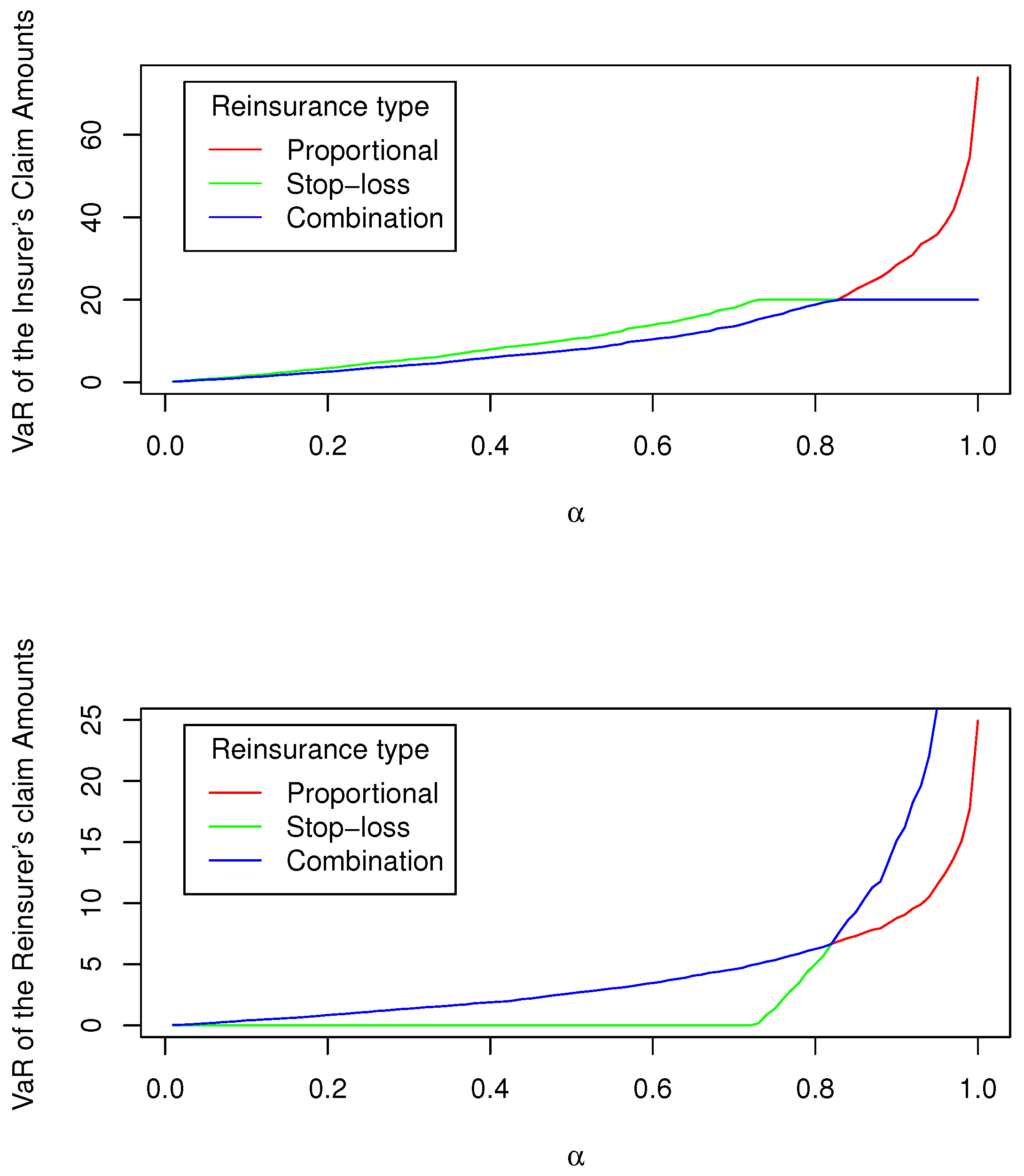
To compare the insurer’s claim amount and the reinsurer’s claim amount in the presence of proportional reinsurance, stop-loss reinsurance, and a combination of proportional and stop-loss reinsurance, we quantify them using a measure of tail risk, namely Value-at-Risk (VaR) (Barges et al. 2009). For the initial claim amount X, its VaR at a given confidence level α ( 0 , 1 ) is defined as the α -quantile of its distribution, i.e.,1
VaR α ( X ) = inf { x R : F X ( x ) α } ,
where F X ( x ) = 1 S X ( x ) = P ( X x ) is its distribution function. If this distribution function is continuous, VaR α ( X ) is a value of X satisfying the coverage probability equation F X ( VaR α ( X ) ) = P ( X VaR α ( X ) ) = α ; that is, VaR α ( X ) = F X 1 ( α ) . The resulting VaR for the insurer’s claim amount and the reinsurer’s claim amount is plotted in Figure 2.

2.2. Bivariate Models

Following Kang et al. (2021), we assume that both the insurer’s initial claim amount and the insurance premium are exponentially distributed, i.e., X E ( λ 1 ) and Y E ( λ 2 ) , with λ 1 , λ 2 > 0 . To capture their dependence, Sarmanov’s bivariate exponential distribution is considered. In addition, we define another choice of bivariate model, namely, the Farlie–Gumbel–Morgenstern (FGM) copula-based bivariate exponential distribution.
Definition 2.
Assume that both the insurer’s initial claim amount X and the insurance premium Y are exponentially distributed, i.e., X E ( λ 1 ) and Y E ( λ 2 ) , with λ 1 , λ 2 > 0 .
(a) 
Sarmanov’s Bivariate Exponential Distribution
As in Cossette et al. (2015) and Vernic (2016, 2017), the joint probability density function f X , Y ( x , y ) of X and Y under this distributional assumption is defined as follows:
f X , Y ( x , y ) = λ 1 λ 2 e ( λ 1 x + λ 2 y ) + θ λ 1 λ 2 ( λ 1 + 1 ) ( λ 2 + 1 ) i = 0 1 j = 0 1 ( 1 ) i + j ( λ 1 + i ) e ( λ 1 + i ) x ( λ 2 + j ) ( λ 2 + j ) y .
We assume that 0 < θ ( 1 + λ 1 ) ( 1 + λ 2 ) max ( λ 1 , λ 2 ) to ensure that their correlation coefficient ρ ( X , Y ) = θ λ 1 λ 2 ( 1 + λ 1 ) 2 ( 1 + λ 2 ) 2 is positive (Kang et al. 2021).
(b) 
The Bivariate Exponential Distribution with the Farlie–Gumbel–Morgenstern (FGM) Copula
The functional form of this copula is given by
C X , Y FGM ( F X ( x ) , F Y ( y ) ) = F X ( x ) F Y ( y ) [ 1 + θ ( 1 F X ( x ) ) ( 1 F Y ( y ) ) ] ,
with the corresponding copula density c X , Y FGM ( F X ( x ) , F Y ( y ) ) = 1 + θ ( 1 2 F X ( x ) ) ( 1 2 F Y ( y ) ) . The joint probability density function
f X , Y ( x , y ) = f X ( x ) f Y ( y ) c X , Y FGM ( F X ( x ) , F Y ( y ) )
of X and Y is determined by substituting F X ( x ) = 1 e λ 1 x , F Y ( y ) = 1 e λ 2 y , f X ( x ) = λ 1 e λ 1 x , and f Y ( y ) = λ 2 e λ 2 y . To make sure that they are positively correlated, the parameter θ of the FGM copula is assumed to belong to ( 0 , 1 ] (Barges et al. 2009; Kang et al. 2021).

3. Formulation of Reinsurance Optimization Problem

Under the combination of proportional and stop-loss reinsurance, the net cost (NC) of the insurer for a given policy is given by
NC = I R PSL ( X ; c , d ) + π ( I ( X R PSL ( X ; c , d ) ) ) Y .
We have some assumptions in Model (8) that are as follows. By assuming that both the initial claim amount X and the Bernoulli random variable I are independent, the insurer’s claim amount R PSL ( X ; c , d ) and I are also independent. Furthermore, I is independent of Y. In addition, Y and X are assumed to have a positive correlation.
We also assume that the reinsurance premium is calculated based on two fundamental premium principles: the expected value and the standard deviation. According to the expected value premium principle (EVPP) with the reinsurance loading factor β > 0 , the reinsurance premium is defined as
π EVPP ( I ( X R PSL ( X ; c , d ) ) ) = ( 1 + β ) E [ I ( X R PSL ( X ; c , d ) ) ] .
where E [ I ( X R PSL ( X ; c , d ) ) ] denotes the expectation of the claim amount paid by the reinsurer. Meanwhile, based on the standard deviation premium principle (SDPP), the reinsurance premium is defined as
π SDPP ( I ( X R PSL ( X ; c , d ) ) ) = E [ I ( X R PSL ( X ; c , d ) ) ] + β V [ I ( X R PSL ( X ; c , d ) ) ] ,
where V [ I ( X R PSL ( X ; c , d ) ) ] denotes the variance of the claim amount paid by the reinsurer.
As argued by Zhou et al. (2011) and Zheng and Cui (2014), the cedent of the claim amount means a reduction in profits. Therefore, there should be a reasonable restriction on the reinsurance premium for an insurer. Following their suggestions, we restrict the reinsurance premium as follows:
π ( I ( X R PSL ( X ; c , d ) ) ) P ,
where P denotes the maximum payment.
To measure the net cost of the insurer, we use the VaR risk measure defined in Equation (7). Accordingly, optimal reinsurance could be defined as a solution to the following optimization problem:
VaR α NC ; c * , d * = min c , d VaR α NC ; c , d
subject to
π ( I ( X R PSL ( X ; c , d ) ) ) P , ( c , d ) [ 0 , 1 ] × [ 0 , ) .

3.1. Sarmanov’s Bivariate Exponential Distribution

When the insurer’s claim amount and the insurance premium have Sarmanov’s bivariate exponential distribution, the reinsurance optimization determined by the VaR of the insurer’s net cost is provided in the following theorem.
Theorem 1.
Let the insurer’s claim amount X and the insurance premium Y have Sarmanov’s bivariate exponential distribution and 0 < α < 1 .
(a) 
If VaR α ( X ) d c , the optimal combination of proportional and stop-loss reinsurance is derived by minimizing
VaR α ( NC ; c , d ) = π ( I ( X c X ) ) + υ
subject to
( 1 c ) p λ 1 P 1 + β , ( c , d ) [ 0 , 1 ] × [ 0 , ) ,
where υ = VaR α ( c X I Y ) ,
α ( 1 p ) p δ 1 p = 1 λ 1 + λ 2 c c λ 2 + λ 1 e ( d c λ 1 + d λ 2 ) c λ 2 e υ c λ 1 λ 1 e ( d c λ 1 + d λ 2 υ λ 2 ) θ λ 1 λ 2 ( λ 1 + 1 ) ( λ 2 + 1 ) i = 0 1 j = 0 1 ( 1 ) i + j λ 1 + i + c ( λ 2 + j ) × c ( λ 2 + j ) e υ c ( λ 1 + i ) 1 ( λ 1 + i ) e υ ( λ 2 + j ) 1 e ( d c ( λ 1 + i ) + d ( λ 2 + j ) ) ,
and
δ 1 = λ 1 λ 1 + c λ 2 + θ λ 1 λ 2 ( λ 1 + 1 ) ( λ 2 + 1 ) i = 0 1 j = 0 1 ( 1 ) i + j λ 1 + i ( λ 1 + i ) + c ( λ 2 + j ) .
(b) 
If VaR α ( X ) > d c , the optimal combination of proportional and stop-loss reinsurance is derived by minimizing
VaR α ( NC ; c , d ) = π ( I ( X d ) ) + VaR α ( d I Y )
subject to
p 1 λ 1 d P 1 + β , ( c , d ) [ 0 , 1 ] × [ 0 , ) ,
where
VaR α ( d I Y ) = 1 λ 2 ln α ( 1 p ) p e d λ 2 p e d λ 2 + 1 .
The proof of the above theorem is provided in Appendix A.1.
Remark 1.
From Theorem 1a, we find that the objective function (10) is an implicit function in c, d, and υ. This is because Equation (11) is an implicit function in c, d, and υ. Therefore, this problem changes to the following optimization problem:
VaR α NC ; c * , d * , υ * = min c , d , υ [ π ( I ( X c X ) ) + υ ]
subject to
h 1 ( c , d , υ ) = 0 , ( 1 c ) p λ 1 P 1 + β , ( c , d ) [ 0 , 1 ] × [ 0 , ) ,
where
h 1 ( c , d , υ ) = α ( 1 p ) p δ 1 p + 1 λ 1 + λ 2 c c λ 2 + λ 1 e ( d c λ 1 + d λ 2 ) c λ 2 e υ c λ 1 λ 1 e ( d c λ 1 + d λ 2 υ λ 2 ) θ λ 1 λ 2 ( λ 1 + 1 ) ( λ 2 + 1 ) i = 0 1 j = 0 1 ( 1 ) i + j λ 1 + i + c ( λ 2 + j ) × c ( λ 2 + j ) e υ c ( λ 1 + i ) 1 ( λ 1 + i ) e υ ( λ 2 + j ) 1 e ( d c ( λ 1 + i ) + d ( λ 2 + j ) )
and
δ 1 = λ 1 λ 1 + c λ 2 + θ λ 1 λ 2 ( λ 1 + 1 ) ( λ 2 + 1 ) i = 0 1 j = 0 1 ( 1 ) i + j λ 1 + i ( λ 1 + i ) + c ( λ 2 + j ) .

3.2. Bivariate Exponential Distribution with the FGM Copula

When the bivariate exponential distribution for the insurer’s claim amount and the insurance premium is determined using the FGM copula, the reinsurance optimization problem formulated by the VaR of the insurer’s net cost is provided in the following theorem.
Theorem 2.
Let the insurer’s claim amount X and the insurance premium Y have a bivariate exponential distribution with the FGM copula and 0 < α < 1 .
(a) 
If VaR α ( X ) d c , the optimal combination of proportional and stop-loss reinsurance is derived by minimizing
VaR α ( NC ; c , d ) = π ( I ( X c X ) ) + υ
subject to
( 1 c ) p λ 1 P 1 + β , ( c , d ) [ 0 , 1 ] × [ 0 , ) ,
where υ = VaR α ( c X I Y ) ,
α ( 1 p ) p δ 2 p = ( 1 + θ ) ψ ( υ ; λ 1 , λ 2 ) + θ ψ ( υ ; 2 λ 1 , λ 2 ) + θ ψ ( υ ; λ 1 , 2 λ 2 ) θ ψ ( υ ; 2 λ 1 , 2 λ 2 ) ,
δ 2 = 1 c ( 1 + θ ) λ 2 λ 1 + c λ 2 + 2 c θ λ 1 + 2 c λ 2 + c θ λ 2 2 λ 1 + c λ 2 2 c θ λ 2 2 λ 1 + 2 c λ 2 ,
and
ψ ( υ ; λ 1 , λ 2 ) = λ 1 λ 2 λ 1 + c λ 2 1 λ 2 e υ λ 2 1 e ( d c λ 1 d λ 2 ) + c λ 1 e υ c λ 1 1 .
(b) 
If VaR α ( X ) > d c , the optimal combination of proportional and stop-loss reinsurance is derived by minimizing
VaR α ( NC ; c , d ) = π ( I ( X d ) ) + VaR α ( d I Y )
subject to
p 1 λ 1 d P 1 + β , ( c , d ) [ 0 , 1 ] × [ 0 , ) ,
where
VaR α ( d I Y ) = 1 λ 2 ln α ( 1 p ) p e d λ 2 p e d λ 2 + 1 .
The proof of the above theorem is provided in Appendix A.2.
Remark 2.
From Theorem 2a, we find that the objective function (14) is an implicit function in c, d, and υ. This is because Equation (15) is an implicit function in c, d, and υ. Therefore, this problem changes to the following optimization problem:
VaR α NC ; c * , d * , υ * = min c , d , υ [ π ( I ( X c X ) ) + υ ]
subject to
h 2 ( c , d , υ ) = 0 , ( 1 c ) p λ 1 P 1 + β , ( c , d ) [ 0 , 1 ] × [ 0 , ) ,
where
h 2 ( c , d , υ ) = α ( 1 p ) p δ 2 p ( 1 + θ ) ψ ( υ ; λ 1 , λ 2 ) + θ ψ ( υ ; 2 λ 1 , λ 2 ) + θ ψ ( υ ; λ 1 , 2 λ 2 ) θ ψ ( υ ; 2 λ 1 , 2 λ 2 ) ,
δ 2 = 1 c ( 1 + θ ) λ 2 λ 1 + c λ 2 + 2 c θ λ 1 + 2 c λ 2 + c θ λ 2 2 λ 1 + c λ 2 2 c θ λ 2 2 λ 1 + 2 c λ 2 ,
and
ψ ( υ ; λ 1 , λ 2 ) = λ 1 λ 2 λ 1 + c λ 2 1 λ 2 e υ λ 2 1 e ( d c λ 1 d λ 2 ) + c λ 1 e υ c λ 1 1 .

4. Numerical Examples

In this section, we provide some numerical examples in order to determine the optimal proportion c * and optimal retention limit d * . We illustrate the theoretical results numerically by using the NMinimize toolbox in Mathematica. NMinimize uses one of the four direct search algorithms (Nelder–Mead, differential evolution, simulated annealing, and random search) and then fine-tunes the solution by using a combination of the Karush–Kuhn–Tucker (KKT) solution, the interior point, and a penalty method. Thus, NMinimize always attempts to find a global minimum subject to the constraints (see Champion and Strzebonski 2008). Referring to Kang et al. (2021) and He et al. (2022), we set the basic model parameters given in Table 1, where the insurer’s initial claim amount X and the insurance premium Y follow an exponential distribution with E [ X ] = 15 and E [ Y ] = 10 , respectively, and I follows a Bernoulli distribution with parameter p = 0.2 , 0.5 , 0.8 . Their dependence is modeled using Sarmanov’s bivariate model (Case 1) and the FGM copula (Case 2) with dependence parameter θ = 0 , 0.2 , 0.5 , where θ = 0 indicates that they are uncorrelated. The reinsurance premium is assumed to be charged by the expected value premium principle (EVPP) and standard deviation premium principle (SDPP).
Using the NMinimize toolbox in Mathematica, we derive c * , d * , υ * , and the corresponding VaR α ( NC ; c * , d * , υ * ) provided in Table 2, Table 3, Table 4 and Table 5 for various values of the dependence parameter θ , the probability of claim occurrence p, and the confidence level α for Case 1 and Case 2 under the EVPP and SDPP. Based on the four tables, we see that if there is no correlation between the claim amount and the insurance premium (i.e., θ = 0 ) for each case and reinsurance premium principle, then the optimal VaR of the insurer’s net cost VaR α ( NC ; c * , d * , υ * ) always increases with the increase in the confidence level α .
In this section, we also conduct some numerical simulations to illustrate the effects of the confidence level α , the dependence parameter θ , and the probability of claim occurrence p on the optimal VaR of the insurer’s net cost VaR α ( NC ; c * , d * , υ * ) for each case and reinsurance premium principle. The results are depicted in Figure 3, Figure 4, Figure 5 and Figure 6.
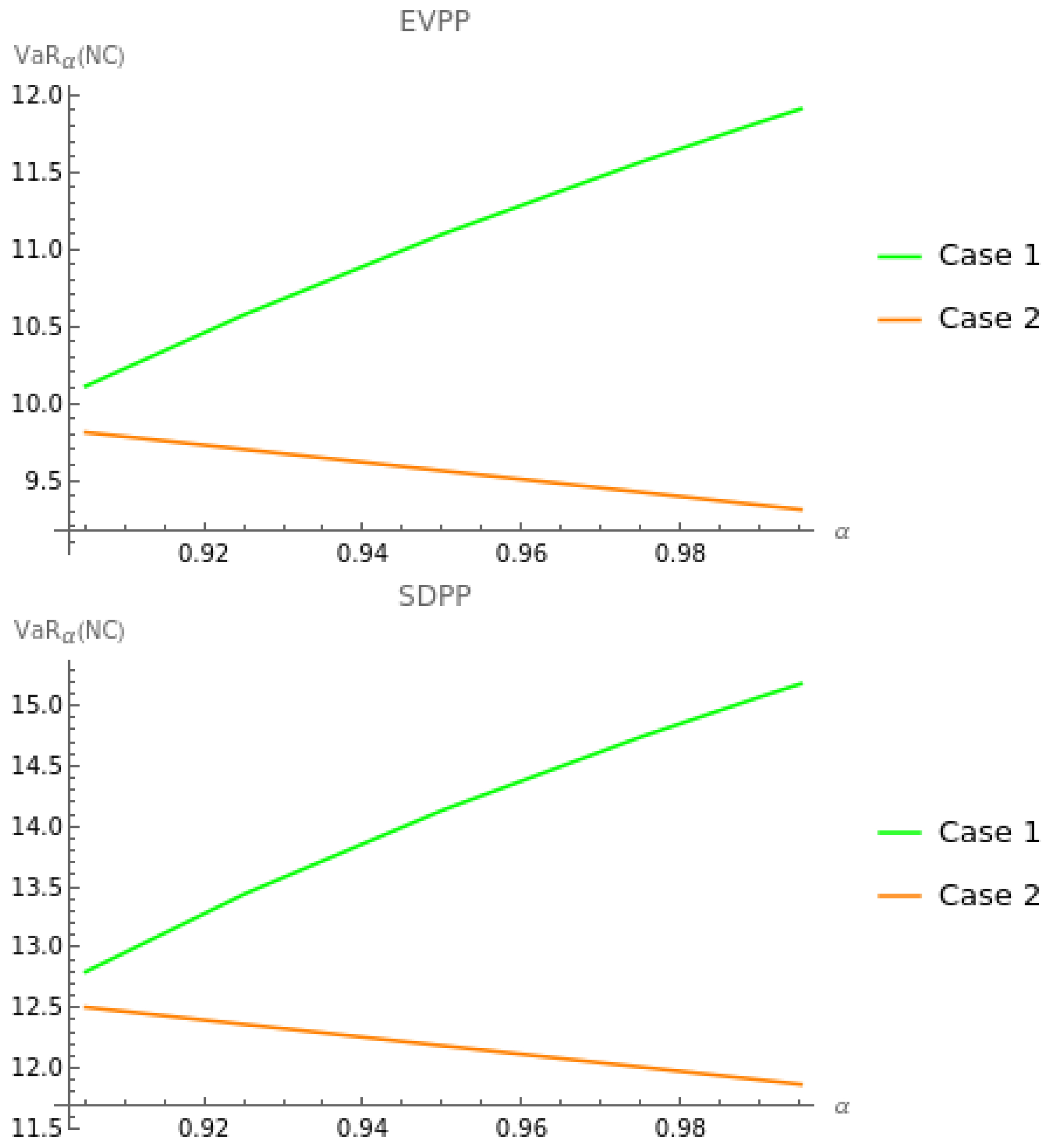
Figure 3 shows the effects of the confidence level α on the optimal VaR of the insurer’s net cost VaR α ( NC ; c * , d * , υ * ) for each case and reinsurance premium principle. For Case 1, we observe that VaR α ( NC ; c * , d * , υ * ) increases with the increase in α . This means that the larger the value of α is, the more aggressive the insurer is about the risks. Meanwhile, for Case 2, we find that VaR α ( NC ; c * , d * , υ * ) decreases with the increase in α . This indicates that the FGM copula makes VaR α ( NC ; c * , d * , υ * ) become smaller when the insurer is more aggressive about the risks.
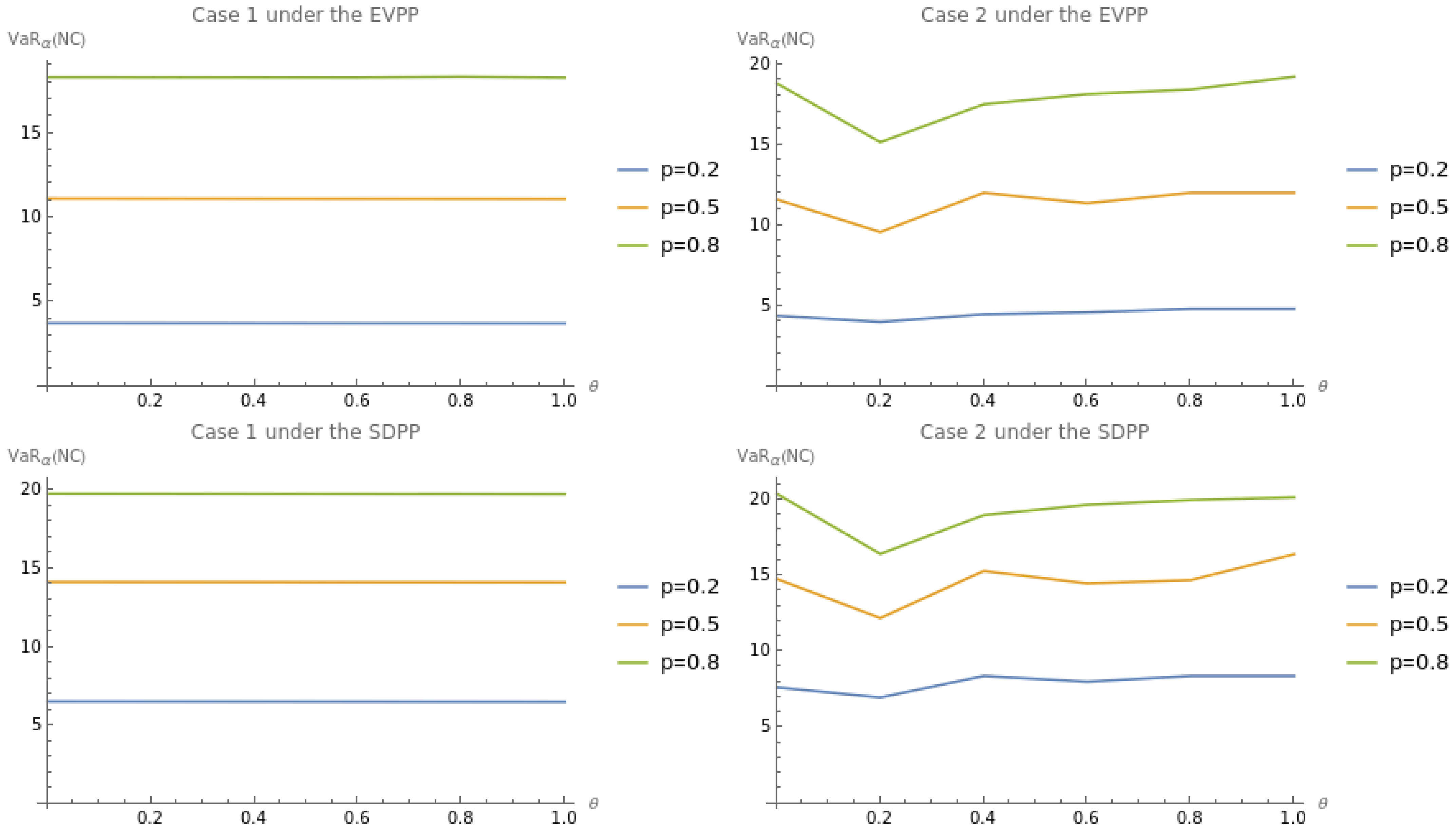
Figure 4 demonstrates the effects of both the dependence parameter θ and the probability of claim occurrence p on the optimal VaR of the insurer’s net cost VaR α ( NC ; c * , d * , υ * ) for each case and reinsurance premium principle. For Case 1, we see that VaR α ( NC ; c * , d * , υ * ) decreases with the increase in both θ and p. Meanwhile, for Case 2, VaR α ( NC ; c * , d * , υ * ) increases and decreases with the increase in both θ and p. Furthermore, VaR α ( NC ; c * , d * , υ * ) derived under the SDPP is found to be larger than that determined under the EVPP.
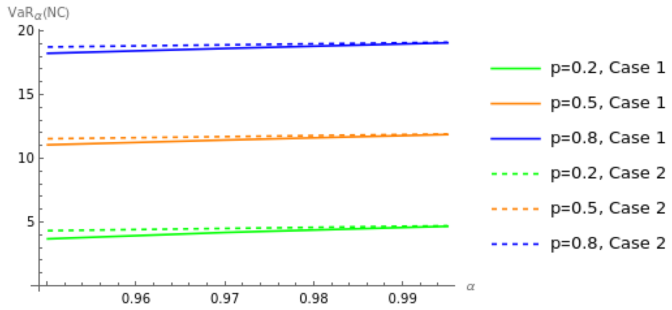
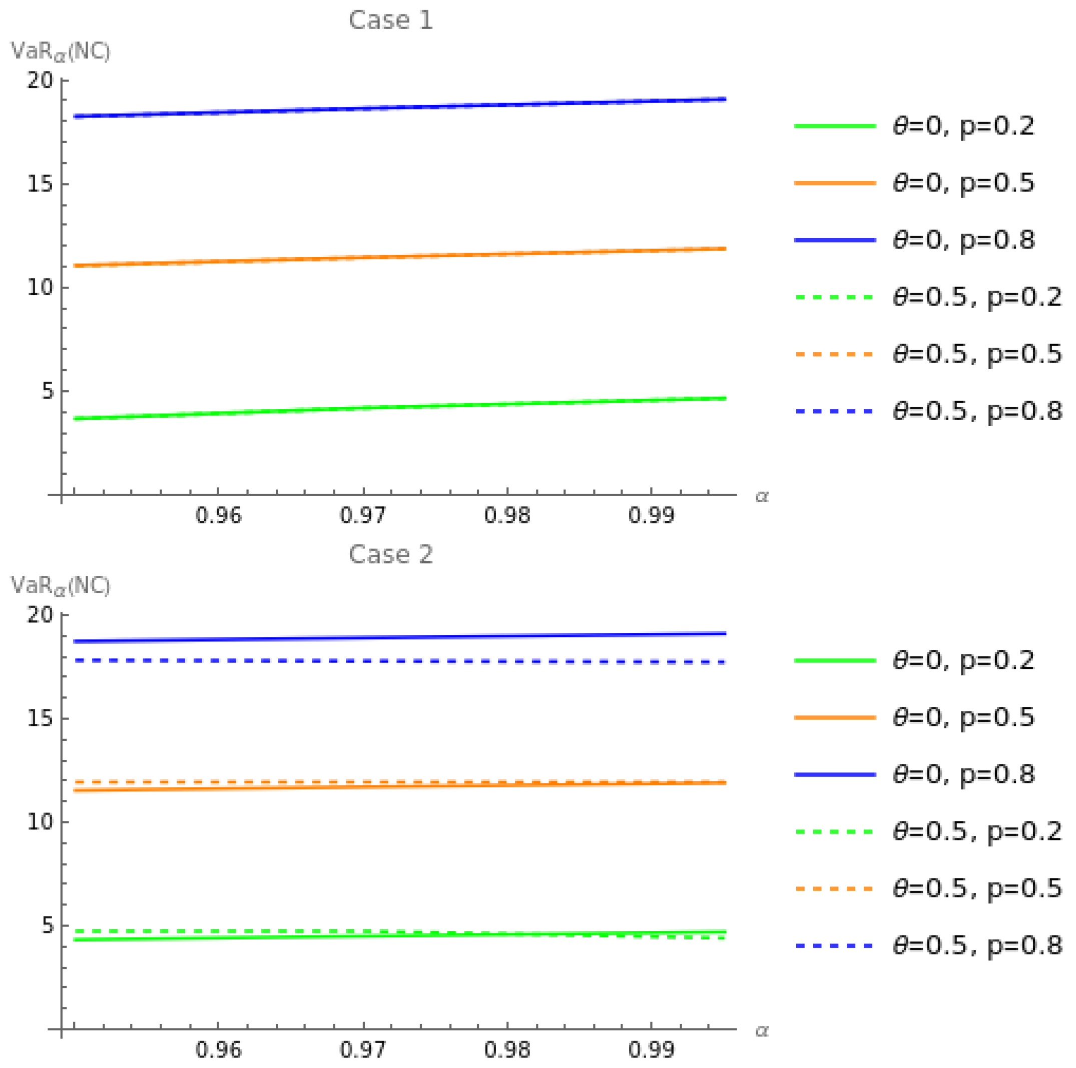
Figure 5 illustrates the effects of θ = 0 (no correlation between X and Y) on the optimal VaR of the insurer’s net cost VaR α ( NC ; c * , d * , υ * ) for Case 1 (Sarmanov’s bivariate exponential distribution) and Case 2 (bivariate exponential distribution with the FGM copula) under the EVPP. We find that VaR α ( NC ; c * , d * , υ * ) for Case 1 is smaller than that for Case 2. This is because of the effect of the FGM copula.
In Figure 6, we analyze the effects of θ = 0 and θ = 0.5 on the optimal VaR of the insurer’s net cost VaR α ( NC ; c * , d * , υ * ) for the two cases under the EVPP when p = 0.2 , 0.5 , 0.8 and find three aspects. First, no matter whether the positive correlation between the claim amount X and the insurance premium Y exists (i.e., θ = 0.5 ) or does not exist (i.e., θ = 0 ), VaR α ( NC ; c * , d * , υ * ) increases with the increase in the probability of claim occurrence p. Second, we find for Case 1 that VaR α ( NC ; c * , d * , υ * ) derived when θ = 0 is approximately equal to that determined when θ = 0.5 . Third, in Case 2, when the positive correlation exists (i.e., θ = 0.5 ), and the probability of claim occurrence is equal to p = 0.8 , the insurer considerably reduces the magnitude of the optimal VaR of their net cost.

5. Conclusions

Our study focuses on modeling the optimal combination of proportional and stop-loss reinsurance with the dependent claim and stochastic insurance premium. To capture their dependence structure, we use two bivariate models: Sarmanov’s bivariate exponential distribution (Case 1) and the FGM copula-based bivariate exponential distribution (Case 2). With the reinsurance premium determined by the expected value premium principle (EVPP) and standard deviation premium principle (SDPP), we use the minimization of the Value-at-Risk (VaR) of the insurer’s net cost and a constrained reinsurance premium as optimization criteria. We first derive the insurer’s net cost, which is an implicit function, making this study become challenging. Using the NMinimize toolbox in Mathematica, we provide numerical examples in order to determine the optimal proportion, the optimal retention limit, and the optimal VaR of the insurer’s net cost. We also analyze the effects of the dependence parameter, the probability of claim occurrence, and the confidence level on the optimal VaR of the insurer’s net cost.
Our numerical study provides the following results. (1) The correlation between the claim amount and the insurance premium influences the optimal VaR of the insurer’s net cost. Under each reinsurance premium principle, the optimal VaR of the insurer’s net cost decreases with the increase in the dependence parameter of Sarmanov’s bivariate. In contrast, it decreases and increases with the increase in the dependence parameter of the FGM copula. (2) The optimal VaR of the insurer’s net cost for Case 1 (Sarmanov’s bivariate exponential distribution) is smaller than that for Case 2 (bivariate exponential distribution with the FGM copula) when no positive correlation exists. However, if a positive correlation exists, the former is not always smaller than the latter. (3) The optimal VaR of the insurer’s net cost derived under the SDPP is larger than that determined under the EVPP. This is because of the effect of the variance of the claim amount paid by the reinsurer under the SDPP. (4) The effects of the dependence parameter and the confidence level on the optimal VaR of the insurer’s net cost for Case 1 are different from that for Case 2, while the effects of the probability of claim occurrence are always the same for both cases; see Figure 3 and Figure 4. More specifically, the optimal VaR of the insurer’s net cost increases with the increase in the probability of claim occurrence.
Our study focuses on one line of business. In future research, it would be interesting and challenging to extend our model to two or more lines of business. Furthermore, we may also use other bivariate models to capture the dependence structure between the claim amount and the insurance premium; see, e.g., Vidmar (2018) and Kang et al. (2021).

Author Contributions

Conceptualization, S.S., A.H. and K.S.; methodology, S.S. and K.S.; validation, A.H.; formal analysis, S.S. and K.S.; resources, I.M.; data curation, S.S.; writing—original draft preparation, S.S., A.H. and K.S.; writing—review and editing, S.S. and K.S.; supervision, I.M. and K.S.; project administration, I.M.; funding acquisition, K.S. All authors have read and agreed to the published version of the manuscript.

Funding

This work was funded by the Institut Teknologi Bandung (ITB)/Kemendikbudristek, Indonesia, under the grant of PDD 2021.

Institutional Review Board Statement

Not applicable.

Informed Consent Statement

Not applicable.

Data Availability Statement

No new data were created or analyzed in this study. Data sharing is not applicable to this article.

Acknowledgments

The authors are grateful to the academic editor’s and anonymous reviewers’ careful reading and valuable comments that greatly improved the quality of this paper. This work is part of the dissertation research of the first author (S.S.). She would like to thank the Universitas Indonesia (UI), Indonesia, which financially supported her doctoral study at the Institut Teknologi Bandung (ITB), Indonesia.

Conflicts of Interest

The authors declare no conflict of interest. The funders had no role in the design of the study; in the collection, analyses, or interpretation of data; in the writing of the manuscript; or in the decision to publish the results.

Appendix A

Appendix A.1. Proof of Theorem 1

Proof. 
Theorem 1a.
Define C = c X I Y and L = c X Y . In the event that I = 1 and c X Y , the loss is zero, i.e., C = 0 . Consider that
P ( c X Y ) = P X Y c = 0 0 y c f X , Y ( x , y ) d x d y = 0 0 y c λ 1 λ 2 e ( λ 1 x + λ 2 y ) + θ λ 1 λ 2 ( λ 1 + 1 ) ( λ 2 + 1 ) i = 0 1 j = 0 1 ( 1 ) i + j ( λ 1 + i ) e ( λ 1 + i ) x ( λ 2 + j ) e ( λ 2 + j ) y d x d y = λ 1 λ 1 + c λ 2 + θ λ 1 λ 2 ( λ 1 + 1 ) ( λ 2 + 1 ) i = 0 1 j = 0 1 ( 1 ) i + j λ 1 + i ( λ 1 + i ) + c ( λ 2 + j )
we denote by δ 1 . If I = 1 and c X Y , the loss exceeds zero, i.e., C > 0 . Next, we obtain
f L ( l ) = l c d c f X , Y ( x , c x l ) d x = l c d c λ 1 λ 2 e ( λ 1 x + λ 2 ( c x l ) ) + θ λ 1 λ 2 ( λ 1 + 1 ) ( λ 2 + 1 ) i = 0 1 j = 0 1 ( 1 ) i + j ( λ 1 + i ) e ( λ 1 + i ) x ( λ 2 + j ) e ( λ 2 + j ) ( c x l ) d x = λ 1 λ 2 λ 1 + λ 2 c e λ 1 c l e ( d c λ 1 + d λ 2 λ 2 l ) θ λ 1 λ 2 ( λ 1 + 1 ) ( λ 2 + 1 ) i = 0 1 j = 0 1 ( λ 1 + i ) ( λ 2 + j ) λ 1 + i + c ( λ 2 + j ) e ( d c ( λ 1 + i ) + d ( λ 2 + j ) ( λ 2 + j ) l ) e ( λ 1 + i c ) l .
By Equation (8), the VaR of the net loss of the insurer is VaR α ( NC ; c , d ) = π ( X I c X I ) + VaR α ( C ) , where the VaR α ( C ) satisfies
α = P ( C VaR α ( C ) ) = P ( I = 0 ) + P ( I = 1 ) P ( c X Y ) + P ( I = 1 ) P ( 0 < L VaR α ( C ) ) = ( 1 p ) + p δ 1 + p P ( 0 < L VaR α ( C ) ) .
Thus,
α ( 1 p ) p δ i p = P ( 0 < L VaR α ( C ) ) = 0 VaR α ( C ) λ 1 λ 2 λ 1 + c λ 2 e λ 1 c l e ( d c λ 1 + d λ 2 λ 2 l ) θ λ 1 λ 2 ( λ 1 + 1 ) ( λ 2 + 1 ) i = 0 1 j = 0 1 ( 1 ) i + j ( λ 1 + i ) ( λ 2 + j ) λ 1 + i + c ( λ 2 + j ) × e ( d c ( λ 1 + i ) + d ( λ 2 + j ) ( λ 2 + j ) l ) e ( λ 1 + i c ) l d l .
For the sake of simplicity, let VaR α ( C ) = υ . Therefore, the above equation can be written as
α ( 1 p ) p δ 1 p = 1 λ 1 + c λ 2 c λ 2 + λ 1 e ( d c λ 1 + d λ 2 ) c λ 2 e υ c λ 1 λ 1 e ( d c λ 1 + d λ 2 υ λ 2 ) θ λ 1 λ 2 ( λ 1 + 1 ) ( λ 2 + 1 ) i = 0 1 j = 0 1 ( 1 ) i + j λ 1 + i + c ( λ 2 + j ) × c ( λ 2 + j ) e υ c ( λ 1 + i ) 1 ( λ 1 + i ) e υ ( λ 2 + j ) 1 e ( d c ( λ 1 + i ) + d ( λ 2 + j ) ) .
Proof. 
Theorem 1b.
Define C = d I Y and L = d Y . In the event that I = 1 and d Y , the loss is zero, i.e., C = 0 . Consider that
P ( d Y ) = P Y d = S Y ( d ) = e d λ 2 .
If I = 1 and d Y , the loss exceeds zero, i.e., C > 0 . Next, we obtain
P L l = P d Y l = P Y > d l F L ( l ) = e λ 2 ( d l ) .
Then, f L ( l ) = λ 2 e λ 2 ( d l ) . By Equation (8), the VaR of the net loss of the insurer is VaR α ( NC ; c , d ) = π ( I ( X d ) ) + VaR α ( C ) , where VaR α ( C ) satisfies
α = P ( C VaR α ( C ) ) = P ( I = 0 ) + P ( I = 1 ) P ( d Y ) + P ( I = 1 ) P ( 0 < L VaR α ( C ) ) = ( 1 p ) + p e d λ 2 + p P ( 0 < L VaR α ( C ) ) .
Thus,
α ( 1 p ) p e d λ 2 p = P ( 0 < L VaR α ( C ) ) = 0 VaR α ( C ) λ 2 e λ 2 ( d l ) d l = e d λ 2 e λ 2 VaR α ( C ) 1 .
Therefore, the above equation can be written as
VaR α ( C ) = 1 λ 2 ln α ( 1 p ) p e d λ 2 p e d λ 2 + 1 .

Appendix A.2. Proof of Theorem 2

Proof. 
Theorem 2a.
Define C = c X I Y and L = c X Y . In the event that I = 1 and c X Y , the loss is zero, i.e., C = 0 . Consider that
P ( c X Y ) = P X Y c = 0 0 y c f X , Y ( x , y ) d x d y = 0 0 y c ( 1 + θ ) λ 1 λ 2 e ( λ 1 x + λ 2 y ) 2 θ λ 1 λ 2 e ( λ 1 x + 2 λ 2 y ) 2 θ λ 1 λ 2 e ( 2 λ 1 x + λ 2 y ) + 4 θ λ 1 λ 2 e ( 2 λ 1 x + 2 λ 2 y ) d x d y = 1 c ( 1 + θ ) λ 2 λ 1 + c λ 2 + 2 c θ λ 1 + 2 c λ 2 + c θ λ 2 2 λ 1 + c λ 2 2 c θ λ 2 2 λ 1 + 2 c λ 2 ,
which we denote by δ 2 . If I = 1 and c X Y , the loss exceeds zero, i.e., C > 0 . Next, we obtain
f L ( l ) = l c d c f X , Y ( x , c x l ) d x = l c d c ( 1 + θ ) λ 1 λ 2 e ( λ 1 x + λ 2 ( c x l ) ) 2 θ λ 1 λ 2 e ( λ 1 x + 2 λ 2 ( c x l ) ) 2 θ λ 1 λ 2 e ( 2 λ 1 x + λ 2 ( c x l ) ) + 4 θ λ 1 λ 2 e ( 2 λ 1 x + 2 λ 2 ( c x l ) ) d x = ( 1 + θ ) λ 1 λ 2 λ 1 + c λ 2 e ( d c λ 1 + d λ 2 l λ 2 ) e l c λ 1 + 2 θ λ 1 λ 2 2 λ 1 + λ 2 c e ( 2 d c λ 1 + d λ 2 l λ 2 ) e 2 l c λ 1 + 2 θ λ 1 λ 2 λ 1 + 2 c λ 2 e ( d c λ 1 + 2 d λ 2 2 l λ 2 ) e l c λ 1 2 θ λ 1 λ 2 λ 1 + λ 2 c e ( 2 d c λ 1 + 2 d λ 2 2 l λ 2 ) e 2 l c λ 1 .
By Equation (8), the VaR of the insurer’s net loss is VaR α ( NC ; c , d ) = π ( X I c X I ) + VaR α ( C ) , where VaR α ( C ) satisfies
α = P ( C VaR α ( C ) ) = P ( I = 0 ) + P ( I = 1 ) P ( c X Y ) + P ( I = 1 ) P ( 0 < L VaR α ( C ) ) = ( 1 p ) + p δ 2 + p P ( 0 < L VaR α ( C ) ) .
Therefore,
α ( 1 p ) p δ 2 p = P ( 0 < L VaR α ( C ) ) = 0 VaR α ( C ) ( 1 + θ ) λ 1 λ 2 λ 1 + c λ 2 e ( d c λ 1 + d λ 2 l λ 2 ) e l c λ 1 + 2 θ λ 1 λ 2 2 λ 1 + c λ 2 e ( 2 d c λ 1 + d λ 2 l λ 2 ) e 2 l c λ 1 + 2 θ λ 1 λ 2 λ 1 + 2 c λ 2 e ( d c λ 1 + 2 d λ 2 2 l λ 2 ) e l c λ 1 2 θ λ 1 λ 2 λ 1 + c λ 2 e ( 2 d c λ 1 + 2 d λ 2 2 l λ 2 ) e 2 l c λ 1 d l .
For the sake of simplicity, let VaR α ( C ) = υ . Thus, the above equation can be expressed as
α ( 1 p ) p δ 2 p = ( 1 + θ ) λ 1 λ 2 λ 1 + c λ 2 1 λ 2 e ( d c λ 1 + d λ 2 l λ 2 ) + c λ 1 e l c λ 1 + 2 θ λ 1 λ 2 2 λ 1 + c λ 2 1 λ 2 e ( 2 d c λ 1 + d λ 2 l λ 2 ) + c 2 λ 1 e 2 l c λ 1 + 2 θ λ 1 λ 2 λ 1 + 2 c λ 2 1 2 λ 2 e ( d c λ 1 + 2 d λ 2 2 l λ 2 ) + c λ 1 e l c λ 1 2 θ λ 1 λ 2 λ 1 + c λ 2 1 2 λ 2 e ( 2 d c λ 1 + 2 d λ 2 2 l λ 2 ) + c 2 λ 1 e 2 l c λ 1
or can be written as
α ( 1 p ) p δ 2 p = ( 1 + θ ) ψ ( υ ; λ 1 , λ 2 ) + θ ψ ( υ ; 2 λ 1 , λ 2 ) + θ ψ ( υ ; λ 1 , 2 λ 2 ) θ ψ ( υ ; 2 λ 1 , 2 λ 2 ) ,
where
ψ ( υ ; λ 1 , λ 2 ) = λ 1 λ 2 λ 1 + c λ 2 1 λ 2 e υ λ 2 1 e ( d c λ 1 d λ 2 ) + c λ 1 e υ c λ 1 1 .

Note

1
When X is a profit-and-loss (P&L) random variable denoting, e.g., a financial position or a financial asset return, the VaR of X at a given significance level α is defined as the negative of its lower α -quantile, i.e., VaR α ( X ) = inf { x R : F X ( x ) α } ; see Artzner et al. (1999).

References

  1. Artzner, Philippe, Freddy Delbaen, Jean-Marc Eber, and David Heath. 1999. Coherent Measures of Risk. Mathematical Finance 9: 203–28. [Google Scholar] [CrossRef]
  2. Bao, Zhen-hua. 2006. The Expected Discounted Penalty at Ruin in the Risk Process with Random Income. Applied Mathematics and Computation 179: 559–66. [Google Scholar] [CrossRef]
  3. Bao, Zhen-hua, and Zhong-xing Ye. 2007. The Gerber–Shiu Discounted Penalty Function in the Delayed Renewal Risk Process with Random Income. Applied Mathematics and Computation 184: 857–63. [Google Scholar] [CrossRef]
  4. Bargès, Mathieu, Hélène Cossette, and Étienne Marceau. 2009. TVaR-Based Capital Allocation with Copulas. Insurance: Mathematics and Economics 45: 348–61. [Google Scholar] [CrossRef]
  5. Borch, Karl. 1960. The Safety Loading of Reinsurance Premiums. Scandinavian Actuarial Journal 1960: 163–84. [Google Scholar] [CrossRef]
  6. Brachetta, Matteo, and Claudia Ceci. 2019. Optimal Excess-of-Loss Reinsurance for Stochastic Factor Risk Models. Risks 7: 48. [Google Scholar] [CrossRef]
  7. Cai, Jun, Christiane Lemieux, and Fangda Liu. 2016. Optimal Reinsurance from the Perspectives of Both an Insurer and a Reinsurer. ASTIN Bulletin: The Journal of the IAA 46: 815–49. [Google Scholar] [CrossRef]
  8. Cai, Jun, and Ken S. Tan. 2007. Optimal Retention for a Stop-Loss Reinsurance under the VaR and CTE Risk Measure. ASTIN Bulletin: The Journal of the IAA 37: 93–112. [Google Scholar] [CrossRef]
  9. Cai, Jun, Ken S. Tan, Chengguo Weng, and Yi Zhang. 2008. Optimal Reinsurance under VaR and CTE Risk Measures. Insurance: Mathematics and Economics 43: 185–96. [Google Scholar] [CrossRef]
  10. Champion, Brett, and Adam Strzebonski. 2008. Wolfram Mathematica Tutorial Collection: Constrained Optimization. Wolfram Library Archive. Available online: https://library.wolfram.com/infocenter/Books/8506 (accessed on 14 July 2022).
  11. Chen, Yanhong, and Yijun Hu. 2021. Optimal Reinsurance from the Perspectives of Both Insurers and Reinsurers under the VaR Risk Measure and Vajda Condition. Communications in Statistics: Theory and Methods 50: 3677–94. [Google Scholar] [CrossRef]
  12. Chi, Yichun. 2012. Optimal Reinsurance under Variance Related Premium Principles. Insurance: Mathematics and Economics 51: 310–21. [Google Scholar] [CrossRef]
  13. Chi, Yichun, and Ken S. Tan. 2011. Optimal Reinsurance under VaR and CVaR Risk Measures: A Simplified Approach. ASTIN Bulletin: The Journal of the IAA 41: 487–509. [Google Scholar]
  14. Cossette, Hélène, Etienne Marceau, and Samuel Perreault. 2015. On Two Families of Bivariate Distributions with Exponential Marginals: Aggregation and Capital Allocation. Insurance: Mathematics and Economics 64: 214–24. [Google Scholar] [CrossRef]
  15. Gajek, Lesław, and Dariusz Zagrodny. 2000. Insurer’s Optimal Reinsurance Strategies. Insurance: Mathematics and Economics 27: 105–12. [Google Scholar] [CrossRef]
  16. He, Xinya, Ailing Gu, and Haixiang Yao. 2022. Stochastic Differential Reinsurance and Investment Games with Delay under VaR Constraints. Communications in Statistics: Theory and Methods, in press. [Google Scholar]
  17. Kahn, Paul M. 1961. Some Remarks on a Recent Paper by Borch. ASTIN Bulletin: The Journal of the IAA 1: 265–72. [Google Scholar] [CrossRef]
  18. Kaluszka, Marek. 2004. Mean-Variance Optimal Reinsurance Arrangements. Scandinavian Actuarial Journal 2004: 28–41. [Google Scholar] [CrossRef]
  19. Kang, Yao, Dehui Wang, and Jianhua Cheng. 2021. Risk Models Based on Copulas for Premiums and Claim Sizes. Communications in Statistics: Theory and Methods 50: 2250–69. [Google Scholar] [CrossRef]
  20. Karageyik, Başak B., and Şule Şahin. 2017. Determination of the Optimal Retention Level Based on Different Measures. Journal of Risk and Financial Management 10: 4. [Google Scholar] [CrossRef]
  21. Khare, Shree, and Keven Roy. 2021. Quantifying the Role of Occurrence Losses in Catastrophe Excess of Loss Reinsurance Pricing. Risks 9: 52. [Google Scholar] [CrossRef]
  22. Liang, Zhibin, and Kam C. Yuen. 2016. Optimal Dynamic Reinsurance with Dependent Risks: Variance Premium Principle. Scandinavian Actuarial Journal 2016: 18–36. [Google Scholar] [CrossRef]
  23. Ohlin, Jan. 1969. On a Class of Measures of Dispersion with Application to Optimal Reinsurance. ASTIN Bulletin: The Journal of the IAA 5: 249–66. [Google Scholar] [CrossRef] [Green Version]
  24. Sari, Suci F., and Khreshna I. A. Syuhada. 2022. Tail Risk Measures-Based Optimal Reinsurance Model for Quota-Share Reinsurance. AIP Conference Proceedings 2471: 020010. [Google Scholar]
  25. Syuhada, Khreshna, Arief Hakim, and Suci Sari. 2021. The Combined Stop-Loss and Quota-Share Reinsurance: Conditional Tail Expectation-Based Optimization from the Joint Perspective of Insurer and Reinsurer. Risks 9: 125. [Google Scholar] [CrossRef]
  26. Tan, Ken S., Chengguo Weng, and Yi Zhang. 2009. VaR and CTE Criteria for Optimal Quota-Share and Stop-Loss Reinsurance. North American Actuarial Journal 13: 459–82. [Google Scholar] [CrossRef]
  27. Tan, Tao, Tao Chen, Lijun Wu, Yuhong Sheng, and Yijun Hu. 2020. VaR and CTE Based Optimal Reinsurance from a Reinsurer’s Perspective. Acta Mathematica Scientia 40: 1915–27. [Google Scholar] [CrossRef]
  28. Temnov, G. 2004. Risk Process with Random Income. Journal of Mathematical Sciences 123: 3780–94. [Google Scholar] [CrossRef]
  29. Vernic, Raluca. 2016. On the Distribution of a Sum of Sarmanov Distributed Random Variables. Journal of Theoretical Probability 29: 118–42. [Google Scholar] [CrossRef]
  30. Vernic, Raluca. 2017. Capital Allocation for Sarmanov’s Class of Distributions. Methodology and Computing in Applied Probability 19: 311–30. [Google Scholar] [CrossRef]
  31. Vidmar, Matija. 2018. Ruin under Stochastic Dependence between Premium and Claim Arrivals. Scandinavian Actuarial Journal 2018: 505–13. [Google Scholar] [CrossRef]
  32. Zhang, Nan, Zhuo Jin, Linyi Qian, and Rongming Wang. 2018. Optimal Quota-Share Reinsurance Based on the Mutual Benefit of Insurer and Reinsurer. Journal of Computational and Applied Mathematics 342: 337–51. [Google Scholar] [CrossRef]
  33. Zheng, Yanting, and Wei Cui. 2014. Optimal Reinsurance with Premium Constraint under Distortion Risk Measures. Insurance: Mathematics and Economics 59: 109–20. [Google Scholar] [CrossRef]
  34. Zhou, Ming, Hongbin Dong, and Jingfeng Xu. 2011. Optimal Combinational of Quota-Share and Stop-Loss Reinsurance Contracts under VaR and CTE with a Constrained Reinsurance Premium. Journal of Systems Science and Complexity 24: 156–66. [Google Scholar] [CrossRef]
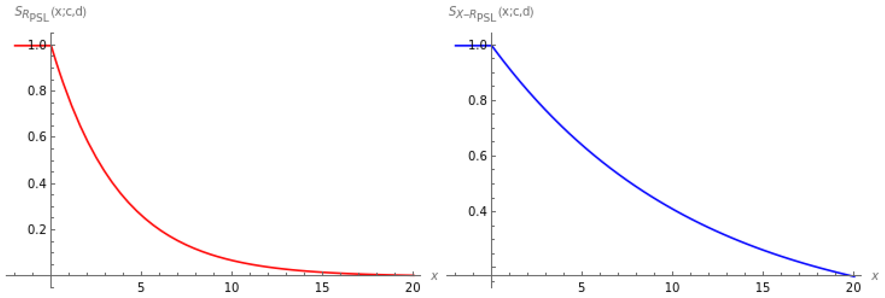
Figure 1. Graphical representation of the survival functions S R PSL ( X ) ( x ; c , d ) and S X R PSL ( X ) ( x ; c , d ) under a combination of proportional and stop-loss reinsurance with c = 75 % and d = 20 when the initial claim amount X follows an exponential distribution ( λ = 1 / 15 ).
Jrfm 16 00095 g001
Figure 2. Graphical representation of the insurer’s claim amount and the reinsurer’s claim amount measured using VaR at the α confidence level under proportional reinsurance with c = 75 % (the red curve), stop-loss reinsurance with d = 20 (the green curve), and a combination of proportional and stop-loss reinsurance with c = 75 % and d = 20 (the blue curve) when the initial claim amount X follows an exponential distribution ( λ = 1 / 15 ).
Jrfm 16 00095 g002
Figure 3. Effects of α on VaR α ( NC ; c * , d * , υ * ) for Case 1 and Case 2 under the EVPP and SDPP when θ = 0.2 and p = 0.5 are fixed.
Jrfm 16 00095 g003
Figure 4. Effects of θ and p on VaR α ( NC ; c * , d * , υ * ) for Case 1 and Case 2 under the EVPP and SDPP when α = 0.950 is fixed.
Jrfm 16 00095 g004
Figure 5. Effects of θ = 0 (no correlation between X and Y) on VaR α ( NC ; c * , d * , υ * ) under the EVPP when p = 0.2 , 0.5 , 0.8 .
Jrfm 16 00095 g005
Figure 6. Effects of θ = 0 versus θ = 0.5 on VaR α ( NC ; c * , d * , υ * ) under the EVPP when p = 0.2 , 0.5 , 0.8 .
Jrfm 16 00095 g006
Table 1. Basic model parameters.
λ 1 λ 2 β P θ p α
Value 11/151/100.66000.20.950
Value 2 0.20.50.970
Value 3 0.50.80.995
Table 2. Optimal combination of proportional and stop-loss reinsurance and the resulting VaR α ( NC ; c * , d * , υ * ) for Case 1 under the EVPP.
θ p α c * d * υ * VaR α ( NC ; c * , d * , υ * )
00.20.9500.222274.5959.763 × 10 9 3.733
0.9700.118168.9790.0004.235
0.9950.0172.629 × 10 7 9.131 × 10 11 4.718
0.50.9500.0743.347 × 10 15 0.00011.111
0.9700.0434.485 × 10 16 0.00011.489
0.9950.0071.797 × 10 18 0.00011.919
0.80.9500.066254.8160.36918.295
0.9700.0372.995 × 10 6 0.18318.677
0.9950.0061.439 × 10 6 0.02419.117
0.20.20.9500.2230.0000.0003.731
0.9700.118262.6980.0004.233
0.9950.017124.3230.0004.717
0.50.9500.0741.215 × 10 7 1.781 × 10 12 11.107
0.9700.0433.504 × 10 16 0.00011.486
0.9950.0071.145 × 10 17 0.00011.918
0.80.9500.0671.111 × 10 6 0.36918.290
0.9700.0373.528 × 10 6 0.18418.674
0.9950.0065.633 × 10 6 0.02519.116
0.50.20.9500.224336.4206.758 × 10 9 3.727
0.9700.119185.5750.0004.230
0.9950.01895.8370.0004.716
0.50.9500.0757.452 × 10 6 3.298 × 10 8 11.100
0.9700.0433.579 × 10 6 9.062 × 10 12 11.481
0.9950.007128.7014.854 × 10 6 11.917
0.80.9500.0671.108 × 10 6 0.36818.283
0.9700.0271.057 × 10 17 0.00018.692
0.9950.0061.146 × 10 7 0.02619.114
Table 3. Optimal combination of proportional and stop-loss reinsurance and the resulting VaR α ( NC ; c * , d * , υ * ) for Case 1 under the SDPP.
θ p α c * d * υ * VaR α ( NC ; c * , d * , υ * )
00.20.9500.22216.1398.009 × 10 10 6.533
0.9700.1186.241 × 10 8 8.113 × 10 12 7.412
0.9950.017208.9670.0008.256
0.50.9500.08658.0770.17314.151
0.9700.04796.2930.05914.641
0.9950.0075.997 × 10 11 0.00315.191
0.80.9500.07657.9780.55719.798
0.9700.042285.1370.27820.232
0.9950.01590.2630.27820.787
0.20.20.9500.2237.325 × 10 6 7.160 × 10 15 6.529
0.9700.1183.728 × 10 6 3.453 × 10 11 7.408
0.9950.0174.130 × 10 16 6.103 × 10 12 8.255
0.50.9500.086408.2270.16814.146
0.9700.0473.238 × 10 6 0.06114.637
0.9950.0077.070 × 10 12 0.00315.190
0.80.9500.0761.591 × 10 6 0.55619.793
0.9700.0422.713 × 10 8 0.28020.228
0.9950.328164.6190.23014.215
0.50.20.9500.2247.364 × 10 5 1.400 × 10 12 6.523
0.9700.1192.674 × 10 7 3.614 × 10 14 7.403
0.9957.461 × 10 6 88.3810.3418.741
0.50.9500.08629.0520.16314.139
0.9700.0478.165 × 10 9 0.05714.631
0.9950.0074.847 × 10 13 0.00215.189
0.80.9500.0761.741 × 10 7 0.55519.785
0.9700.0425.126 × 10 7 0.28220.222
0.9950.32074.0850.25014.413
Table 4. Optimal combination of proportional and stop-loss reinsurance and the resulting VaR α ( NC ; c * , d * , υ * ) for Case 2 under the EVPP.
θ p α c * d * υ * VaR α ( NC ; c * , d * , υ * )
00.20.9500.08945.3440.0004.375
0.9700.0523.982 × 10 4 1.970 × 10 6 4.551
0.9950.0085.3111.101 × 10 32 4.760
0.50.9500.03439.6108.265 × 10 12 11.590
0.9700.02066.8680.00011.756
0.9950.00321.7422.700 × 10 18 11.960
0.80.9500.02145.0500.00018.794
0.9700.01245.0500.00018.958
0.9950.00243.9750.00019.160
0.20.20.9500.1680.0000.0003.993
0.9700.1913.169 × 10 9 0.0003.883
0.9950.2200.0000.0003.744
0.50.9500.2030.0000.0009.568
0.9700.2120.0000.0009.457
0.9950.2240.0000.0009.317
0.80.9500.2110.0000.00015.142
0.9700.2170.0000.00015.030
0.9950.2240.0000.00014.891
0.50.20.9500.0556.555 × 10 9 0.0004.537
0.9700.0627.436 × 10 9 0.0004.501
0.9950.0726.159 × 10 9 0.0004.456
0.50.9502.549 × 10 10 10.9663.279 × 10 8 12.000
0.9709.109 × 10 9 5.4211.535 × 10 4 12.000
0.9950.0720.0000.00011.128
0.80.9500.0690.0000.00017.879
0.9700.0717.624 × 10 8 2.454 × 10 8 17.844
0.9950.0732.006 × 10 19 1.189 × 10 26 17.799
Table 5. Optimal combination of proportional and stop-loss reinsurance and the resulting VaR α ( NC ; c * , d * , υ * ) for Case 2 under the SDPP.
θ p α c * d * υ * VaR α ( NC ; c * , d * , υ * )
00.20.9500.08933.0950.0007.656
0.9700.05233.3210.0007.964
0.9950.00821.5060.0008.330
0.50.9500.03418.9820.00014.772
0.9700.02073.9400.00014.984
0.9950.00339.1980.00015.243
0.80.9500.02148.7920.00020.378
0.9700.01348.7920.00020.556
0.9950.00272.1130.00020.775
0.20.20.9500.1680.0000.0006.988
0.9700.1910.0000.0006.795
0.9950.2200.0000.0006.551
0.50.9500.2030.0000.00012.194
0.9700.2120.0000.00012.053
0.9950.2240.0000.00011.875
0.80.9500.2114.411 × 10 9 0.00016.418
0.9700.2170.0000.00016.297
0.9950.2240.00020.00016.146
0.50.20.9501.137 × 10 9 4.7403.804 × 10 6 8.400
0.9703.531 × 10 10 1.58733.965 × 10 6 8.400
0.9952.309 × 10 8 0.0391.723 × 10 6 8.400
0.50.9504.689 × 10 10 12.5123.746 × 10 4 15.295
0.9703.176 × 10 10 11.5215.801 × 10 5 15.294
0.9950.0732.702 × 10 8 5.736 × 10 9 14.182
0.80.9500.0691.914 × 10 9 3.072 × 10 10 19.386
0.9700.0714.453 × 10 19 0.00019.347
0.9950.0735.470 × 10 9 1.199 × 10 10 19.299
Disclaimer/Publisher’s Note: The statements, opinions and data contained in all publications are solely those of the individual author(s) and contributor(s) and not of MDPI and/or the editor(s). MDPI and/or the editor(s) disclaim responsibility for any injury to people or property resulting from any ideas, methods, instructions or products referred to in the content.