
Machine Learning for Enhanced Credit Risk Assessment: An Empirical Approach


Abstract
:1. Introduction
2. Literature Review
2.1. Credit Risk Analysis Dimensions
2.2. Traditional Algorithms vs. Machine Learning
2.3. Credit Scoring: An Overview
3. Materials and Methods
3.1. Credit Risk Rating: Selected Algorithms
3.2. Performance Indicators
4. Data Analysis
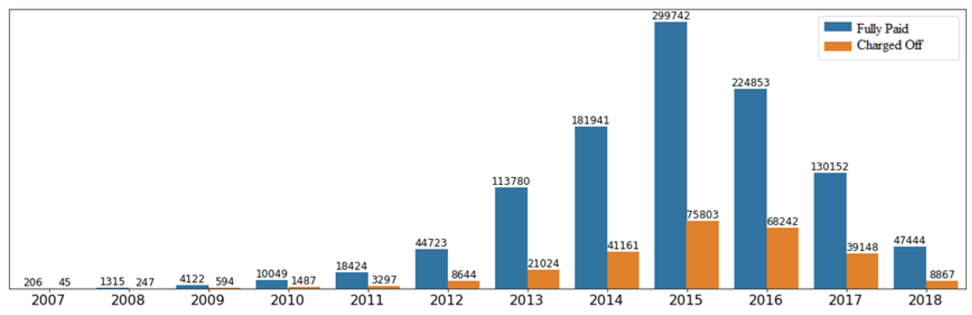
4.1. Overview
4.2. Data Pre-Processing
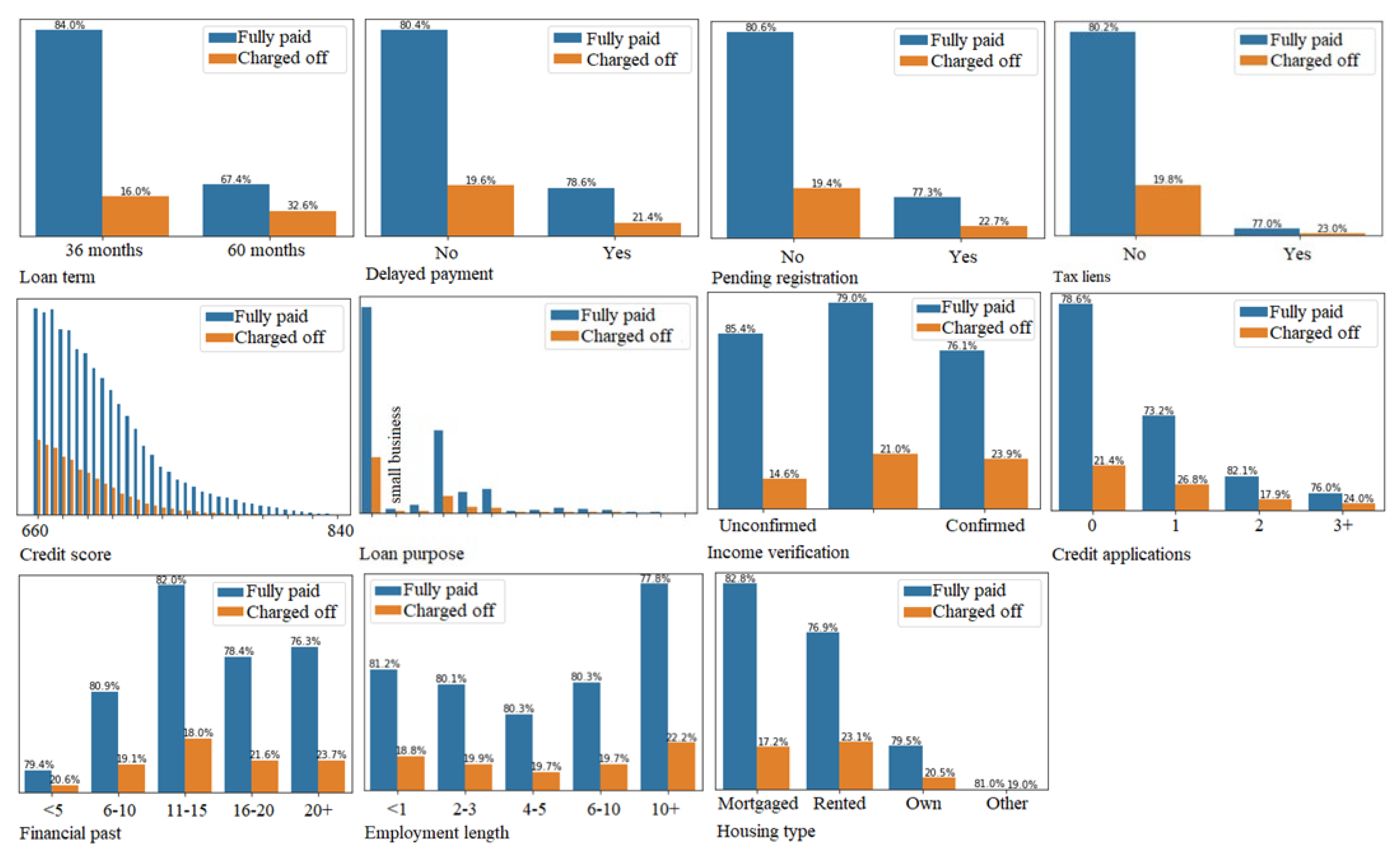
4.3. Exploratory Data Analysis
5. Experimental Results
5.1. Experiment Design
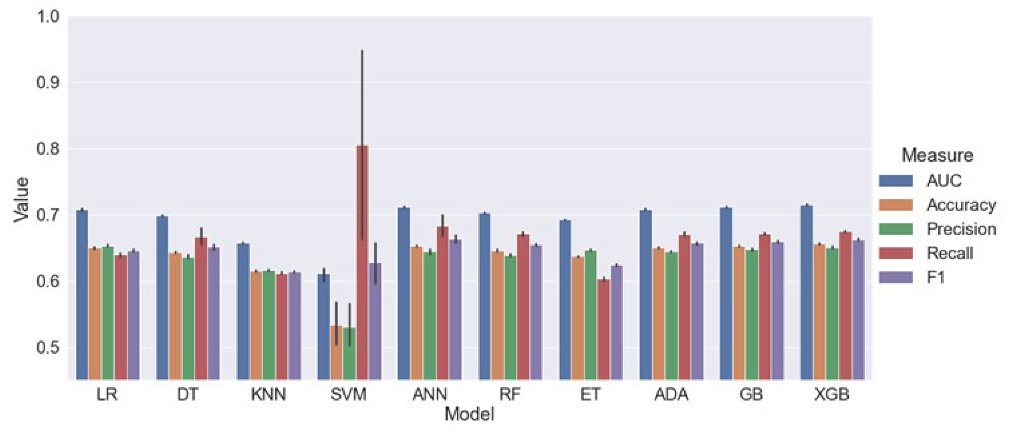
5.2. General Results
5.3. Hyperparameter Optimization and Final Evaluation
5.4. Benchmarking Results and Practical Implications
6. Conclusions
Author Contributions
Funding
Data Availability Statement
Conflicts of Interest
References
- Abdou, Hussein A., and John Pointon. 2011. Credit scoring, statistical techniques and evaluation criteria: A review of the literature. Intelligent Systems in Accounting, Finance and Management 18: 59–88. [Google Scholar] [CrossRef]
- Araujo, Fabio. 2022. Initial Steps towards a Central Bank Digital Currency by the Central Bank of Brazil. BIS Papers No. 123. pp. 31–37. Available online: https://www.bis.org/publ/bppdf/bispap123.pdf (accessed on 15 November 2023).
- Athey, Susan, and Guido W. Imbens. 2019. Machine learning methods that economists should know about. Annual Review of Economics 11: 685–725. [Google Scholar] [CrossRef]
- Bali, Turan G., Heiner Beckmeyer, Mathis Moerke, and Florian Weigert. 2023. Predicting option returns with machine learning and big data. Review of Financial Studies 36: 3548–602. [Google Scholar] [CrossRef]
- Bazarbash, Majid. 2019. FinTech in Financial Inclusion: Machine Learning Applications in Assessing Credit Risk. IMF Working Paper No. 2019/109. Available online: https://www.imf.org/-/media/Files/Publications/WP/2019/WPIEA2019109.ashx (accessed on 15 November 2023).
- Berg, Tobias, Valentin Burg, Ana Gombović, and Manju Puri. 2020. On the rise of FinTechs: Credit scoring using digital footprints. Review of Financial Studies 33: 2845–97. [Google Scholar] [CrossRef]
- Bergstra, James, and Yoshua Bengio. 2012. Random search for hyper-parameter optimization. Journal of Machine Learning Research 13: 281–305. Available online: https://dl.acm.org/doi/pdf/10.5555/2188385.2188395 (accessed on 15 November 2023).
- Bishop, Christopher M. 2006. Pattern Recognition and Machine Learning. Berlin: Springer Nature B.V. [Google Scholar]
- Breiman, Leo. 2001. Statistical modeling: The two cultures. Statistical Science 16: 199–231. [Google Scholar] [CrossRef]
- Cakici, Nusret, Christian Fieberg, Daniel Metko, and Adam Zaremba. 2023. Do anomalies really predict market returns? New data and new evidence. Review of Finance. Forthcoming. Available online: https://ssrn.com/abstract=4557747 (accessed on 15 November 2023).
- Chakraborty, Chiranjit, and Andreas Joseph. 2017. Machine Learning at Central Banks. Bank of England Working Paper No. 674. Available online: https://www.bankofengland.co.uk/working-paper/2017/machine-learning-at-central-banks (accessed on 15 November 2023).
- Dastile, Xolani, Turgay Celik, and Moshe Potsane. 2020. Statistical and machine learning models in credit scoring: A systematic literature survey. Applied Soft Computing 91: 106263. [Google Scholar] [CrossRef]
- Drobetz, Wolfgang, Fabian Hollstein, Tizian Otto, and Marcel Prokopczuk. 2021. Estimating stock market betas via machine learning. SSRN. [Google Scholar] [CrossRef]
- Dua, Dheeru, and Casey Graff. 2017. UCI Machine Learning Repository. University of California, Irvine, School of Information and Computer Sciences. Available online: https://archive.ics.uci.edu/ml/index.php (accessed on 15 November 2023).
- Finlay, Steven. 2011. Multiple classifier architectures and their application to credit risk assessment. European Journal of Operational Research 210: 368–78. [Google Scholar] [CrossRef]
- George, Nathan. 2018. All Lending Club Loan Data. Available online: https://www.kaggle.com/wordsforthewise/lending-club (accessed on 15 November 2023).
- Gu, Shihao, Bryan Kelly, and Dacheng Xiu. 2020. Empirical asset pricing via machine learning. Review of Financial Studies 33: 2223–73. [Google Scholar] [CrossRef]
- Hand, David J., and William E. Henley. 1997. Statistical classification methods in consumer credit scoring: A review. Journal of the Royal Statistical Society: Series A (Statistics in Society) 160: 523–41. [Google Scholar] [CrossRef]
- Lessmann, Stefan, Bart Baesens, Hsin-Vonn Seow, and Lyn C. Thomas. 2015. Benchmarking state-of-the-art classification algorithms for credit scoring: An update of research. European Journal of Operational Research 247: 124–36. [Google Scholar] [CrossRef]
- Louzada, Francisco, Anderson Ara, and Guilherme B. Fernandes. 2016. Classification methods applied to credit scoring: Systematic review and overall comparison. Surveys in Operations Research and Management Science 21: 117–34. [Google Scholar] [CrossRef]
- Malekipirbazari, Milad, and Vural Aksakalli. 2015. Risk assessment in social lending via random forests. Expert Systems with Applications 42: 4621–31. [Google Scholar] [CrossRef]
- Markov, Anton, Zinaida Seleznyova, and Victor Lapshin. 2022. Credit scoring methods: Latest trends and points to consider. The Journal of Finance and Data Science 8: 180–201. [Google Scholar] [CrossRef]
- Serrano-Cinca, Carlos, Begoña Gutiérrez-Nieto, and Luz López-Palacios. 2015. Determinants of default in P2P lending. PLoS ONE 10: e0139427. [Google Scholar] [CrossRef] [PubMed]
- Teply, Petr, and Michal Polena. 2020. Best classification algorithms in peer-to-peer lending. North American Journal of Economics and Finance 51: 100904. [Google Scholar] [CrossRef]
- Varian, Hal R. 2014. Big data: New tricks for econometrics. Journal of Economic Perspectives 28: 3–28. [Google Scholar] [CrossRef]
- Vicente, Julia. 2020. Fintech disruption in Brazil: A study on the impact of open banking and instant payments in the Brazilian financial landscape. Social Impact Research Experience 86. Available online: https://repository.upenn.edu/sire/86 (accessed on 15 November 2023).
- Wu, Xindong, Vipin Kumar, J. Ross Quinlan, Joydeep Ghosh, Qiang Yang, Hiroshi Motoda, Geoffrey J. McLachlan, Angus Ng, Bing Liu, Philip S. Yu, and et al. 2008. Top 10 algorithms in data mining. Knowledge and Information Systems 14: 1–37. [Google Scholar] [CrossRef]
- Xia, Yufei, Lingyun He, Yinguo Li, Nana Liu, and Yanlin Ding. 2020. Predicting loan default in peer-to-peer lending using narrative data. Journal of Forecasting 39: 260–80. [Google Scholar] [CrossRef]
- Zhang, Xiaoming, and Lean Yu. 2024. Consumer credit risk assessment: A review from the state-of-the-art classification algorithms, data traits, and learning methods. Expert Systems with Applications 237: 121484. [Google Scholar] [CrossRef]
- Zhou, Xianzheng, Hui Zhou, and Huaigang Long. 2023. Forecasting the equity premium: Do deep neural network models work? Modern Finance 1: 1–11. [Google Scholar] [CrossRef]


| Paper | Sample | n | Features | Algorithm | Performance Metric |
|---|---|---|---|---|---|
| Serrano-Cinca et al. 2015 | 2008–2011 | 3788 | 5 | Logistic regression | Accuracy Hosmer–Lemeshow test Nagelkerke’s R2 |
| Malekipirbazari and Aksakalli 2015 | 2012–2014 | 68,000 | 15 | Logistic regression K-nearest neighbors Random forests Support vector machines | Accuracy Area under the curve Root mean square error |
| Xia et al. 2020 | 2011–2013 | 64,139 | 15 | Logistic regression Decision tree Random forests Artificial neural networks Gradient boosting decision tree XGBoost CatBoost | Accuracy False positive rate False negative rate Area under the curve Hirsch index |
| This work | 2007–2018 | 1,305,402 | 18 | Logistic regression Decision tree K-nearest neighbors Support vector machines Artificial neural networks Random forests Extra trees AdaBoost Gradient boosting decision tree XGBoost | Accuracy Precision Recall F1-score Area under the curve |
| Predicted | ||
|---|---|---|
| Observed | Charged-off | Fully paid |
| Charged-off | TP | FN |
| Fully paid | FP | TN |
| Feature | Description | Type |
|---|---|---|
| Annual income | Self-reported by the loan applicant in US dollars at the time of registration | Numeric |
| Debt-to-income ratio | Monthly debt payments (excluding mortgages and the sought loan) as a percentage of monthly income | Numeric |
| Limit surpassed | Ratio between the amount of credit the borrower is using and all available revolving credit (e.g., credit cards) | Numeric |
| Credit availability | Total number of open credit lines reflected in the borrower’s credit file | Numeric |
| Banking partnership | Total number of credit lines currently in the borrower’s credit file | Numeric |
| Financial past | Time, in years, after the borrower opened his or her first credit line until the time of the request | Categorical (possible values: up to 5 years, 6–10 years, 11–15 years, 16–20 years, and over 20 years) |
| Credit score | The value of the lower limit of the borrower’s score range (FICO® Score) at the time of the request | Numeric |
| Delayed payments | Indicator of the existence of payment commitments that are more than 30 days past due in the recent two years | Categorical (possible values: yes or no) |
| Credit applications | Number of credit inquiries in the last six months, excluding autos and mortgages | Categorical (possible values: 0, 1, 2, 3 or 3+) |
| Pending registration | Indicator of the presence of derogatory public records | Categorical (possible values: yes or no) |
| Tax liens | Indicator of the existence of outstanding tax issues in the borrower’s history | Categorical (possible values: yes or no) |
| Employment length | Employment length in years | Categorical (possible values: up to 1 year, 2–3 years, 4–5 years, 6–10 years, 10+ years) |
| Housing type | Housing situation of the borrower at the time of application | Categorical (possible values: own, mortgaged, rented, other) |
| Income verification | Validation indicator of the borrower’s informed worth or source of income at the time of the request | Categorical (possible values: verified, not verified, verified source) |
| Loan amount | The loan application in US dollars | Numeric |
| Loan interest rate | The loan’s annual interest rate | Numeric |
| Loan term | Total loan term expressed in months | Categorical (possible values: 36 or 60 months) |
| Loan purpose | The borrower’s chosen purpose or objective for the loan at the time of application | Categorical (possible values: debt restructuring, credit card, remodeling, purchases, health, small business, vehicle, moving, vacation, property, marriage, renewable energy, education, other) |
| Annual Income | Debt-to-Income Ratio, % | Limit Surpassed, % | Credit Availability | Banking Partnership | Loan Amount | Loan Interest Rate, % | |
|---|---|---|---|---|---|---|---|
| Mean | 73.13 | 18.1 | 51.85 | 11.57 | 24.93 | 14.21 | 13.23 |
| S.D. | 38.55 | 8.35 | 24.44 | 5.42 | 11.91 | 8.57 | 4.75 |
| Minimum | 2 | 0 | 0 | 0 | 2 | 0.5 | 5.31 |
| 25% | 46 | 11.85 | 33.5 | 8 | 16 | 7.75 | 9.75 |
| 50% | 65 | 17.61 | 52.2 | 11 | 23 | 12 | 12.74 |
| 75% | 90 | 23.97 | 70.7 | 14 | 32 | 20 | 15.99 |
| Maximum | 252.4 | 49.96 | 193 | 40 | 80 | 40 | 30.99 |
| Algorithm | Hyperparameter |
|---|---|
| Logistic regression (LR) | class_weight=“balanced” |
| Decision tree (DT) | algorithm=CART, class_weight=“balanced”, max_depth=7, min_samples_leaf=0.01 |
| K-nearest neighbors (KNN) | n_neighbors=11 |
| Support vector machines (SVM) | kernel=“rbf”, class_weight=“balanced”, max_iter=100,000 |
| Artificial neural networks (ANN) | hidden_layer_sizes=(8,4), activation=“relu”, solver=“adam”, learning_rate= 0.001(“constant”) |
| Random forests (RF) | class_weight=“balanced”, max_depth=7, min_samples_leaf=0.01 |
| Extra trees (ET) | class_weight=“balanced”, max_depth=7, min_samples_leaf=0.01 |
| AdaBoost (ADA) | algorithm= SAMME.R |
| Gradient boosting (GB) | loss=“log_loss”, learning_rate=0.1, n_estimators=100, max_depth=3, min_samples_leaf=1 |
| XGBoost (XGB) | booster=gbtree, learning_rate=0.3, gamma=0, alpha=0, min_child_weight=1, max_depth=6, sampling_method=uniform |
| Model | AUC | Accuracy | Precision | Recall | F1 | Time * (s) |
|---|---|---|---|---|---|---|
| Logistic regression (LR) | 0.7087 [0.0019] | 0.6568 [0.0013] | 0.3205 [0.0026] | 0.6403 [0.0037] | 0.4272 [0.0030] | 14.0 |
| Decision tree (DT) | 0.6998 [0.0018] | 0.6167 [0.0076] | 0.3003 [0.0039] | 0.6896 [0.0104] | 0.4183 [0.0027] | 8.0 |
| K-nearest neighbors (KNN) | 0.6438 [0.0012] | 0.7921 [0.0007] | 0.4176 [0.0048] | 0.1028 [0.0016] | 0.1650 [0.0023] | 7806.0 |
| Support vector machines (SVM) | 0.5488 [0.0078] | 0.3759 [0.0546] | 0.2012 [0.0035] | 0.7127 [0.0762] | 0.3130 [0.0061] | 18,453.0 |
| Artificial neural networks (ANN) | 0.7141 [0.0018] | 0.8031 [0.0010] | 0.5640 [0.0115] | 0.0640 [0.0033] | 0.1149 [0.0052] | 43.0 |
| Random forests (RF) | 0.7032 [0.0012] | 0.6283 [0.0022] | 0.3058 [0.0025] | 0.6773 [0.0030] | 0.4214 [0.0026] | 91.0 |
| Extra trees (ET) | 0.6919 [0.0011] | 0.6496 [0.0005] | 0.3098 [0.0019] | 0.6138 [0.0020] | 0.4118 [0.0020] | 69.0 |
| AdaBoost (AB) | 0.7087 [0.0013] | 0.8023 [0.0010] | 0.5439 [0.0063] | 0.0657 [0.0052] | 0.1172 [0.0082] | 83.0 |
| Gradient boosting (GB) | 0.7128 [0.0017] | 0.8029 [0.0009] | 0.5637 [0.0080] | 0.0610 [0.0006] | 0.1101 [0.0011] | 351.0 |
| XGBoost (XGB) | 0.7185 [0.0015] | 0.8036 [0.0010] | 0.5549 [0.0081] | 0.0857 [0.0019] | 0.1484 [0.0031] | 52.0 |
| Model | AUC | Accuracy | Precision | Recall | F1 | Time * (s) |
|---|---|---|---|---|---|---|
| Logistic regression (LR) | 0.7076 [0.0015] | 0.6499 [0.0017] | 0.6531 [0.0020] | 0.6393 [0.0031] | 0.6461 [0.0024] | 5.6 |
| Decision tree (DT) | 0.6988 [0.0013] | 0.6431 [0.0016] | 0.6366 [0.0031] | 0.6670 [0.0139] | 0.6513 [0.0053] | 2.8 |
| K-nearest neighbors (KNN) | 0.6572 [0.0013] | 0.6150 [0.0012] | 0.6157 [0.0012] | 0.6119 [0.0019] | 0.6138 [0.0013] | 1327.4 |
| Support vector machines (SVM) | 0.6111 [0.0117] | 0.5335 [0.0362] | 0.5309 [0.0378] | 0.8060 [0.1709] | 0.6279 [0.0353] | 6951.2 |
| Artificial neural networks (ANN) | 0.7116 [0.0018] | 0.6527 [0.0017] | 0.6440 [0.0048] | 0.6837 [0.0181] | 0.6631 [0.0063] | 33.7 |
| Random forests (RF) | 0.7026 [0.0008] | 0.6459 [0.0015] | 0.6390 [0.0025] | 0.6709 [0.0039] | 0.6545 [0.0019] | 32.2 |
| Extra trees (ET) | 0.6925 [0.0008] | 0.6369 [0.0009] | 0.6468 [0.0011] | 0.6030 [0.0035] | 0.6241 [0.0022] | 26.3 |
| AdaBoost (ADA) | 0.7078 [0.0012] | 0.6500 [0.0011] | 0.6441 [0.0014] | 0.6704 [0.0030] | 0.6570 [0.0019] | 31.0 |
| Gradient boosting (GB) | 0.7118 [0.0010] | 0.6531 [0.0016] | 0.6476 [0.0022] | 0.6717 [0.0015] | 0.6594 [0.0018] | 130.0 |
| XGBoost (XGB) | 0.7153 [0.0013] | 0.6563 [0.0018] | 0.6507 [0.0022] | 0.6749 [0.0019] | 0.6626 [0.0020] | 16.5 |
| Model | AUC | Accuracy | Precision | Recall | F1 |
|---|---|---|---|---|---|
| XGBoost (XGB) | 1 | 1 | 2 | 3 | 2 |
| Gradient boosting (GB) | 2 | 2 | 3 | 4 | 3 |
| Artificial neural networks (ANN) | 3 | 3 | 6 | 2 | 1 |
| AdaBoost (ADA) | 4 | 4 | 5 | 6 | 4 |
| Logistic regression (LR) | 5 | 5 | 1 | 8 | 7 |
| Random forests (RF) | 6 | 6 | 7 | 5 | 5 |
| Decision tree (DT) | 7 | 7 | 8 | 7 | 6 |
| Extra trees (ET) | 8 | 8 | 4 | 10 | 9 |
| K-nearest neighbors (KNN) | 9 | 9 | 9 | 9 | 10 |
| Support vector machines (SVM) | 10 | 10 | 10 | 1 | 8 |
| Hyperparameter | Value Grid | Optimal Value |
|---|---|---|
| max_depth | [3, 6, 8, 10, 12, 15, 20] | 6 |
| min_child_weight | [1, 3, 5, 7, 10] | 1 |
| gamma | [0, 0.0001, 0.001, 0.01, 0.1] | 0.001 |
| learning_rate | [0.01, 0.05, 0.1, 0.2, 0.3, 0.5] | 0.3 |
| alpha | [0, 0.0001, 0.001, 0.01, 0.1] | 0.01 |
| subsample | [0.1, 0.25, 0.5, 0.75, 1] | 1 |
| colsample_bytree | [0.1, 0.25, 0.5, 0.75, 1] | 0.75 |
| colsample_bylevel | [0.1, 0.25, 0.5, 0.75, 1] | 0.75 |
| colsample_bynode | [0.1, 0.25, 0.5, 0.75, 1] | 1 |
| Class | Precision | Recall | F1 |
|---|---|---|---|
| Fully paid loan (0) | 0.8880 | 0.6393 | 0.7434 |
| Charged-off loan (1) | 0.3151 | 0.6729 | 0.4292 |
| Macro | 0.6015 | 0.6561 | 0.5863 |
| Balanced | 0.7746 | 0.6459 | 0.6812 |
| Accuracy | 0.6459 |
Disclaimer/Publisher’s Note: The statements, opinions and data contained in all publications are solely those of the individual author(s) and contributor(s) and not of MDPI and/or the editor(s). MDPI and/or the editor(s) disclaim responsibility for any injury to people or property resulting from any ideas, methods, instructions or products referred to in the content. |
© 2023 by the authors. Licensee MDPI, Basel, Switzerland. This article is an open access article distributed under the terms and conditions of the Creative Commons Attribution (CC BY) license (https://creativecommons.org/licenses/by/4.0/).
Share and Cite
Suhadolnik, N.; Ueyama, J.; Da Silva, S. Machine Learning for Enhanced Credit Risk Assessment: An Empirical Approach. J. Risk Financial Manag. 2023, 16, 496. https://doi.org/10.3390/jrfm16120496
Suhadolnik N, Ueyama J, Da Silva S. Machine Learning for Enhanced Credit Risk Assessment: An Empirical Approach. Journal of Risk and Financial Management. 2023; 16(12):496. https://doi.org/10.3390/jrfm16120496
Chicago/Turabian StyleSuhadolnik, Nicolas, Jo Ueyama, and Sergio Da Silva. 2023. "Machine Learning for Enhanced Credit Risk Assessment: An Empirical Approach" Journal of Risk and Financial Management 16, no. 12: 496. https://doi.org/10.3390/jrfm16120496
APA StyleSuhadolnik, N., Ueyama, J., & Da Silva, S. (2023). Machine Learning for Enhanced Credit Risk Assessment: An Empirical Approach. Journal of Risk and Financial Management, 16(12), 496. https://doi.org/10.3390/jrfm16120496