Spreads and Volatility in House Returns

Abstract

Underlying idiosyncratic and illiquidity risks are suppressed in infrequently reported indexes of house prices and rents. Idiosyncratic risks result from bid–ask spreads for prices and rents. Time series autocovariances generate a distribution of prices and rents. Capital gains and rent-price ratios are transforms of these distributions, generating cross-sectional idiosyncratic volatility. Housing data are infrequent and usually made available every month. The monthly–quarterly volatility ratios of house prices and rents and their spreads estimate unobserved daily fluctuations and illiquidity risks. Including idiosyncratic and illiquidity risks, a U.S. house has a standard deviation in returns of 8.7% annually for three decades after 1990. With a mean excess return of 3.7%, the Sharpe ratio of 0.42 is comparable to the S&P 500. Excluding spreads, the house Sharpe ratio is 0.69. House returns respond to liquidity. A 1% increase in volume raises returns by 0.8%.

1. Introduction

This paper measures underlying idiosyncratic and illiquidity risks that are suppressed in the infrequently reported index numbers of house prices and rents. The method involves Roll (1984) bid–ask spreads for prices and rents. Buyers are paying different prices for comparable houses at the same time. Tenants are paying different rent prices in the same market. Time-series autocovariances generate a distribution of prices and rent that participants face at a given time. Capital gains and rent-price ratios are transforms of these distributions, allowing for an added cross-sectional standard deviation in returns. This is an idiosyncratic risk of housing generated from bid–ask spreads at a given time.

There are two differences between houses and financial assets that are suppressed. One is that different buyers of S&P 500 simultaneously earn identical returns with minimal spreads. Different buyers or renters of a house at the same time face separate prices and rents.

The other is that while houses and stocks trade daily, reporting differs. Housing data are infrequent and usually made available every month. Stock trading is continuous but reported daily. Data reported on houses are at a lower frequency than for financial assets and are reported in a monthly manner. Aggregate data are usually reported as an index. To construct the return to holding a house relies on using these index number-based, monthly series. The monthly–quarterly volatility ratios of house prices and rents provide implicit estimates of unobserved daily fluctuations and illiquidity risks.

This paper proposes adjustments of price and rent series to incorporate idiosyncratic and illiquidity risks. The method derives bid–ask spreads for rent and prices. As in Roll (1984), Abdi and Ranaldo (2017) and Hagstromer (2021), the spreads or price and rent ranges are based on first-order autocovariances. These are observable directly in the time series. The spreads derive cross-sectional volatilities in returns from those on rent and prices for the monthly data. There is a cross-sectional distribution of returns, measuring the idiosyncratic risk.

These monthly volatilities in prices, rent, and returns are computed quarterly. The monthly–quarterly volatility ratios provide an estimate of the time smoothing of risk. The time-smoothing estimate is applied to derive an implicit daily volatility, which is a measure of the housing market’s illiquidity.

Together with a conversion of prices and rent in index form to currency, the procedures allow housing returns to be constructed with data as reported. These procedures allow for the construction of aggregate performance of the housing market.

These procedures are applied on monthly U.S. data for the three decades since 1990. Rent is the homeowner equivalent in the Consumer Price Index, as reported by the Bureau of Labor Statistics. Prices are the repeat-sales purchase-only index from the Federal Housing Finance Administration. The conversion to currency uses Census benchmarks, controlled to the monthly index performance.

With currency data and an estimate of operating expenses, a house’s cap rate is derived monthly. This is the yield or net operating income per USD of the price. The yield plus the capital gain from the FHFA series is the total return on holding a house. The excess return is the net of the yield to maturity on 90-day Treasury bills.

The annualized mean excess return is 3.7%. The standard deviation is 5.4% annually. The Sharpe ratio is 0.69. The comparable Sharpe ratio for S&P 500 is 0.40 and with a standard deviation of returns of 18.2% annually. A house earns a risk-adjusted return more than 50% greater than a stock index with a fraction of the volatility.

The cross-sectional idiosyncratic risk from the bid–ask spread adds 2.0% annually to a house’s volatility. The illiquidity risk from temporal smoothing adds 1.3% annually. In both cases, the mean excess return remains unchanged. With these two risks included, the annual volatility of house returns becomes 8.7% annually. The Sharpe ratio becomes 0.42. A house moves from being above the efficient risk-return frontier to being along it.

The results control for volume. There is a positive volume–return relationship. A 1% increase in volume leads to a 0.8% increase in expected excess returns to holding a house.

Housing data are reported monthly and in index form. To convert the data into return series, three steps are proposed. The first converts the prices and rents from indexes to currency. These currency rents and prices allow the construction of a return series. The second step derives bid–ask spreads for rent and prices from their autocovariances. These result in volatilities of rent, prices and returns cross-sectionally. In the third step, volatilities at different time intervals estimate illiquidity risks.

2. Background

Households pay different prices and rent for houses at the same time. They are constrained in diversification given the cost of houses relative to representative income and fungible wealth. Averaging with an overall index removes this cross-sectional volatility.

Real estate prices decline when expected financial asset risks increase (Fan et al. 2013). Housing is related to consumption through the wealth effect. The marginal propensity of consumption from housing wealth ranges from 6 to 10 cents on the dollar annually in the United States. It is greater in China (Chen et al. 2020) given the dominance of real estate in household portfolios. Cheng et al. (2021) examined the performance of reservation and number rules as selling strategies in housing. Real estate returns vary across countries, although they are tied to a market property index (Bond et al. 2003). Housing wealth accumulation depends on socioeconomic factors, including the number of children in a household and the household’s gender composition (Hardin et al. 2022).

Properties sell for different prices at the same time. Attributes that have a high value at a location or property type have a lower estimate elsewhere (Prashant et al. 2018). Less expensive properties have different hedonic prices of characteristics than higher-end ones.

Agents selling their own houses achieve 3.7% higher prices, although at a cost of staying on the market for a longer period of time (Levitt and Syverson 2005). Within clients, prices are lower for properties owned by firms than individuals (Xie 2018). These properties include distress and foreclosure sales. A part of the spread is an externality formed in neighborhoods. A nearby foreclosure leads to price declines in the neighborhood (Lin et al. 2009). In Xie (2022), a network rather than a random search is more valuable in finding a transaction match.

There are idiosyncratic risks at the household level. Using Case–Shiller individual data, Flavin and Yamashita (2002) observed a house inflation standard deviation of 7% annually. In Landvoigt et al. (2015), annual house inflation volatility averaged 9% in San Diego and 15% in Los Angeles (Giacoletti and Westrupp 2017).

House prices increase with leverage (Genesove and Mayer 1997) and decrease for lenders and estate sellers (Campbell et al. 2011). House prices vary regionally (Hurst et al. 2016), seasonally (Kotova and Zhang 2020) and depend on local bank finances (Cloyne et al. 2019; Blickle 2022).

There has been an examination of spreads in the distribution of house prices and rent. Buttimer et al. (1997) evaluated the pricing of mortgage securities when prices are based on an index. Swap spreads for property index contracts are greater than those predicted by models (Pu et al. 2012). The objective of this paper is to address idiosyncratic risks by incorporating distributions of rents and prices at each date. A joint rent–price distribution is developed.

Spreads for rents and prices as in Roll (1984), Hasbrouck (2009), Corwin and Schultz (2012) and Abdi and Ranaldo (2017) are based on their autocovariances. Hagstromer (2021) indicates that using the midpoint leads to a bias that potentially overstates the bid–ask spread. Instead, a weighted midpoint incorporates liquidity distributions within the spread. The midpoint is the average of the bid and ask prices. The weighted midpoint uses a fraction of the volume or depth available at the bid and ask prices. The cross-covariances between rent and price inflation are not restricted to zero. The covariance matrix between rent and house price inflation generates their cross-sectional distributions.

A lack of liquidity reduces house volumes and prices. In Krainer (2001), a liquid market with looser mortgage underwriting increases the cost of not closing, driving up prices. A hot, liquid market has increasing volumes and prices. Kotova and Zhang (2020) observed narrower spreads during seasonally hot housing markets in the summer.

Giacoletti (2021) constructs end-to-end returns for buying and selling a house, including improvements. Instead of errors proportionate in the time period held, their absolute value jumps in early years and then flattens. Sagi (2021) follows commercial properties held by institutional investors in the National Council of Real Estate Investment Fiduciaries. Return errors follow similar failures relative to a random walk with drift. Idiosyncratic risks emerge as a pricing factor for housing returns in Eiling et al. (2021).

The structure includes volume in estimations to test housing’s unique liquidity. There is a price–volume correlation. Volume has no scaling by returns or prices. The liquidity risk from infrequent trading uses variance ratios. The estimation of the covariance matrix is for available monthly data, and the data are re-estimated quarterly. The ratio of the monthly-to-quarterly variance measures the risk of infrequent trading. A higher ratio at the lower frequency confirms this liquidity risk. The variance ratio allows for an implicit estimate of the unobserved daily volatility of rent, prices and their covariances. The daily variances render a house comparable with financial assets.

Volume has a separate liquidity risk. The cross-sectional volatility for non-diversification, the variance ratio for infrequent trading intervals and volume are factors in asset pricing a house.

From the Federal Reserve Board’s Survey of Consumer Finances, homeowners hold undiversified portfolios, largely containing a principal residence. The results are robust between the 2016 and 2019 Surveys (Bhutta et al. 2020) and the 2013 and 2016 surveys (Bricker et al. 2017). In Goetzmann et al. (2021), privately held assets have a capital stock three times that of GDP. Housing and commercial real estate are each one-third of this stock.

The return is the sum of real capital gains and a dividend yield from the net rent divided by the house price. During 1890–2020 for U.S. houses, from Shiller (2015, 2021), real house capital gains are 0.5% annually. With a 2.4% net rent-price dividend yield, the mean annual real return to holding a house is 2.9%. The estimate is obtained by converting Case–Shiller prices and the Bureau of Labor Statistics rent to currency (Davis et al. 2008) and subtracting operating expenses using National Apartment Association expense ratios, over 1968–2020.

Long-run housing returns have been constructed including in endowments in Chambers et al. (2021). Housing responds to macro-fluctuations in Burnside et al. (2016). During booms, there is the added entry of real estate agents. These entrants have lower post-boom wages relative to those entering in slower markets (Begley et al. 2022). In some cases, repeat transactions allow for the procedures of Case and Shiller (1989).

The long-run real return to holding property is 2.6% annually from 99-year U.K. leases (Giglio et al. 2021). The volatility of returns is modest when using an aggregate index such as in the United States. Those widely used are from S&P/CoreLogic/Case-Shiller and Federal Housing Finance Administration in prices and residential rent from the Consumer Price Index. Ghysels et al. (2013, Table 2) report standard deviations of 2.0% for FHFA, 2.9% for Case–Shiller equally weighted and 3.3% for a 10-city index over 1980–2007. The rent–price ratio from the Lincoln Land Institute has a standard deviation of 1.6% annually.

3. Cross-Sectional Prices and Rents

Transactions on houses are bilateral and diffused, leading to current-time variations on rent and prices and idiosyncratic risks. Financing requirements and required inspections slow transaction speeds. Transactions are infrequent, introducing liquidity risks. Aggregate data smooth out these cross-sectional and liquidity risks.

At time $t$, the price of a house is $H_t$. The price is from an overall index. The date $t$ is at a reporting frequency that is less than in financial markets, such as monthly reporting. The house generates net rent $R_t$. Net rent is obtained after operating expenses for property taxes, insurance and maintenance. The logarithm of the price is $h_t=ln{H}_t$. The logarithm of the net rent is $r_t=ln{R}_t$. The single reported price $h_t$ is from a distribution that buyers and sellers are facing and paying. The imputed rent is distributed around $r_t$.

Households form expectations about house prices ${\tilde{h}}_t$ and rent ${\tilde{r}}_t$. The expectations on house price and rent appreciation are $\Delta {\tilde{h}}_t \mathrm{and}\Delta {\tilde{r}}_t$. Rent and price levels compare with expectations as follows.

$$\{\begin{array}{c}{r}_t={\tilde{r}}_t+{\epsilon }_{rt}\\ h_t={\tilde{h}}_t+{\epsilon }_{ht}\end{array}.$$

(1)

The error in rent is ${\epsilon }_{rt}$. The error in house prices is ${\epsilon }_{ht}$.

The return to a house involves linear combinations of (1). Capital gains are the first difference in logarithmic prices $\Delta h_t$. The risks are $var(\Delta h_t)$ and $var(\Delta r_t)$. The dividend yield is the first difference between logarithmic rents and prices $r_t-h_t$. The yield’s risk is from its variance $var(r_t-h_t)$. There is a covariance between rent and house prices in the yield. Another covariance is between the rental dividend and house appreciation.

Inflationary expectations for house prices and rents are $\Delta {\tilde{h}}_t$ and $\Delta {\tilde{r}}_t$. Appreciation in house prices and rents are at the following rates.

$$\{\begin{array}{c}\Delta r_t=\Delta {\tilde{r}}_t+{\upsilon }_{rt}\\ \Delta h_t=\Delta {\tilde{h}}_t+{\upsilon }_{ht}\end{array}.$$

(2)

The capital gain is $\Delta h_t$. The expected capital gain is $\Delta {\tilde{h}}_t$. The error in house capital gains is ${\upsilon }_{pt}=\Delta {\epsilon }_{pt}$. Rental appreciation is $\Delta r_t$. Households expect rent growth to be $\Delta {\tilde{r}}_t$. The actual-minus-expected rent error is ${\upsilon }_{pt}=\Delta {\epsilon }_{rt}$.

The return to holding a house is as follows.

$$x_t=\Delta ln{\tilde{H}}_t+{\tilde{R}}_t/{\tilde{H}}_t+{\epsilon }_{xt}.$$

(3)

The expected rent and price levels are ${\tilde{R}}_t=\exp ({\tilde{r}}_t)$ and ${\tilde{H}}_t=\exp ({\tilde{h}}_t).$ The return has an expected capital gain $\Delta {\tilde{h}}_t$. The expected dividend yield is ${\tilde{R}}_t/{\tilde{H}}_t$. The return’s error is ${\epsilon }_{xt}$. An owner has risks of capital gains or losses and dividends. The risk for owners is as follows.

$$\{\begin{array}{c}var(\Delta h_t)=var(\Delta {\tilde{h}}_t)+var({\upsilon }_{ht})+2cov(\Delta {\tilde{p}}_h,{\upsilon }_{ht})\\ var(r_t-h_t)=var({\tilde{r}}_t)-var({\tilde{h}}_t)+var({\epsilon }_{rt}-{\epsilon }_{ht})-2cov(r_t,h_t)\end{array}.$$

(4)

These measures as reported monthly are sufficient when housing has no liquidity risk from infrequent unobserved daily trading.

Liquidity risk comes from houses being traded at low frequencies. Daily trading at frequency $d$ is not available for houses. The reported $t$ averages over infrequent trading periods, suppressing volatility. The time measures are for $t$ with houses trading less frequently than financial assets. Liquidity risks add to those for the overall market and idiosyncrasies.

The variances $var(\Delta {\tilde{r}}_t)$ and $var(\Delta {\tilde{h}}_t)$ are for market volatility with one observation per period. Expected rents and house prices have variances $var({\tilde{r}}_t)$ and $var({\tilde{h}}_t)$. The idiosyncratic risks of tenants paying different rents and homeowners varying prices are $var({\upsilon }_{rt})$ and $var({\upsilon }_{ht})$. Homeowners for the same house have different rental yields, such as $var({\epsilon }_{rt}-{\epsilon }_{ht})$. Given the expense of holding a portfolio and that a household only occupies one house at a time, this risk is not diversifiable.

Rent has low volatility compared with prices, so these estimates are bound to the return volatility described above. Between one-quarter and one-half of tenants in single-family houses receive no rent increases upon a 12-month renewal (Genesove 2003; Gallin and Verbrugge 2019). Homeowners increase consumption when house prices increase, but renters do not (Aladangady 2017). Renters switch to owning when Facebook friends experience price increases, regardless of distance (Bailey et al. 2018).

The variances of expected rents and prices, with one observation per $t$, are $s_{\overline{r}}^2$ and $s_{\overline{h}}^2$. The market risk of a house is described as follows.

$$\{\begin{array}{c}var(\Delta {\tilde{h}}_t)=2s_{\overline{h}}^2 var({\tilde{r}}_t-{\tilde{h}}_t)=s_{\overline{r}}^2+s_{\overline{h}}^2-2cov({\tilde{r}}_t,{\tilde{h}}_t)\end{array}.$$

(5)

The homeowner’s market risk depends on overall capital gains $var(\Delta {\tilde{h}}_t)=2s_{\overline{h}}^2$ and relative rents and house prices $var({\tilde{r}}_t-{\tilde{h}}_t)=s_{\overline{r}}^2+s_{\overline{h}}^2-2cov({\tilde{r}}_t,{\tilde{h}}_t)$.

The idiosyncratic risk $var({\upsilon }_{rt})$ and $var({\upsilon }_{ht})$ from renting or owning one house has a cross-sectional covariance matrix $S=\left[\begin{array}{cc}{s}_h^2& s_{rh}\\ s_{rh}& s_r^2\end{array}\right]$. This matrix reflects the distribution of house prices and rent faced by households at a given time. Matrix $S$ shifts a distribution with mean zero and variance one in price errors for $h_t$ and $h_{t-1}$ and those for rent $r_t$ and $r_{t-1}$.

The idiosyncratic risk of a house is described as follows.

$$\{\begin{array}{c}var({\upsilon }_{rt})=2a_r^2 a_r^2=-cov(\Delta r_t,\Delta r_{t-1})\\ var({\upsilon }_{ht})=2a_h^2{a}_h^2=-cov(\Delta h_t,\Delta h_{t-1})\\ cov({\upsilon }_{rt},{\upsilon }_{ht})=2p_{\Delta r\Delta h}{a}_r^2{a}_h^2\\ var({\epsilon }_{rt}-{\epsilon }_{ht})=a_r^2+a_h^2-2p_{rh}{a}_r{a}_h\end{array}.$$

(6)

The correlation coefficient between rent and price levels is $p_{rh}$. The correlation coefficient between rent and price appreciation is $p_{\Delta r\Delta h}$. Homeowners are facing risks of prices and the imputed rent derived from tenants. Their risks include having paid different prices and that appreciation is not the same across houses. House prices and rent are logarithmic and symmetric. The central tendency including the mean or mode is its lag plus an error. The price is the mean plus the spread multiplied by a binary up-or-down shock with an absolute value one. The appreciation rates are the first differences in the errors plus the spreads multiplied by the changes in shock. The result is a set of covariances in house and rent appreciation and between them.

All the terms apply to a homeowner’s risk of holding one house. The contemporaneous rent–price covariance matrix is $S=\left[\begin{array}{cc}2a_r^2& p_{rh}{a}_r^2{a}_h^2\\ p_{rh}{a}_r^2{a}_h^2& 2a_h^2\end{array}\right]$. The variances of rent and price levels $a_r^2$, $a_h^2$ and the correlation coefficient $p_{rh}$ are flexible over time. The covariance matrix is cross-sectional, with households having different rent prices, house prices and appreciation at a point in time. A homeowner faces the risk of appreciation for rents and house prices that is different compared to neighbors or others around the country.

The last line $var({\epsilon }_{rt}-{\epsilon }_{ht})$ is for the dividend risk that homeowners face. This risk is based on how much the house rents for relative to its price, which varies across the market. The variances of cross-sectional rent and price levels are $a_r^2$ and $a_h^2$. With the rent–price correlation $p_{rh}$, the covariance term is $-2p_{rh}{a}_r{a}_h$.

In financial markets, there is a spread or range in prices (Roll 1984). The extension is to two variables for rents and prices and their covariance. The bid–ask spread as a transaction range depends on the negative of the first-order autocovariance of price growth. Hasbrouck (2009) uses Bayesian Gibbs estimation and imposes a non-negativity constraint.

Applied to the rent and price variances $a_r^2=\max (0,-cov(\Delta r_t,\Delta r_{t-1}))$ and $a_h^2=\max (0,-cov(\Delta h_t,\Delta h_{t-1})),$ liquidity risk has two components. One is from the error increasing at low holding lengths because of infrequent trading (Giacoletti 2021; Sagi 2021). The other is from volume-influencing prices but with a unique twist in housing markets. Volume-raising prices indicates liquidity for housing and not illiquidity (Krainer 2001).

Infrequent trading introduces a liquidity error. Daily frequency $d$ that data on financial markets report is unobserved. the less frequent monthly $t$ for housing markets is observed. Illiquidity raises the unobserved daily error relative to monthly reports, even after time scaling.

Analogous to d $var({\upsilon }_{rt})=2a_r^2$ and $var({\upsilon }_{ht})=2a_h^2$, the quarterly rent and price variances are $2q_r^2$ and $2q_h^2$. The quarterly estimates are from re-estimating the return and rental risk. The liquidity multiples or variance ratios for rents and prices are as follows:

$$\{\begin{array}{c}{m}_r^2(t)=\frac{a_r^2}{q_r^2}\\ m_h^2(t)=\frac{a_h^2}{q_h^2}\end{array}.$$

(7)

when $m_r(t), m_h(t)\le 1$, the volatility does not increase at a higher frequency of reporting. Scaling in the time argument takes into account the conversion from quarterly to monthly. Daily volatilities consistent with financial markets are $a_r^2{m}_r^2(d)$ and $a_h^2{m}_h^2(d)$. Here, $d$ is a month-to-day conversion factor. These are the implied daily variances annualized and they are adjusted for liquidity risks in rent and prices. They allow a house to be compared with financial assets including stocks and bonds.

The risk of holding a house for tenants and owners is described as follows.

$$\{\begin{array}{c}var(\Delta h_t)=var(\Delta {\tilde{h}}_t)+var({\upsilon }_{ht})=2s_{\overline{h}}^2+2a_h^2+m_h^2{a}_h^2\\ var(r_t-h_t)=s_{\overline{r}}^2+s_{\overline{h}}^2-2\rho s_{\overline{r}}^{ }{s}_{\overline{h}}^{ }+a_r^2(1+m_r^2)+a_h^2(1+m_h^2)\\ -2\rho a_r{a}_h(1+m_r^{ }{m}_h^{ })\end{array}.$$

(8)

The correlation between rents and prices is $\rho$. At the top is the risk of renting. Rent appreciation is the sum of risks for the market $2s_{\overline{r}}^2$, non-diversification in one house $2a_r^2$ and illiquidity from infrequent trading $m_r^2{a}_r^2$. One observation per period as a fixed effect removes covariances with the market. Stable aggregation in time removes the liquidity-idiosyncratic covariance. Covariances between rents and prices and rental yields and appreciation remain.

The risk of owning from capital gains is for the market $2s_{\overline{h}}^2$, the lack of diversification $2a_h^2$ and infrequent trading $m_h^2{a}_h^2$. From the dividend yield, the housing market risk is $s_{\overline{r}}^2+s_{\overline{h}}^2-2\rho s_{\overline{r}}^{ }{s}_{\overline{h}}^{ }$. Holding one house involves idiosyncratic risks in its rent and price. The non-diversifiable risk from variations in rent and price between homeowners is $a_r^2+a_h^2-2\rho a_r{a}_h$. The liquidity risk from infrequent trading is $m_r^2{a}_r^2+m_h^2{a}_h^2-2\rho a_r{a}_h{m}_r^{ }{m}_h^{ }$.

The cross-sectional variances in rent and prices $a_r^2$ and $a_h^2$ are from autocovariances using time $t$. The liquidity premiums $m_r,m_h$, if exceeding one, are from estimating variances at a less-frequent interval than $t$. The correlation between rents and prices is $\rho$. The variances of the time series for rents and prices are $s_{\overline{r}}^2$ and $s_{\overline{h}}^2$.

4. Specification and Data

The previous structure is for determining the risk of a house in its price $var(\Delta h_t)$ and yield $var(r_t-h_t)$. The risks are for the market, idiosyncratic and liquidity. Averages show only the market risk. The idiosyncratic risk disappears. The data are not adjusted for infrequent trading.

Estimation derives variances $a_r^2,a_h^2$ and their ratios $m_r^2,m_h^2$ that derive liquidity risk and the rent–price covariance $\rho$. These allow for the appropriate risk-adjusted return to holding a house, making it a comparable asset to stocks and bonds for placement in a household portfolio.

A specification of returns and their risk components allows for a factor-pricing model of a house. The liquidity factor for a house is when volume impacts rents and prices separately from their expectations. Volume is $v_t$ in logarithms and its growth is $\Delta v_t$. Volume in housing markets has two measures for sales and inventories. $\Delta v_t$ includes the levels and transforms of sales and inventories. The inventory–sales ratio is the time it takes to sell existing available units at the current monthly pace. This ratio is the months of inventory.

Expectations for house prices and rents at time $t$ formed in advance are $\Delta {\tilde{h}}_t$ and $\Delta {\tilde{r}}_t$. Factors are observable phenomena that shift returns. When there are no factors, the risk of renting and the returns from owning combine (1) and (2) as follows.

$$\{\begin{array}{c}\Delta r_t=\Delta {\tilde{r}}_t+{\upsilon }_{rt}\\ d_t={\tilde{d}}_t+{\epsilon }_{dt}\\ \Delta h_t=\Delta {\tilde{h}}_t+{\upsilon }_{ht}\end{array}.$$

Rent appreciation is $\Delta r_t$. Households expect $\Delta {\tilde{r}}_t$, and the error is ${\upsilon }_{rt}=\Delta {\epsilon }_{rt}$. The dividend yield is $d_t=r_t-h_t$ in the logarithmic levels of rents and prices. House appreciation is $\Delta h_t$, and it is expected to be $\Delta {\tilde{h}}_t$. The error in house capital gains is ${\upsilon }_{ht}=\Delta {\epsilon }_{ht}$.

When volume causes rents and prices but not the reverse, it is on the right-hand side and dependent. Housing liquidity for hot markets involves volume $\Delta v_t$ and $v_t$ positively affecting returns. Low or negative growth in volume reduces returns. In financial markets, the volume is multiplied by returns or prices, requiring care by introducing endogeneity. For housing, endogeneity is not an issue if the volume is causal relative to rent and prices.

Variances $a_r^2 \mathrm{and} a_h^2$ are cross-sectional at a point in time and in line with monthly rent and prices. An increase in idiosyncratic risk from limited information or more diffused buyers leads to a higher required return. The quarterly variances $q_r^2 \mathrm{and} q_h^2$ are smooth, while deriving the liquidity multipliers $a_r^2/q_r^2$ for rent and $a_h^2/q_h^2$ for prices.

Expectations undershooting or overshooting have a coefficient not equal to one. The returns to owning become the following.

$$\{\begin{array}{c}{d}_t={\alpha }_d{\tilde{d}}_t+Z{\beta }_d+{\epsilon }_{\tilde{d}t}\\ \Delta h_t={\alpha }_h\Delta {\tilde{h}}_t+Z{\beta }_h+{\upsilon }_{\tilde{h}t}\end{array}.$$

(9)

The errors are after factor pricing and expectations.

The factors in the asset-pricing equations for dividends and house prices are $Z=(a_r^2,q_r^2, a_h^2,q_h^2, \Delta v_t, v_t)$. The variances $a_r^2\mathrm{and}{q}_r^2$ apply to rents $\Delta r_t$ and dividends $d_t$. The variances $a_h^2\mathrm{and}{q}_h^2$ are for house prices $\Delta h_t$ and dividends. Instead of the quarterly variances $q$, the multipliers $a_r^2/q_r^2$ and $a_h^2/q_h^2$ are alternatives.

Volumes $v_t$ are sales, inventories, their ratio and the months of inventory. The variances and volumes allow for robustness. For houses, volume growth $\Delta v_t$ increases rent and price appreciation when there is liquidity. There is no product of volume with prices or returns. For financial assets, volume growth does not change absolute returns when there is liquidity. Volume has a product with prices or returns.

The rent and price series are monthly for the United States for three decades starting with 1991. The rent series is in index form. Data are the residential rents paid by owner-occupiers as part of the Consumer Price Index from the Bureau of Labor Statistics. This is the owner equivalent of rent homeowners pay to themselves. House prices are from the purchase-only series of the Federal Housing Finance Administration. The series is a monthly repeat-sales index based on house purchases with a mortgage bought by government entities such as Fannie Mae or Freddie Mac. The prices from the FHFA series are in index form.

The rent–price ratio requires conversion of an index series to currency. The Census decennially reports rent and price data in currency. Using rent at two Census years as benchmarks and interpolating provides starter values in currency. The starter values control the movements of monthly rent from the series. An iterative process derives the monthly rent in currency. House prices follow a comparable procedure, using the FHFA index series. Their volatility over the sample period, based on starter values, provides currency prices. This Census-based procedure in Davis et al. (2008) has been applied on an ongoing basis by the Lincoln Land Institute at www.lincoln.edu using Case–Shiller and FHFA prices.

Net rents subtract operating expenses using residential property costs from the National Apartment Association at www.naahq.org. The net rent–price ratio is the dividend yield for a house. Quarterly data for prices and rents in currency repeat the procedure. The conversion of indices to currency allows the construction of house rent to price ratio as the net dividend yield.

House sales and listing series are reported monthly from the National Association of Realtors. Volume is the sales–inventory ratio. Its inverse is the months of inventory at the current monthly sales pace. Causality runs from volume to rent and prices, but not in the reverse. Causality runs from volume growth to rent and house price appreciation but not in the reverse. Volume and its growth determine rent and house appreciation and the dividend yield.

The homeowner’s return is house price appreciation and the net rent–price ratio from the currency data. The tenant’s cost is rent appreciation. These are the three dependent variables. The data are reported monthly and quarterly.

Autoregressive integrated moving average (ARIMA) models estimate best-fitting expectations. These expectations are for rents, prices, and dividend yields. The augmented Dickey–Fuller unit root tests show that rent and price appreciation along with the rent–price ratio is stationary. Rent and house price levels are not stationary. The best-fitting time series ARIMA models for rent and house price appreciation and the dividend yield are selected based on the Akaike information criterion.

The cross-sectional spread estimates the monthly variance that buyers and renters observe. The variance is the negative of the autocovariance of house prices and rents. The time window is over a 30-month moving-average period. Off-diagonal elements are the autocovariance of rent and house appreciation lagged, and its reverse. The variance procedures repeat for quarterly data. The ratio of monthly to its corresponding quarterly variance exceeding one is the liquidity risk of Giacoletti (2021) and Sagi (2021) from infrequent trading.

The variance of the monthly returns constitutes the market risk. The cross-sectional variance is the idiosyncratic risk. The liquidity risk is the premium for trading at a higher frequency in the monthly–quarterly variance ratio. These are the risks of owning a house or renting one.

The cross-sectional volatility and variance ratios differ for each observation, along with volume and its growth. Idiosyncratic risk, infrequent trading and the liquidity from the volume are factors for pricing a house or renting one as independent variables. The returns to owning are house appreciation and the rent–price dividend yield. Tenant costs include rent appreciation.

The excess return to owning a house is its capital gain plus the net rent–price ratio less the annualized yield to maturity on 90-day Treasury bills. The real return to owning a house subtracts the inflation rate from the Consumer Price Index.

The unadjusted excess and real returns are divided by the standard deviation of market volatility. Market volatility is the square root of the sample variances of house appreciation and rental yields plus twice their covariance. The risk is the square root of the volatilities of the market, idiosyncratic risk, and infrequent trading.

The owner’s return is house appreciation and the rental yield. House appreciation depends on expectations and factors for volume growth, idiosyncratic risks across house prices in the cross-section, and liquidity from the monthly–quarterly variance ratio. The rent–price ratio depends on expectations about the dividend yield. Factors are the volume level, cross-sectional volatility in yields, and the risk of infrequent transactions. When increased volume indicates liquidity, rent and prices increase in a hot market (Krainer 2001). From infrequent transaction illiquidity, returns increase in monthly–quarterly variance ratios (Giacoletti 2021; Sagi 2021). As a return–risk tradeoff, house and rent appreciation increase with idiosyncratic risks.

5. Empirical Results

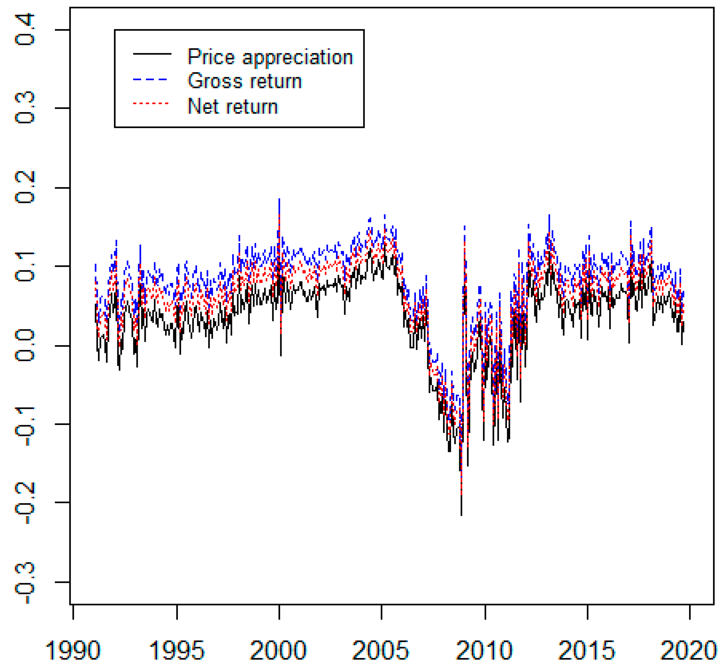
Figure 1 shows annualized house appreciation, gross and net returns for U.S. houses based on monthly data over 1991–2019. The gross return of houses is the sum of house appreciation and rent yield. House prices are from the FHFA index. Rent is the owner equivalent from the CPI. The dividend yield is the net of operating expenses, with rent and prices in currency. The return is the sum of house appreciation and the rent–price ratio net of expenses. The return begins to decline in 2005 before the 2008–2009 financial crisis. Real returns are negative throughout 2007–2013 and are accompanied with increased volatility.

Table 1. Summary Statistics.

Variable	Mean	Median	Minimum	Maximum	Standard Deviation
Price Appreciation	0.036	0.0469	−0.215	0.139	0.054
Gross Return	0.081	0.094	−0.172	0.186	0.054
Net Return	0.061	0.074	−0.190	0.166	0.054
Sales Turnover	0.192	0.192	0.082	0.286	0.048
Cross-Sectional Spread	0.020	0.016	0.000	0.089	0.021
Time-Frequency Volatility	0.013	0.000	0.000	0.074	0.018

has summary statistics. The mean rate of house inflation is 3.6% annually. The gross return, adding the rent–price ratio, is 8.1% and the net return is 6.1%. The average rate of inflation in the Consumer Price Index is 2.4%. Real appreciation has a mean of 1.2% annually. The gross and net real yields are 5.7% and 3.7%, respectively.

The standard deviation of the market return’s volatility is 5.4%. The idiosyncratic volatility is 2.0% and that for illiquidity is 1.3%. The volatility total is 8.7%. The real risk-adjusted return to a house is 3.7/8.7 or 0.42. S&P 500 has a mean real return of 8.2% with a standard deviation of 18.1%, for a Sharpe ratio with inflation as benchmark of 0.45. Houses and stocks have comparable risk-adjusted returns.

From Table 1, the cross-sectional idiosyncratic volatility averages 2.0% annually. The infrequent transaction volatility averages 1.3% annually. Adding market, idiosyncratic and illiquidity volatilities, a house has a standard deviation of 8.7% a year. The risk-adjusted return to a house becomes 3.7/8.7 or 0.42. In Giacoletti (2021), a house in California has a Sharpe ratio of 0.44 over a two-year holding period.

Over a comparable period, S&P 500 has an 8.2% mean real return with a standard deviation of 18.1%. The real risk-adjusted return on the S&P 500 is 0.45. Nasdaq 100 has a mean return of 15.03% with a standard deviation of 27.9%. The real risk-adjusted return is 12.63/27.9 and also 0.45.

A house has a risk-adjusted return comparable to either the S&P 500 or the Nasdaq 100. Houses have lower returns than the S&P 500. S&P 500 has a lower return than Nasdaq 100. Their risk-adjusted returns make houses comparable to these stock indices. All have risk-adjusted returns ranging between 0.42 and 0.45.

This is the standard deviation of the market return, suppressing idiosyncratic and infrequent transaction risks at 5.4% annually. Excluding cross-sectional and illiquidity volatilities, the risk-adjusted return to holding a house averages 3.7/5.4 or 0.69. With only market risk included, houses appear to have risk-adjusted returns that are 50% higher than stocks.

The 3.7% annually for a U.S. house’s real return compares with other estimates. Chambers et al. (2021) used portfolio holdings of four Oxford and Cambridge colleges. U.K. real house returns an average of 2.3% annually from 1901 to 1983. The long-run return to real estate over a century is 2.6% annually on U.K. and Singapore land leases (Giglio et al. 2021). Shorter-term real returns are 6% annually, with the yield curve negatively sloped.

Having rent and price appreciation, the rental yield, cross-sectional spreads, the inventory–sales ratio for volume and infrequent trading volatility as time series allows for due-diligence testing. Price appreciation, gross and net returns; the sales–inventory ratio; the cross-sectional spread; and volatility from infrequent reporting are stationary. These variables are appropriate for utilization in regressions.

Estimates on stationarity are shown in

Table 2. Stationarity.

Variable	Unit Root Test Statistics	Stationary
Price Appreciation	−0.202 *** (−5.009)	Yes
Gross Return	−0.201 *** (−4.660)	Yes
Net Return	−0.202 *** (−5.004)	Yes
Sales Turnover	−0.034 ** (−2.194)	Yes
Cross-Sectional Volatility	−0.119 *** (−4.389)	Yes
Infrequency Volatility	−0.149 *** (−5.003)	Yes

The table has the estimates of ${\alpha }_1$ with t-statistics in parentheses; *** significance at 1%; ** significance at 5%. Price appreciation, gross rand net returns, sales volume-to-listing ratio, cross-sectional spread and volatility from infrequent reporting are stationary.

with the augmented Dickey–Fuller unit root tests for stationarity. The null hypothesis of non-stationarity fails at 1%. The estimating equation for each variable is $\Delta y_t={\alpha }_0+{\alpha }_1{y}_{t-1}+{\sum }_{i=2}^{q+1}{\alpha }_i\Delta y_{t-i}+\nu$. The error is $\nu$; $\alpha$ are parameters; the variable being tested is $y_t.$ The null hypothesis is that ${\alpha }_1\ge 0$ and variable $y_t$ is nonstationary. The alternative is that ${\alpha }_1<0$ and $y_t$ is stationary. Lag order $q$ is based on the Akaike information criterion.

Expectations of appreciation and returns are best fitting from an autoregressive integrated moving average as an AR(6) process. The autocorrelation functions show gradual decay. The partial autocorrelation functions cut off at a lag of six months for all variables. The cutoff is consistent with using short-term expectations based on recent data.

Expectations are not based on a one-period lag alone. For house prices and expectations formation, the one-month lag weight is 0.222 (4.157). The two- and three-month lags are 0.144 (2.653) and 0.185 (3.389). The four-month lag is insignificant. The coefficients on five and six months move to 0.148 (2.724) and 0.127 (2.375) before losing significance. House dividend yield expectations have a similar pattern, falling in the first lagged quarter before a bounce in previous months five and six.

Table 3. Causality.

Appreciation
Variable	Not Causing	p-Value
Volume	Appreciation	0.000 ***
Appreciation	Volume	0.643
Cross-Sectional Volatility	Appreciation	0.000 ***
Appreciation	Cross-sectional Volatility	0.154
Infrequency Volatility	Appreciation	0.000 ***
Appreciation	Infrequency Volatility	0.201
Gross Return
Variable	Not Causing
Volume	Gross Return	0.000 ***
Gross Return	Volume	0.584
Cross-Sectional Volatility	Gross Return	0.000 ***
Gross Return	Cross-Sectional Volatility	0.167
Infrequency Volatility	Gross Return	0.000 ***
Gross Return	Infrequency Volatility	0.204
Net Return
Variable	Not Causing	p-Value
Volume	Net Return	0.000 ***
Net Return	Volume	0.625
Cross-Sectional Volatility	Net Return	0.000 ***
Net Return	Cross-Sectional Volatility	0.163
Infrequency Volatility	Net Return	0.000 ***
Net Return	Infrequency Volatility	0.203

*** significance at 1%.

shows Granger (1969) causality results between pairs from returns, on one hand, and volumes, cross-section and infrequency volatility on the other. In housing markets, causality runs from volumes and volatility to returns. Causality does not run from returns to volume. This conclusion applies in every paired case. All nine p-values in this direction are 0.000. Causality does not run from returns and appreciation to volumes and volatility. The lowest p-value is 0.163. The highest p-value is from appreciation and not the causing volume at 0.643. Causality results support returns, capital appreciation and yields being dependent. Volume and cross-sectional and infrequent trading volatility are causal.

These tests allow for the specification of the asset-pricing equation. Volume is causal to prices and on the right-hand side of estimation. Volume, appreciation and returns are stationary. With expectations controlled for, the asset-pricing equations for house appreciation and returns become estimated in volume. Volume factor estimation is in

Table 4. House asset pricing and volume.

Dependent	Price Appreciation		Gross Return		Net Return
	(1)	(2)	(3)	(4)	(5)	(6)
Intercept	−0.116 *** (−13.282)	−0.108 *** (−9.486)	−0.0760 *** (−8.850)	−0.067 *** (−6.044)	−0.093 *** (−10.800)	−0.085 *** (−7.555)
Volume	0.817 *** (18.592)	0.818 *** (18.350)	0.835 *** (19.374)	0.835 *** (19.125)	0.827 *** (19.070)	0.828 *** (18.822)
Adjusted R2	0.510	0.497	0.530	0.518	0.522	0.510
Monthly Fixed Effects	No	Yes	No	Yes	No	Yes
Months	331	331	331	331	331	331

Table 4 confirms that volume is a house pricing factor, exogenous and differing from financial markets. Estimates control for expectations. Volume is the sales–inventory ratio. Volumes lead and are positively correlated with prices, indicating liquidity. In financial markets, volume–return correlations indicate illiquidity. A 1% increase in volume from the sales–inventory ratio raises returns by between 0.817% and 0.835%. The volume pricing factor has t-statistics that are at least 18.59. Over the 30-year period, there are monthly dummies included to control for seasonal variation. The t-statistics are listed in parentheses. *** significant at 1%.

.

Table 4 confirms that a house has a unique volume–return relationship. In financial markets, illiquidity is when volumes affect returns, upwards or downwards. Liquid financial assets have no volume–return relationship. In Amihud (2002), the liquidity measure is the average of the absolute return divided by volume. A lack of liquidity is when volume moves absolute returns. This finding is reinforced by Amihud and Noh (2021).

In real estate, volume with liquidity raises returns (Krainer 2001). Lower volume and reduced liquidity reduce returns. With financial assets, liquidity has no impact on returns. Illiquidity changes returns upwards and downwards.

In Table 4 dependent variables include house appreciation and the gross and net returns. The net return is house inflation plus the after-expense rent income divided by the price. Volume is the sales–listing ratio. Estimates are after expectation controls.

The first two columns are for price appreciation. The columns exclude and include monthly fixed effects. Higher volumes increase returns. Lower volumes reduce appreciation and returns. A 1% increase in the sales–inventory ratio leads to a 0.818% increase in house appreciation. The gross return, including the rent–price ratio, increases by 0.835%. The net return increases by 0.828%. The range is tight between 0.817 and 0.835. The positive volume–return impacts are indicated by the t-statistics, with a minimum of 18.592.

Table 5. House asset pricing: volume and volatilities.

Dependent Variable	Price Appreciation		Gross Return		Net Return
	(1)	(2)	(3)	(4)	(5)	(6)
Intercept	−0.107 *** (−11.500)	−0.099 *** (−8.482)	−0.067 *** (−7.378)	−0.059 *** (−5.166)	−0.084 *** (−9.188)	−0.076 *** (−6.620)
Volume	0.778 *** (17.055)	0.779 *** (16.817)	0.798 *** (17.098)	0.799 *** (17.606)	0.789 *** (17.536)	0.790 *** (17.295)
Infrequency Volatility (Monthly/Quarterly)	0.091 *** (3.327)	0.085 *** (3.281)	0.042 *** (3.098)	0.035 *** (3.057)	0.063 *** (3.208)	0.056 *** (3.164)
Idiosyncratic Volatility	0.690 *** (2.611)	0.699 *** (2.593)	0.663 *** (2.546)	0.672 *** (2.529)	0.676 ** (2.583)	0.685 ** (2.566)
Adjusted R2	0.519	0.505	0.538	0.525	0.531	0.518
Month Fixed Effects	No	Yes	No	Yes	No	Yes
Observations	331	331	331	331	331	331

Volume is the sales–inventory ratio. t-statistics are in parentheses. *** significant at 1%; ** significant at 5% level. Dependent are returns for house inflation and the gross and net return. Causal variables are volumes, the idiosyncratic and infrequent transaction volatilities. Over the 30-year period, there are monthly dummies included to control for seasonal variations.

shows house asset pricing in causal volume and volatility. Volatility is cross-sectional and for infrequent transactions as the monthly–quarterly ratio. Variables are stationary and the causal direction from volume and volatility to prices and returns has been established.

House appreciation and returns have been shown to be caused by volume and volatility. With these variables on the right-hand side, returns increase in volume and volatility. Expectations have been adjusted for. House appreciation and the gross and net return are dependent. Causal variables are volumes, the idiosyncratic and infrequent transaction volatilities.

House appreciation and returns are increasing in volume with volatility included. The range for a 1% increase in the sales–inventory ratio is for appreciation and returns to increase by between 0.778% and 0.790%. The volume–return positive correlation remains as a different liquidity effect for houses compared with stocks. Conversely, a 1% decrease in sales relative to inventory reduces the net return by between 0.789% and 0.790%. The t-statistics are between 16.82 and 17.61.

Liquidity drive houses volumes and prices higher together. The positive liquidity from volume continues with the volatility included. A 1% increase in the sales–listing ratio leads house prices to increase by 0.779% with monthly fixed effects. Liquidity raises house returns in volume. A financial asset that returns responsiveness to volume indicates illiquidity.

Estimation is with quarterly volatility as the cross-section idiosyncratic risk measure. A 1% increase in cross-sectional volatility leads to a housing price appreciation that is between 0.69% and 0.70% depending on whether monthly fixed effects are included or not. Gross returns increase by between 0.663% and 0.672% for a 1% increase in idiosyncratic risk. Net returns after expenses increase by 0.676% to 0.685%.

A 1% increase in infrequency volatility increases house appreciation and returns by between 0.035% and 0.091%. The associated t-statistics are between 3.057 and 3.327. Idiosyncratic or volatility leads to an increase in returns across the six specifications.

Infrequency volatility in the ratio of monthly to quarterly volatility increases returns in all specifications. The range is between 3.5 and 9.1 basis points in higher returns for a one percentage point increase in relative volatility.

Each factor contributes to liquidity or its absence. The impact of volumes on prices is a liquidity risk. Liquidity from transaction infrequency confirms higher volatility at shorter time periods (Giacoletti 2021; Sagi 2021). Housing returns increase when transactions are more infrequent and consistent. Switching from monthly to quarterly data reduces the standard deviation of reported house price appreciation by smoothing.

6. Conclusions

There are idiosyncratic and illiquidity risks from investing in housing. Idiosyncratic risks are from similar houses selling for different prices at the same time. Autocovariances in rents and prices create bid–ask spreads and cross-sectional distributions. These distributions measure the idiosyncratic risk.

Illiquidity risks are from the variance ratios of monthly and quarterly rent and price distributions. These ratios derive estimates of the unobserved daily volatility smoothed out in suppressing illiquidity.

House data are reported at low frequency, usually in monthly and in index form. Taking the standard deviation of these measures understates the risk of holding a house. For monthly data three decades since 1990, the average annual return net of a risk-free rate is 3.7% annually. The standard deviation of this return is 5.4%. The resultant Sharpe ratio is 0.69. The comparable Sharpe ratio for the S&P 500 stock index is 0.42.

A house earns a risk-adjusted return that is 64% higher than on a stock index. This occurs despite houses having lower measured risk. Houses are off the frontier of a risk-return tradeoff, earning returns with minimal measured risks.

Another risk is illiquidity from infrequent transactions in houses. The bid–ask spreads in house prices and rents are reconstructed for quarterly data. The outcome is the standard deviation of the quarterly return. The monthly–quarterly volatility ratio measures the smoothing from infrequent data reporting. The ratio derives an implied volatility for daily house returns. This illiquidity volatility has been smoothed out by monthly reporting.

The house price and rent bid–ask spreads are constructed on the FHFA-BLS data set and sample period. The resulting idiosyncratic risk from cross-section volatility adds 2.0% to the return standard deviation. The implied illiquidity volatility adds another 1.3% annually. The mean excess return is unchanged at 3.7% annually. The annual standard deviation of the return becomes 8.7%. The Sharpe ratio of a house is 0.43. This estimate is comparable to that for stocks.

Houses sell and rent for different prices at the same time. This behavior leads to a bid–ask spread in prices and rents. The return to a house is the sum of price appreciation and a net rent–price ratio. A spread in rents and prices affects returns from this cross-sectional idiosyncratic risk.

Data on houses are consequently reported less frequently, such as monthly than for financial markets. Financial market data are continuous during trading and are reported daily at a minimum. The resulting data smooth the illiquidity from infrequent sales.

Out of necessity, house returns must use these monthly data on prices and rents. However, as a measure of risk, the standard deviation of the overall monthly return suppresses the bid–ask spreads that participants face. The volatilities from idiosyncratic and illiquidity risks are removed. This volatility suppression makes houses appear to have higher and even implausible risk-adjusted returns.

A caveat is that all conditions of financial markets do not translate immediately to real estate. Real estate trades infrequently and after negotiation. The return to real estate ties to volume, but it is different from that in financial markets. In Amihud (2002) and Amihud and Noh (2021) illiquidity earns a return. Illiquidity is the absolute return divided by volume. Trading volume moves returns up or down for illiquid stocks. In real estate, liquidity in volume moves returns upwards. Low volume moves returns downwards. Returns, and not their absolute value, are correlated with volume.

Another caveat is while the sample has provided the reported results, it would be appropriate to test other markets. It remains the case that, at the aggregate level, housing data for prices and rents are reported as a single index. The procedures here offer a method for addressing these index data reported as single numbers.

Information on houses is likely to continue to be reported in index numbers and at low monthly frequencies. Interpreting the data and constructing risk-adjusted returns require taking an account of the distributions of prices and rents that households face. Otherwise, houses appear to offer returns with minimal risk.