COVID-19 Mortality and Economic Losses: The Role of Policies and Structural Conditions

Abstract

The response of governments to the COVID-19 outbreak was foremost oriented to two objectives: saving lives and limiting economic losses. However, the effectiveness and success factors of interventions were unknown ex-ante. This study aims to shed light on the drivers of countries’ performances during the first year of the COVID-19 pandemic. We measure performances by excess mortality and GDP growth adjusted for additional fiscal stimulus. We conduct an empirical analysis in two stages: first, using hierarchical clustering, we partition countries based on their similarity in health and economic outcomes. Second, we identify the key drivers of outcomes in each country cluster by regression analysis, which include linear, least absolute shrinkage and selection operator (LASSO), and logit models. We argue that differences in countries’ performances can be traced back both to policy responses to COVID-19 and structural conditions, the latter being immutable over the pandemic. Three relevant structural conditions emerge from the results: trade reliance on services, corruption, and the size of the vulnerable population (elderly, low-income, smoking, or cardiovascular-failing). Policies such as large-scale open public testing and additional fiscal stimulus in non-health could help reduce excess mortality, which might lead to lower economic losses.

1. Introduction

During the first twelve months of the COVID-19 pandemic, countries around the world seemed to choose between two different approaches: saving lives by locking down their economies or saving their economies by trying to mitigate the health impact of contagion. The first approach, sometimes referred to as zero-COVID or elimination strategy, aims at eradicating the virus from a country. Its proponents claim that the economic costs associated with strict containment measures and quicker elimination of the virus are lower compared to the prolonged costs deriving from mitigation strategies (König and Winkler 2021; Oliu-Barton et al. 2021). The second approach, called mitigation strategy, or living with COVID19, rests on the idea that the virus cannot be eliminated (Phillips 2021), but the impact of contagion can be mitigated by pharmaceutical intervention to flatten the curve while keeping a certain degree of openness and freedom of movement. Advantages include better social and economic sustainability in the long run. The review of the benefits and drawbacks of both strategies in the later months has driven the search for alternative policies which might save lives without creating excessive economic losses (Daumann et al. 2021; Rampini 2020), with some countries changing their strategy (Blair et al. 2022). However, irrespective of the beliefs about what approach best suits a country, the effectiveness and success factors of governments’ interventions were unknown ex-ante and country specific.

This paper addresses the factors that explain the success or failure of governments in counteracting the health and economic effects of COVID-19. We argue that the outcomes of strategies may be contingent on preexisting “structural” conditions to a certain extent, such as countries’ demographic, geographic, economic, and public health characteristics, which are hardly adjustable in the short run. These conditions combine with non-pharmaceutical and fiscal policies into country-specific outcomes. In other words, success might be altered by factors that are not in the control of policymakers, despite their plans. In view of this, the literature began to recognize the need to identify structural drivers affecting policy designs and pandemic performance (Bourdin et al. 2022; Islam et al. 2020).

We seek to answer two fundamental research questions: How did countries perform, one year after the outbreak, judged jointly by health and economic outcomes? What are the potential drivers of their performances in terms of structural conditions and policy responses? To answer the first question, we assess countries’ results up to one year after the World Health Organization (WHO) declared the COVID-19 outbreak. More precisely, the assessment relies on health and economic outcomes measured through excess mortality and economic losses,1 respectively, up to 31 March 2021. Specifically, we choose excess COVID-19 mortality and economic losses because we believe they are the most representative variables on the two ends of the policy trade-off: one reflecting the cost paid in terms of human lives, the other the cost borne by the economy. From the indicators for human and economic losses, countries are partitioned into groups by agglomerative hierarchical clustering based on similarity along the two dimensions. To answer the second research question, we conduct an econometric analysis to find structural conditions or policy measures that might have increased the probability of a country being assigned to each group. We employ linear, least absolute shrinkage and selection operator (LASSO), and logit models.

We found that, while countries that have pursued elimination strategies (mainly the green group) were successful in containing mortality but showed high economic losses due to huge fiscal stimuli, the performances of countries that have implemented mitigation strategies are scattered. One group (blue) could contain both COVID-19 excess mortality and economic losses, which makes it the most successful in our study. A second one (purple) kept economic losses under control at the price of the highest mortality rate. Another (gray) shows high economic losses with an intermediate mortality rate. All the remaining groups stand in between those four. Furthermore, we did not find a clear trade-off between saving lives and saving the economy judged by health and economic outcomes (see Alvarez et al. 2021). Above all, the position of countries in the bi-dimensional plane does not always reflect their initial strategies. Thus, why do countries following similar strategies show different performances? In addition, if achieving low economic losses and mortality was feasible, why could only some countries succeed? We argue that it is due to the heterogeneity in policy implementations and structural characteristics. Countries that achieved an excellent performance might have benefited from either favorable structural conditions, effective policies, or both. We found novel attributes explaining countries’ health and economic outcomes. Structural variables such as trade reliance on services and corruption might change the incentives of individuals and policymakers in terms of policy compliance and implementation, respectively. Policies such as large-scale open public testing and additional fiscal stimulus in non-health could help reduce excess mortality through different channels, leading to lower economic losses.

The results contribute to an emerging body of literature attempting to find what structural conditions, understood as conditions that cannot be changed within a short-time window, and policies are the most relevant in the fight against COVID-19 and ultimately affect countries’ performances judged by health and economic outcomes. Although some of the attributes we include in the analysis are already employed in other works, our study advances researchers’ understanding about what are the most relevant factors for explaining a country’s position in the human-economic losses space. In other words, we attempt to uncover what factors are associated with each country cluster, which reflects different degrees of success in dealing with the pandemic. Moreover, the research design is original. Specifically, how we conduct the empirical strategy by combining clustering with econometric analysis is an element of novelty.

The remainder of the paper is organized as follows: Section 2 provides a summary of related literature and identifies the research gap. Section 3 presents data and methodology, while Section 4 discusses our results. Section 5 discusses policy recommendations and limitations. Section 6 presents conclusions.

2. Related Literature

This paper is part of emerging literature that seeks to identify countries’ structural characteristics and policies that connect with the success in dealing with the COVID-19 pandemic.

The papers of Brodeur et al. (2021, 2022) focus on structural characteristics and non-pharmaceutical policies, respectively. Analogous to our approach, Bourdin et al. (2022) draw attention to what we defined as countries’ structural characteristics. The heterogeneous impact of the pandemic in Europe is better understood by looking at regional attributes. These are classified into two categories: socioeconomic and pandemic-related attributes. Desirable socioeconomic factors reduce vulnerability and set a solid foundation for disease management. On the other hand, pandemic-related variables such as the number of hospital beds influence exposure to the virus. Through these channels, structural conditions ultimately determine the health outcomes of countries. Brodeur et al. (2021) present a comprehensive literature survey focusing on the determinants, effectiveness, and compliance of social-distancing policies. The study also gathered literature on various socioeconomic consequences of COVID-19 in terms of labor, health, gender, discrimination, and the environment, among others.

Another early body of work focused on the effectiveness of COVID-19 policies in minimizing the health costs. For instance, using a difference-in-differences methodology, Fang et al. (2020) argue that lockdowns in Wuhan during January 2020 prevented a 105% increase in COVID-19 cases in Chinese cities outside of the Hubei Provence. In turn, Friedson et al. (2020) used a synthetic control research design to estimate that shelter-in-place orders reduced COVID-19 cases by 125.5 to 219.7 per 100,000 population and prevented 1661 deaths during its first month of application. Haug et al. (2020) use variable selection techniques, such as the least absolute shrinkage and selection operator (LASSO), to identify effective policies that reduce the reproduction number of COVID-19. They find that the effectiveness of non-pharmaceutical interventions on health outcomes depends on country-specific factors.

Others have studied the impact of policies on economic activity during the pandemic. Sheridan et al. (2020) compare real-time transaction data between Denmark and Sweden to argue that aggregate spending dropped mainly due to the virus and not to policies that restricted social and economic activities. Consistently, Maloney and Taskin (2020) show that, for the United States, the decrease in mobility is voluntary and not the result of social distancing policies. As a result, these authors find that the impact of the virus on economic activity, measured as restaurant reservations and movie spending, is due to voluntary individual decisions and not government policies. The paper of Boitan et al. (2021) seeks to investigate whether health-related variables have shaped the economic sentiment of European countries during the pandemic. Similarly to our approach, they use hierarchical clustering to group European countries based on five sentiment indicators. Next, they conduct five-panel regression analyses, where COVID-related health variables are regressed on the five sentiment indicators separately. Unlike our study, the results from the clustering are not part of the regression.

Finally, a part of the literature deals with the health and economic costs of COVID-19 strategies and interventions. As argued by Miguel and Mobarak (2021), the earliest contributions modeled optimal targeted policies such as lockdowns for the old could reduce health and economic costs (Acemoglu et al. 2021). Barbieri Góes and Gallo (2021) show that, in the absence of COVID-19 elimination strategies, pandemic-driven recessions might emerge. Similar results are obtained by Delli Gatti and Reissl (2022), who, by comparing alternative epidemic scenarios using a macro-epidemiological agent-based model, find that the trade-off between lives and livelihood is remarkable in the early stage of the lockdown but fades away in the long run. Empirical studies such as Arias et al. (2021), Kochańczyk and Lipniacki (2021), and Oliu-Barton et al. (2021) confirmed the positive roles of policies in shaping better health and economic outcomes.

To the best of our knowledge, no studies seek to identify what structural conditions and policies affect health and economic outcomes simultaneously. However, we share a similar setting with the paper of Alvelda et al. (2020) as they classify countries’ performance in “Economic Loss versus the Loss of Lives”. Alvelda et al. (2020) argue that to save the economy policymakers should implement measures that focus on minimizing the number of deaths. To do so, the authors suggest that governments should use abatement and subsidies geographically targeted by data on COVID-19 prevalence.

3. Materials and Methods

In this section, we describe the methodologies and data that are employed to investigate the research questions. In a nutshell, our approach breaks down into four steps:

• We set up the problem in terms of the fundamental trade-off we intend to study: human versus economic losses. The construction of these two key variables is detailed in Section 3.1;
• We identify relevant variables for the study and collect them into a data set from a variety of sources (Section 3.2);
• Given the performances of countries in terms of economic and human losses built in Section 3.3, we conduct a clustering analysis that aims to partition countries into groups more or less successful along the two dimensions;
• From the six-country clusters arising from clustering, we use econometrics to estimate what are the most relevant factors that affect the probability of a country being included in each group (Section 3.4).

3.1. Economic and Human Losses

3.1.1. Economic Losses

To evaluate the broad impact of the pandemic on the economy, we construct an indicator $\mathcal{L}$ for economic losses. These are defined as the changes in real GDP net of additional fiscal expenditure before and after the outbreak. The quarterly GDP data are from the OECD National Accounts following expenditure approach (CQR: National currency, current prices, quarterly levels);2 additional fiscal stimulus “above-the-line” from January 2020 to March 2021 data were collected by the IMF Fiscal Affairs Department through the Fiscal Monitor Database of Country Fiscal Measures in Response to the COVID-19 Pandemic (IMF 2021).

Building on GDP is a convenient way to account for economic losses during the pandemic (Boitan et al. 2021; Ludvigson et al. 2020), as GDP is a comprehensive indicator for economic activity; it is readily available for many countries at monthly or quarterly frequency; based on the definition of GDP, losses could be interpreted as a drop in either the total added value, or the aggregate expenditure, or the aggregate income.

One would be tempted to compute the loss in GDP as the difference from a reference period in the past. Even if such an approach is logically correct, the resulting indicator would be biased by the additional fiscal expenditure put in place by governments to contrast both falls in GDP and the health emergency. For instance, suppose that countries A and B, starting from identical initial conditions, showed the same decline in GDP after a shock but country A put in place an expansionary fiscal policy financed by debt while country B did not. Then, solely observing the change in GDP would lead us to conclude that both countries had the same losses. However, the fiscal expenditure operated by A supported the economic activity after the shock, thus preventing a further decline in GDP. In other words, we would not think of the positive impact of fiscal expenditure on the GDP of country A. However, to achieve the same outcome, country A employed more resources than B.

Our definition of economic losses incorporates the argument outlined in the example above. Let us consider the GDP by the expenditure approach, $GDP=C+I+G+NX$, i.e., the gross domestic product is the sum of aggregate consumption, investment, government spending, and net exports. Since the outstanding variation in G over the outbreak, the change in GDP by itself hides the additional costs borne by the government. Therefore, to calculate economic losses, we amend the change in GDP for additional fiscal spending. In other words, GDP at the time t is decreased by additional spending to filter the extraordinary fiscal expansion during the pandemic.3 Moreover, surging inflation rates observed for some countries affected nominal variables. To avoid economic losses being shrunk, we correct for the inflation rate between $t-1$ and t. Economic losses are defined

$${\mathcal{L}}_t:=-\left(\frac{GD{P}_t-G_t^{add}}{(1+{\Pi }_t)GD{P}_{t-1}}-1\right)$$

(1)

where $GD{P}_t$ is the nominal GDP between 2020-Q1 and 2021-Q1; $GD{P}_{t-1}$ is the nominal GDP for all quarters of 2019 plus 2019-Q14; ${\Pi }_t$ is the inflation rate computed as the year-on-year change in the consumer price index between 2019 and 2020; $G_t^{add}$ is nominal discretionary additional “above-the-line” fiscal expenditure that supplements automatic stabilizers.

There are two further reasons for including additional spending in the losses bill. First, some spending was triggered by panic following past policy failures. Lengthy panic spending should be avoided, as it is merely a remedy for poor policy design in the past. Second, additional fiscal spending adds pressure to the national debt: it increases repayments for future households, makes debt financing costlier, and leads to potential default. Future research could distinguish effective from ineffective spending, which generates undesirable economic losses and has no significant return in saving lives.

3.1.2. COVID-19 Excess Mortality

The second key variable representing human losses is COVID-19 excess mortality, defined as the increase in all-cause mortality after the outbreak over the expected baseline mortality supported by historical trends (Karlinsky and Kobak 2021).

To calculate excess mortality, we closely follow the approach of Karlinsky and Kobak (2021). First, baseline mortality for 2020 is predicted at the country level through a linear regression model with time-fixed effects on the intercepts using data from 2015 to 2019. Second, excess mortality is defined as the difference between the all-cause observed death numbers and baseline mortality. Lastly, we sum over the quarterly differences ranging from 2020-Q1 to 2021-Q1, divide by the country population, and multiply by one million. We obtain a measure of excess COVID-19 mortality per million people at 2021-Q1.

Excess mortality during the pandemic can be roughly decomposed (see Karlinsky and Kobak 2021, p. 10) in:

$$\begin{array}{cc}\hfill \mathrm{excess}\mathrm{mortality}& =\left(\mathrm{A}\right)\mathrm{deaths}\mathrm{directly}\mathrm{caused}\mathrm{by}\mathrm{COVID-19}\hfill \\ \hfill & +\left(\mathrm{B}\right)\mathrm{deaths}\mathrm{caused}\mathrm{by}\mathrm{medical}\mathrm{system}\mathrm{overload}\mathrm{during}\mathrm{COVID-19}\hfill \\ \hfill & +\left(\mathrm{C}\right)\mathrm{excess}\mathrm{deaths}\mathrm{from}\mathrm{other}\mathrm{causes}.\hfill \end{array}$$

The largest number of deaths comes from (A) and (B), where (B) follows from contagion waves for which the health system was unprepared. (C) encloses several elements: natural and unnatural causes of death plus extreme events like wars5 or natural disasters. For most countries, (C) is negative and reflects the lives indirectly saved by COVID-19 restrictions, e.g., reduction in the mortality from seasonal influenza or traffic incident fatalities following social distancing and mobility reduction.6 For some countries in our sample (e.g., New Zealand, Malaysia, Uruguay), the effect of (C) exceeds (A)+(B), resulting in negative excess mortality. Although counter-intuitive, for these countries, health policies prevented the mortality rate from exceeding its baseline value. The fact is observed in the time range of our analysis and holds under the applied methodology, so we cannot exclude it may change on a longer interval or under another approach to estimate excess mortality.

An alternative measure of human losses is reported COVID-19 deaths per million. Compared to excess mortality, it does not require to be estimated as it simply builds on the aggregation of all COVID-19 deaths reported in a country. As such, it does not suffer from statistical biases. In addition, it measures exactly COVID-19 mortality. However, the reporting protocols are not standardized resulting in cross-country inconsistencies in reported deaths caused by COVID-19.7 Furthermore, some countries, e.g., Romania and Russia, severely under-reported the number of deaths in official statistics.8 In light of this, we prefer to measure human losses in terms of excess mortality as it is a more objective indicator: first, it avoids reporting inconsistencies by applying the same estimation methodology to all countries. Second, it filters the impact of country-specific health characteristics on mortality by accounting for the baseline mortality rate, thus limiting the effects of confounding factors on the assessment of COVID-19 mortality.

3.2. Structural Conditions and Policy Variables

In this section, we explain the choices of structural conditions and policy variables and detail data sources.

Our structural conditions include health, demographic, geographic, and economic characteristics. The first health attribute we choose is past pandemic experience. As argued in Basher and Haque (2021), the lessons of the SARS pandemic might have helped contain the virus in East Asian countries. Therefore, we include SARS cases and H1N1 death as proxies for the past pandemic experience (ECDC 2010; WHO 2015). Other variables reflecting public health (see Bourdin et al. 2022) are share of population above 70 (Our World in Data 2022c), hospital beds (The World Bank 2022a). The share of population above 70 is selected as the elderly population might be most vulnerable to COVID-19. Hospital beds capture the development of the healthcare sector and supply of health services. To further capture the supply health services, we include the variable doctor (The World Bank 2022b), which measures the number of physicians per thousand people. To control the health status of the population, we include cardiovascular death rate (Our World in Data 2022a), diabetes prevalence (Our World in Data 2022b) and smoking prevalence (The World Bank 2022d). Studies such as Bourdin et al. (2022), Clift et al. (2022) and Sanchez-Ramirez and Mackey (2020) argues that these variables could potentially influence the stringency index or health outcomes such as the COVID-19 deaths. We add neighboring countries (Geodatasource 2022) and population density (The World Bank 2022c) to the list of regressors to control if the number of borders and the population concentration have an effect in easing contagion.

Structural characteristics mostly related to the economy are the Gini index, the trade reliance on goods or services, and the degree of digitalization of the economy. Wildman (2021) suggests that income inequality captured by Gini (OECD 2022) coefficients might be associated with poor health outcomes during the pandemic. Trade reliance on goods or services (The World Bank 2022e, 2022f) captures countries’ import and export volume as a percentage of GDP prior to the pandemic. Trade might affect the health and economic outcomes of countries through various channels, for which the reader is referred to Section 4. Dingel and Neiman (2020) estimated the share of jobs that can be done at home before 2020. In light of the research, we constructed the variable digitalization. Surprisingly, digitalization is highly correlated with trade reliance on services: since many jobs in the tertiary sector can be operated from home, many countries with an advanced service sector also rely heavily on the trade of the services produced.

We draw pandemic-related policy measures from the Oxford COVID-19 Government Response Tracker (Hale et al. 2021). It covers a wide range of health policy responses for different countries. Although there are competing data sources on the national level, this data set is the most suitable for our cross-country study. Each policy variable records the daily average level of policy announcements from January 2020 to March 2021. In Hale et al. (2021), efforts have been made to record policies that have been effectively implemented. However, a gap might still exist between actual policy implementations and government announcements. Therefore, we control for the corruption level by country using the corruption perception index (Transparency International 2022). Initially, our study used democratic ratings to control for the heterogeneity between the governments. However, such a proxy variable is not optimal as countries such as Singapore have low democratic ratings, but their governments are transparent and not so corrupted.

The economic policy measures we consider are additional fiscal stimulus in health and non-health, government debt, and tax revenue. The additional fiscal stimulus in health and non-health (IMF 2021) captures fiscal policy during the pandemic, which might impact the health and economic outcomes of countries. We explicitly exclude conventional monetary policy. In general, monetary policy is ineffective close to the zero lower bound. Furthermore, Long et al. (2022) suggests monetary policies had a positive effect in controlling inflation, but the impact on reducing the unemployment rate is minimal. The national debt level and tax revenue might influence the conduct of fiscal policy and eventually the economic performance of countries.

The time range of the analysis is between the beginning of 2020 and 31 March 2021, covering approximately from when the WHO recognized COVID-19 as a Public Health Emergency of International Concern to the phasing-in of the vaccination campaign in several countries. The time range is chosen to evaluate countries’ performance as a result of policies and structural conditions. Including the following quarters would result in capturing countries’ differences connected to the effectiveness of vaccines, which is not investigated in this study.

Furthermore, the sample selection is conditioned by cross-country data availability. The clustering analysis is carried out for 55 countries in the selected date range.9 We excluded Azerbaijan, Belarus, Ukraine, and Egypt from the sample due to unreliable reported economic data which would lead to a severe underestimation of economic losses. As data on health policies and structural conditions are not available for all countries, the sample reduces to 46 countries.10 

Table 1. Descriptive statistics.

	Mean	SD	Min	Max
Outcome Variables
Excess mortality	1120.67	1095.57	−409.30	3441.87
Economic losses	−8.92	4.96	−21.90	0.52
Structural Conditions
H1N1 death	269.74	601.30	2.00	3433.00
SARS cases	12.70	50.21	0.00	251.00
Tax Revenue	20.00	5.99	9.78	34.28
Population density	4.35	1.44	1.16	8.98
Share of population above 70	10.49	3.84	2.66	18.49
Gini	35.27	7.98	24.20	65.00
Smoking prevalence	24.98	7.52	7.90	44.70
Doctors	3.29	1.17	0.60	6.35
Cardiovascular death	180.60	97.79	79.37	431.30
Diabetes prevalence	6.78	2.54	3.28	16.74
Hospital beds	4.39	2.66	1.00	13.05
Trade reliance on services	32.77	46.87	5.54	295.80
Trade reliance on goods	72.23	39.03	19.45	209.90
Corruption	62.70	17.67	28.00	87.00
Neighboring countries	3.70	2.99	0.00	14.00
Government debt	65.09	43.11	8.44	234.86
Digitalization	34.64	8.40	15.02	58.07
Schooling	11.56	1.65	7.20	14.10
Policy Variables
School closures	54.34	14.18	17.00	80.25
Workplace closing	48.92	12.36	13.50	67.52
Cancel public events	67.43	12.70	25.22	87.61
Restrictions on gatherings	64.38	13.70	2.99	84.71
Close public transport	20.15	15.53	0.00	52.81
Stay at home order	30.05	12.67	0.00	65.81
Internal movement restrictions	37.97	19.54	0.00	64.29
International travel restrictions	64.23	12.50	34.93	90.40
Public information campaigns	88.76	6.80	54.24	99.78
Testing policy	61.37	14.97	26.19	93.01
Manual contact tracing	69.73	17.85	26.12	100.00
Facial coverings	44.33	16.58	5.39	77.40
Protection of elderly people	55.13	18.87	7.59	84.26
Fiscal stimulus in health	1.10	1.18	0.03	7.52
Fiscal stimulus in non-health	6.81	4.71	0.21	22.15
Observations	46

reports the descriptive statistics for outcome, structural-condition and policy variables. Detailed descriptions of each variable are presented in

Table A1. Variable descriptions: structural conditions.

Variable	Description
H1N1 death	Cumulative number of H1N1 deaths
SARS cases	Cumulative number of SARS cases includes number of deaths
Share of population above 70	Share of the population that is 70 years and older in 2015
Cardiovascular death	The annual number of deaths from cardiovascular diseases per 100,000 people in 2017
Diabetes prevalence	Percentage of people ages 20–79 who have type 1 or type 2 diabetes in 2017
Smoking prevalence	Prevalence of current tobacco use as a percentage of adults in 2018
Hospital beds	Hospital beds per thousand people, most recent year available before 2021
Doctors	Physicians per 1000 people, most recent year available before 2021
Neighboring countries	Number of countries bordering
Population density	Log number of people divided by land area measured in square kilometers, most recent year available since 2018
Gini	Gini coefficient in 2019
Schooling	Average number of years of total schooling across all education levels for the population aged 25 and above, most recent year available before 2020
Corruption	Corruption perception index in 2019
Trade reliance on services	Imports and exports of services as a percentage of GDP, most recent year available prior to 2020
Trade reliance on goods	Imports and exports of goods as a percentage of GDP, most recent year available prior to 2020
Digitalization	Estimated share of job that can be done at home before 2020
Government debt	General Government Gross Debt as a percentage of GDP in 2019
Tax Revenue	Tax revenue as a percentage of GDP in 2019

and

Table A2. Variable descriptions: policy measures.

Variable	Description
School closures	Daily average level from January 2020 to March 2021, normalized to 100. 0—No measures, 1—Recommend closing or all schools open, 2—Require partial closing, 3—Require closing all levels.
Workplace closing	Daily average level from January 2020 to March 2021, normalized to 100. 0—No measures, 1—Recommend closing, 2—Require closing for some sectors or categories of workers, 3—Require closing for all-but-essential workplaces.
Cancel public events	Daily average level from January 2020 to March 2021, normalized to 100. 0—No measures, 1—Recommend cancelling, 2—Require cancelling.
Restrictions on gatherings	Daily average level from January 2020 to March 2021, normalized to 100. 0—No restrictions, 1—Restrictions on very large gatherings above 1000 people, 2—Restrictions on gatherings between 101–1000 people, 3—Restrictions on gatherings between 11–100 people, 4—Restrictions on gatherings of 10 people or less.
Close public transport	Daily average level from January 2020 to March 2021, normalized to 100. 0—No measures, 1—Recommend closing, 2—Require closing.
Stay at home order	Daily average level from January 2020 to March 2021, normalized to 100. 1—Recommend not leaving house, 2—Require not leaving house with exceptions for daily exercise, grocery shopping, and essential trips, 3—Require not leaving house with minimal exceptions.
Internal movement restrictions	Daily average level from January 2020 to March 2021, normalized to 100. 0—No measures, 1—Recommend not to travel between regions or cities, 2—Internal movement restrictions in place.
International travel restrictions	Daily average level from January 2020 to March 2021, normalized to 100. 0—No restrictions, 1—Screening arrivals, 2—Quarantine arrivals from some or all regions, 3—Ban arrivals from some regions, 4—Ban on all regions or total border closure.
Public information campaigns	Daily average level from January 2020 to March 2021, normalized to 100. 0—No COVID-19 public information campaign, 1—Public officials urging caution about COVID-19, 2—Coordinate public information campaign across traditional and social media.
Testing policy	Daily average level from January 2020 to March 2021, normalized to 100. 0—No testing policy, 1—Only those who both have symptoms and meet specific criteria such as being key workers, 2—Testing of anyone showing COVID-19 symptoms, 3—Open public testing such as drive through testing available to asymptomatic people.
Manual contact tracing	Daily average level from January 2020 to March 2021, normalized to 100. 0—No contact tracing, 1—Limit contact tracing which is not done for all cases, 2—Comprehensive contact tracing done for all identified cases.
Facial coverings	Daily average level from January 2020 to March 2021, normalized to 100. 0—No policy, 1—Recommend, 2—Require in some specified public spaces, 3—Require in all public spaces with other people present, 4—Require in all public spaces at all time.
Protection of elderly people	Daily average level from January 2020 to March 2021, normalized to 100. 0—No measures, 1—Recommend isolation, hygiene, and visitor restriction measures in long term care facilities or recommend elderly people to stay at home, 2—Narrow restrictions for isolation, hygiene in long term care facilities and some limitations on external visitors, recommend restrictions protecting elderly people at home, 3—Extensive restrictions for isolation and hygiene in long term care facilities, all non-essential external visitors prohibited. All elderly people required to stay at home, not leave the home with minimal exceptions and receive no external visitors.
Fiscal stimulus in health	Additional fiscal spending above the lines in health as a percentage of GDP, from January 2020 to March 2021.
Fiscal stimulus in non-health	Additional fiscal spending above the lines in non-health sectors as a percentage of GDP, from January 2020 to March 2021.

.

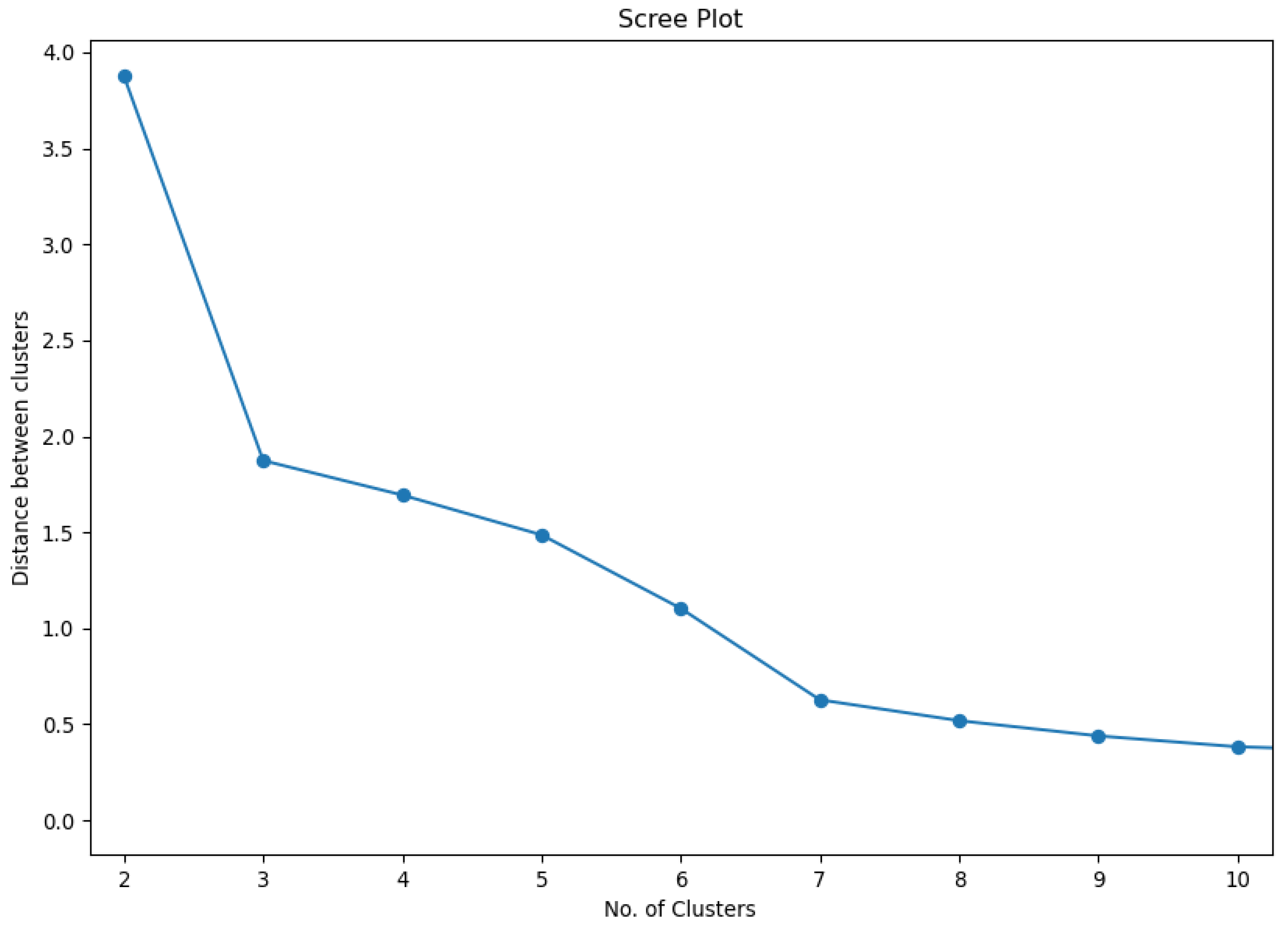
3.3. Hierarchical Clustering

Cluster analysis, or data clustering, is a way of partitioning observations in a dataset based on their similarity. The diffusion of cluster analysis has burst in the last years due to its abundant application to big data. Despite it being initially developed in statistics and computer science, cluster analysis is established in many disciplines, among which economics and finance. A comprehensive treatise on the subject including Matlab and C++ code examples can be found in Gan et al. (2020).

We employ a clustering algorithm for grouping countries before conducting a more sophisticated quantitative analysis. The basic principle is to form partitions such that intra-group observations are as similar as possible, and groups are as different as possible. There are different types of algorithms depending on how observations are clustered together (hierarchical clustering, k-means, DBSCAN, etc.). In what follows, we employ a hierarchical agglomerative clustering algorithm (see Murtagh and Contreras 2017) (HAC henceforth). HAC is a model-free algorithm, i.e., it groups data points regardless of any prior assumptions about the data-generating process. Moreover, we prefer it to alternatives because of the transparency of the algorithm, a simple and intuitive interpretation from the dendrogram, and an arbitrarily defined number of clusters. Shortcomings are the sensitivity to noise and outliers, and, being theory-free, some degree of arbitrariness in its implementation.

In HAC, objects are connected from the bottom-up depending on how similar they are to each other. HAC constructs a binary tree starting from single objects (leaves) to the root. The smallest clusters are made of one object. At each step, the two closest clusters are merged into another one so that larger clusters are formed by agglomerating the closest objects based on selected measures. The process is iterated until all objects are grouped into a single cluster. The graphical representation of the tree is called a dendrogram.

Clusters are formed by moving from leaves to the root of the dendrogram. However, clustering trees might look different even for the same sets of observations and features depending on base distance and the linkage functions. The former measures the distance between any two elements in the sample. Distances describe the degree of similarity between observations. At the first stage of the clustering algorithm, two leaves are merged into one cluster based on their distance. Later, clusters are merged based on a linkage function, namely a distance function between clusters.

Our choice of distance and linkage function conforms to custom practices in hierarchical clustering analysis. The distance function we employ is the Euclidean. As for the linkage, we choose the Ward function. Rather than merging clusters based on distance, the Ward method is based on variance minimization of the sum of squared deviations from clusters’ mean vectors. In other words, two clusters are combined only if they minimize the total intra-cluster increase in variance after merging, where the minimum increase is measured by the smallest error sum of squares (or equivalently the largest $R^2$).

Before clustering, data are preprocessed for the algorithm to work with comparable individual features. This is achieved by standardizing each feature to a z-score.

After clustering, the number of clusters to display should be determined. This could be set mechanically or rationally. The mechanical way requires blindly relying on selected indicators (e.g., Silhouette, Calinski–Harabasz score, Davies–Bouldin score). However, these statistics, in the event they are all in agreement, may suggest a number that is not sensible for the analysis and makes it difficult to interpret results. For instance, having just two clusters would entail merging together heterogeneous groups and missing the purpose of the exercise. Therefore, we prefer the second rational way, namely choosing an arbitrary number of clusters based on our prior knowledge.

To support our choice, as well as to reassure the readers that it is not at odds with the mechanical approach and data, we show its robustness through the scree plot in Figure 1. The scree plot provides a fast and intuitive assessment of the number of clusters, which does not deviate too much from the aforementioned indicators. It represents the change in distances between clusters (from the linkage function) moving from one to n clusters. The recommended number of clusters is provided by looking at the change in distances11 between two consecutive clusters: when the distance following the creation of a new cluster becomes arbitrarily small compared to the next one, a satisfactory number of clusters is achieved. Applying this logic to our analysis, from Figure 1, it turns out that clusters should be between three and seven. Grounded on the analysis of the scree plot, we set the number of clusters to six.

3.4. Econometric Models

The econometric approach presented below follows a standard methodology that is commonly used in the literature. The main innovation compared to a more traditional analysis is about the construction of the dependent variables. It relies on the results from the clustering analysis, being a binary variable for every cluster. Unlike dependent variables measuring the occurrence of an event, our outcome variables are defined by the relative health and economic performance of countries. This might be less of an issue for countries with extreme health or economic performance since one can easily assign them to the corresponding outcome with ease. For countries with marginal performance, such as having low to medium economic losses, outcome assignment might change depending on the clustering technique employed. Nevertheless, the clustering results are reasonably robust. Changing the clustering technique will only affect a few countries at the margins. Therefore, it is safe to conclude that the vast majority of the countries within each cluster share a similar health and economic performance.

3.4.1. Linear Probability Model

As a first step of the econometric analysis, we employ a linear probability model (LPM) to investigate which structural conditions or policy measures are of importance in determining the probability of a country being assigned to the cluster of interest. The main advantage of the LPM is that it offers an easy way to quantify the nexus between regressors and the regressand. The linear probability model is:

$$P\left(Outcom{e}_i=1\mid X\right)={\beta }_0+\sum _{j=1}^S{\beta }_j{x}_{ji}+\sum _{j=S+1}^M{\beta }_j{x}_{ji}+{ϵ}_i$$

(2)

where $\left(x_1,\dots ,x_S\right)$ and $\left(x_{S+1},\dots ,x_M\right)$ are respectively the set of structural-conditions and the set of policy-measures such that $X=(x_1,\cdots ,x_M)$ is the set of regressors. The error term is denoted by $ϵ$. $P\left(Outcom{e}_i=1\mid X\right)$ is the conditional probability of being assigned to an outcome for country i. The binary dependent variable $Outcom{e}_i$ takes on value one if a country i belongs to the outcome of interest and zero otherwise. There are six types of outcomes. Each outcome corresponds to a cluster with a unique level of economic losses and excess mortality relatively.

Table 2. Cluster names, health and economic outcomes.

Cluster	Excess Mortality	Economic Losses
blue	low	low
yellow	low	medium
green	low	high
red	medium	low
gray	medium	high
purple	high	low

explains what each cluster represents. The estimation results are shown in

Table 3. LPM: COVID-19 outcomes on structural conditions and policy measures.

	Blue	Green	Yellow	Red	Gray	Purple
Structural Conditions
H1N1 death	0.000	−0.000 **	0.000	−0.000	0.000	−0.000
	(0.000)	(0.000)	(0.000)	(0.000)	(0.000)	(0.000)
SARS cases	−0.000	0.004 ***	−0.000	−0.003 *	−0.001	0.001
	(0.001)	(0.001)	(0.002)	(0.002)	(0.001)	(0.002)
Tax Revenue	0.013	0.012	−0.007	−0.020	0.003	−0.001
	(0.015)	(0.014)	(0.023)	(0.015)	(0.011)	(0.015)
Population density	0.043	−0.045	0.187 *	−0.208 ***	0.088 **	−0.065
	(0.066)	(0.049)	(0.105)	(0.063)	(0.040)	(0.071)
Share of population above 70	−0.010	−0.019	−0.032	0.022	0.070 **	−0.032
	(0.028)	(0.031)	(0.069)	(0.038)	(0.028)	(0.053)
Gini	0.004	−0.000	−0.016	0.018 *	−0.002	−0.004
	(0.009)	(0.008)	(0.020)	(0.010)	(0.007)	(0.014)
Smoking prevalence	0.008	−0.007	0.012	−0.002	−0.001	−0.010
	(0.010)	(0.008)	(0.022)	(0.012)	(0.009)	(0.015)
Doctors	−0.010	0.102	−0.049	−0.114	−0.053	0.123
	(0.086)	(0.062)	(0.146)	(0.116)	(0.061)	(0.138)
Cardiovascular death	−0.001	0.000	0.001	−0.002 **	0.000	0.002
	(0.001)	(0.001)	(0.002)	(0.001)	(0.001)	(0.001)
Diabetes prevalence	0.018	0.004	−0.010	0.032	−0.052 **	0.008
	(0.034)	(0.023)	(0.063)	(0.034)	(0.023)	(0.050)
Hospital beds	−0.008	0.036	−0.057	0.049	−0.084 **	0.064
	(0.053)	(0.026)	(0.060)	(0.033)	(0.033)	(0.048)
Trade reliance on services	0.004 **	−0.002	−0.001	−0.001	0.000	−0.001
	(0.001)	(0.001)	(0.002)	(0.001)	(0.001)	(0.001)
Trade reliance on goods	0.001	−0.001	−0.007	0.007 **	0.000	−0.001
	(0.003)	(0.002)	(0.005)	(0.003)	(0.002)	(0.005)
Neighboring countries	0.004	−0.003	0.007	0.016	−0.002	−0.022
	(0.023)	(0.016)	(0.038)	(0.018)	(0.016)	(0.030)
Government debt	0.002	0.000	−0.000	0.003	−0.003	−0.002
	(0.003)	(0.002)	(0.005)	(0.003)	(0.002)	(0.003)
Schooling	0.033	0.006	−0.015	−0.043	−0.070	0.091
	(0.073)	(0.054)	(0.143)	(0.069)	(0.049)	(0.124)
Workplace closing	0.011	−0.003	−0.002	−0.001	−0.001	−0.004
	(0.007)	(0.005)	(0.010)	(0.007)	(0.004)	(0.007)
Cancel public events	−0.009	0.001	0.005	−0.005	0.008	0.000
	(0.006)	(0.005)	(0.013)	(0.009)	(0.006)	(0.010)
Restrictions on gatherings	−0.002	−0.006	0.013	0.009	−0.011 *	−0.002
	(0.008)	(0.006)	(0.015)	(0.008)	(0.006)	(0.012)
Close public transport	−0.002	−0.001	−0.004	0.013	−0.007	0.001
	(0.006)	(0.004)	(0.011)	(0.008)	(0.005)	(0.010)
Stay at home order	−0.017 **	0.012	−0.013	0.017	−0.006	0.008
	(0.007)	(0.008)	(0.019)	(0.010)	(0.006)	(0.013)
Internal movement restrictions	0.012 *	0.002	−0.007	−0.016 **	0.011 **	−0.001
	(0.006)	(0.005)	(0.012)	(0.007)	(0.004)	(0.008)
International travel restrictions	0.004	−0.010 *	−0.002	0.008	0.005	−0.004
	(0.006)	(0.006)	(0.012)	(0.007)	(0.005)	(0.010)
Public information campaigns	0.003	0.014	−0.017	−0.004	−0.002	0.005
	(0.011)	(0.009)	(0.020)	(0.014)	(0.008)	(0.019)
Testing policy	0.008	0.000	−0.010	−0.001	0.010 *	−0.008
	(0.005)	(0.004)	(0.011)	(0.007)	(0.005)	(0.010)
Manual contact tracing	0.003	−0.003	0.004	0.001	−0.000	−0.005
	(0.004)	(0.003)	(0.009)	(0.005)	(0.004)	(0.008)
Facial coverings	−0.013	−0.001	−0.009	0.002	0.004	0.016
	(0.008)	(0.005)	(0.012)	(0.008)	(0.005)	(0.010)
Protection of elderly people	0.001	−0.004	0.006	−0.003	−0.001	0.002
	(0.005)	(0.004)	(0.009)	(0.005)	(0.005)	(0.006)
Policy Variables
Fiscal stimulus in health	−0.040	−0.062	−0.075	0.126 **	0.103 **	−0.052
	(0.055)	(0.036)	(0.088)	(0.047)	(0.046)	(0.073)
Fiscal stimulus in non-health	−0.060 **	0.062 ***	0.026	−0.008	0.000	−0.020
	(0.026)	(0.020)	(0.045)	(0.022)	(0.018)	(0.033)
Constant	−1.099	−0.528	2.768	0.351	−0.028	−0.463
	(1.321)	(1.468)	(3.187)	(1.782)	(1.144)	(2.619)
R-squared	0.7247	0.8756	0.4873	0.7988	0.8279	0.669
Adjusted R-squared	0.1741	0.6267	-0.5382	0.3964	0.4836	0.0071
F-Test (p-value)	0.2921	0.0064	0.9596	0.0809	0.0377	0.5105
Number of observations	46	46	46	46	46	46

Note: Standard errors are reported in parentheses. *, **, *** indicates significance at 90%, 95%, and 99% levels, respectively.

.

We selected 32 structural-condition and policy regressors based on theory and the literature. Some of these variables are highly correlated. As multicollinearity would inflate the standard errors of estimates, before estimating the LPM, we look to the Variance Inflation Factor (VIF) to drop undesirable variables. The VIFs are reported in

Table A3. VIF for variables in the LPM.

Variable	Full Model	Reduced Model
Corruption	35.64
School closures	22.22
Digitalization	16.86
Share of population above 70	17.56	8.73
Facial coverings	13.98	5.37
Government debt (% of GDP)	11.74	7.24
Stay at home order	11.65	9.57
Cardiovascular disease	10.59	4.51
Schooling	9.54	8.24
Fiscal stimulus in non-health	9.50	7.31
Hospital beds	9.43	4.74
H1N1 death	9.00	5.43
Workplace closing	8.87	3.41
Internal movement restrictions	8.62	6.51
Trade reliance on goods	7.65	6.23
Protection of elderly people	7.49	4.56
Population density	7.30	3.77
Close public transport	7.15	4.42
Restrictions on gatherings	7.09	6.47
Gini	6.01	4.77
International travel restrictions	5.81	5.01
Testing policy	5.62	4.21
Doctors	5.47	4.27
Cancel public events	5.35	4.50
Public information campaigns	4.64	4.43
Smoking	4.61	4.23
Diabetes prevalence	4.59	3.52
Trade reliance on services	4.54	2.89
Neighboring countries	4.24	2.32
SARS cases	4.19	2.87
Tax Revenue (% of GDP)	4.18	4.08
Fiscal stimulus in health	3.42	2.83
Manual contact tracing	3.40	3.07
Mean VIF	9.03	4.98

. Accordingly, three variables were dropped: corruption, digitalization, and school closures.

3.4.2. LASSO

Since the ratio of regressors to the number of observations is about 0.70, the model is likely to suffer from overfitting due to the small sample size. Furthermore, the value of the estimated coefficients of a specific country-cluster might be driven by a single observation rather than all group members. Then, it is convenient to move to a more sophisticated approach. To reduce model dimensionality and the variance of estimated parameters, we turn to the LASSO technique. LASSO performs both model selection and regularization, which prevent multicollinearity and overfitting. LASSO operates on the bias-variance trade-off as it sacrifices a small degree of bias for lower variance. Therefore, selected variables should better reflect consistent structural conditions or policy measures for each group. The logistic LASSO minimizes the following objective function: (Le Cessie and Van Houwelingen 1992; Tibshirani 1996):

$$L=\frac{1}{N}\sum _{i=1}^N\left\{-Outcom{e}_i\left({\beta }_0+\sum _{j=1}^M{\beta }_j{x}_{ji}\right)+ln\left[1+exp\left({\beta }_0+\sum _{j=1}^M{\beta }_j{x}_{ji}\right)\right]\right\}+\lambda \sum _{j=1}^M\left|{\beta }_j\right|$$

(3)

where N is the number of observations, and $\lambda ⩾0$ is the LASSO penalty parameter.

LASSO adds to the logistic regression a degree of bias determined by the size of a penalty parameter $\lambda$. By varying $\lambda$, the LASSO estimator could give more accurate predictions than the logistic estimator (Ghosh 2012). The optimal $\lambda$ minimizing prediction errors (Chetverikov et al. 2021) is found by means of cross-validation. To conduct cross-validation, we randomly divide the 46 observations sample into 10 folds. One fold is chosen as the testing group. Then, the logistic LASSO regression is run on the other nine training folds given a value of $\lambda$. Next, the out-of-sample deviance12 is calculated using the LASSO estimated outcomes and the outcomes in the testing fold. The process is carried out 10 times, by switching the testing fold. The algorithm selects the optimal value ${\lambda }^{*}$, which is the one showing the lowest out-of-sample deviance mean out of the set of all $\lambda$ values. The optimal penalty parameter ${\lambda }^{*}$ corresponds to a set of selected independent variables, which helps to form a model with the best within-sample prediction performance. Results from the LASSO logistic regression are reported in

Table 4. Logistic LASSO regression results.

	Blue	Green	Red	Gray	Purple
Structural Variables
Smoking prevalence	−0.039
Trade reliance on services	0.011
Corruption	0.001				−0.013
H1N1 death				0.00019
Cardiovascular disease					0.005
SARS cases		0.001
Schooling			−0.039
Policy Variables
Testing policy	0.008
Facial coverings	−0.018
Fiscal stimulus in health	−0.028			0.335
Fiscal stimulus in non-health	−0.044	0.160
Stay at home order			0.055
Constant	−0.731	−3.012	−2.907	−2.866	−1.597
Selected lambda	0.058	0.127	0.086	0.097	0.115
Number of coefficients selected	7	2	2	2	2

Note: (1) There are 46 observations and 32 variables for selection. (2) Cross validation used 10 folds. (3) Penalized estimates are derived by minimizing the logistic LASSO objective function.

.

The LASSO procedure is an appealing way to conduct regularization in simple linear regression models. Besides being effective in preventing overfitting, LASSO is computationally feasible, automates feature selection, and outperforms alternative models such as stepwise regression. Although to date the LASSO regression remains widely employed in the literature in the context of dimensionality reduction and model selection, it does not come without shortcomings. Freijeiro-González et al. (2022) extensively discusses the drawbacks of LASSO. Still, the argumentation is overly technical and cannot be condensed into a few lines, so we state the main shortcomings in these terms: In LASSO, the selection of covariates is automated. As a result, the selected model may not be the true one, i.e., some of the true explanatory variables may be excluded. Absent special conditions, such as the “Irrepresentable Condition” (Zhao and Yu 2006), the result from the LASSO procedure does not necessarily correspond to the true model. In other words, LASSO may achieve dimensionality reduction to the detriment of relevant regressors. Despite the fact there are alternatives or modifications to LASSO, such as ridge regression or Elastic Net (Zou and Hastie 2005), which are aimed to overcome these issues, the literature seems to not converge on a general agreement. Furthermore, these variants belong to an area of ongoing research. In light of this, and keeping in mind the caveats, we follow the logistic LASSO described above in the rest of the analysis.

3.4.3. Logit Model

The limits of the LPM are well known: (i) it could predict probabilities outside the range of zero and unity. (ii) the LPM violates the Gauss–Markov assumption of homoskedasticity. (iii) even correcting for heteroskedasticity by robust standard errors, the statistical inference is impaired by the non-normality of the error term, which affects the sampling distribution of estimators. The conventional remedy in the literature is to use probit or logit models, which present a high degree of similarity. We choose the logit for the easier interpretability of coefficients in terms of odds ratios.

For the logit model, the conditional probability is constrained between 0 and 1 by the cumulative standard logistic function:

$$P\left(Outcom{e}_i=1\mid X\right)=\frac{1}{1+exp\left[-\left({\beta }_0+{\displaystyle \sum _{j=1}^S}{\beta }_j{x}_{ji}+{\displaystyle \sum _{j=S+1}^M}{\beta }_j{x}_{ji}+{ϵ}_i\right)\right]}.$$

(4)

However, maximum likelihood estimation (MLE) will fail to converge if all independent variables are included in the logistic model. Therefore, to solve the convergence issue, we reduce the model dimensionality using LASSO. Moreover, to allow for the statistical inference, which is theoretically complex in LASSO, we follow an approach similar to Zhao et al. (2021) by including LASSO selected variables as regressors in the logistic regression. As a result, we can take advantage of hypothesis testing to identify the statistically significant structural conditions and policy measures in different country-clusters. Results from the logit model estimation are reported in

Table 5. Logistic regression results for variables selected by LASSO.

	Blue	Green	Red	Gray	Purple
Smoking prevalence	−0.127
	(0.09)
Trade reliance on services	0.037 *
	(0.02)
Corruption	−0.012				−0.064 *
	(0.04)				(0.04)
Testing policy	0.088 *
	(0.05)
Facial coverings	−0.094 **
	(0.05)
SARS cases		0.012
		(0.01)
Schooling			−0.181
			(0.30)
Stay at home order			0.151 **
			(0.08)
H1N1 death				0.001
				(0.00)
Cardiovascular disease					0.010 *
					(0.00)
Fiscal stimulus in health				0.844
				(0.54)
Fiscal stimulus in non-health		0.422 ***
		(0.16)
Constant	−1.64	−5.849	−4.897	−4.13	0.07
	(5.03)	(1.72)	(5.14)	(1.07)	(2.41)
F-Test (p-value)	0.003	0	0.001	0.007	0
Pseudo R-squared	0.456	0.543	0.318	0.366	0.36
Number of observations	46	46	46	46	46

Note: Standard Errors are reported in parentheses. *, **, *** indicates significance at 90%, 95%, and 99% levels, respectively.

.

4. Results

4.1. Cluster Analysis

The first result in Figure 2 shows partitions of countries following the hierarchical clustering analysis described in Section 3.3. The diagram refers to the end of 2021-Q1, namely the last quarter for which we have complete data coverage at the time of writing.

Out of six clusters,13 four (blue, green, gray, purple) are clearly outlined, being one in each quadrant of the figure. The other two (red and yellow) are somehow between the four peripheral groups. As for our thesis, we argue that countries’ position results from a combination of structural characteristics and policy reactions. We describe the characteristics of each cluster starting from the top right corner counterclockwise.

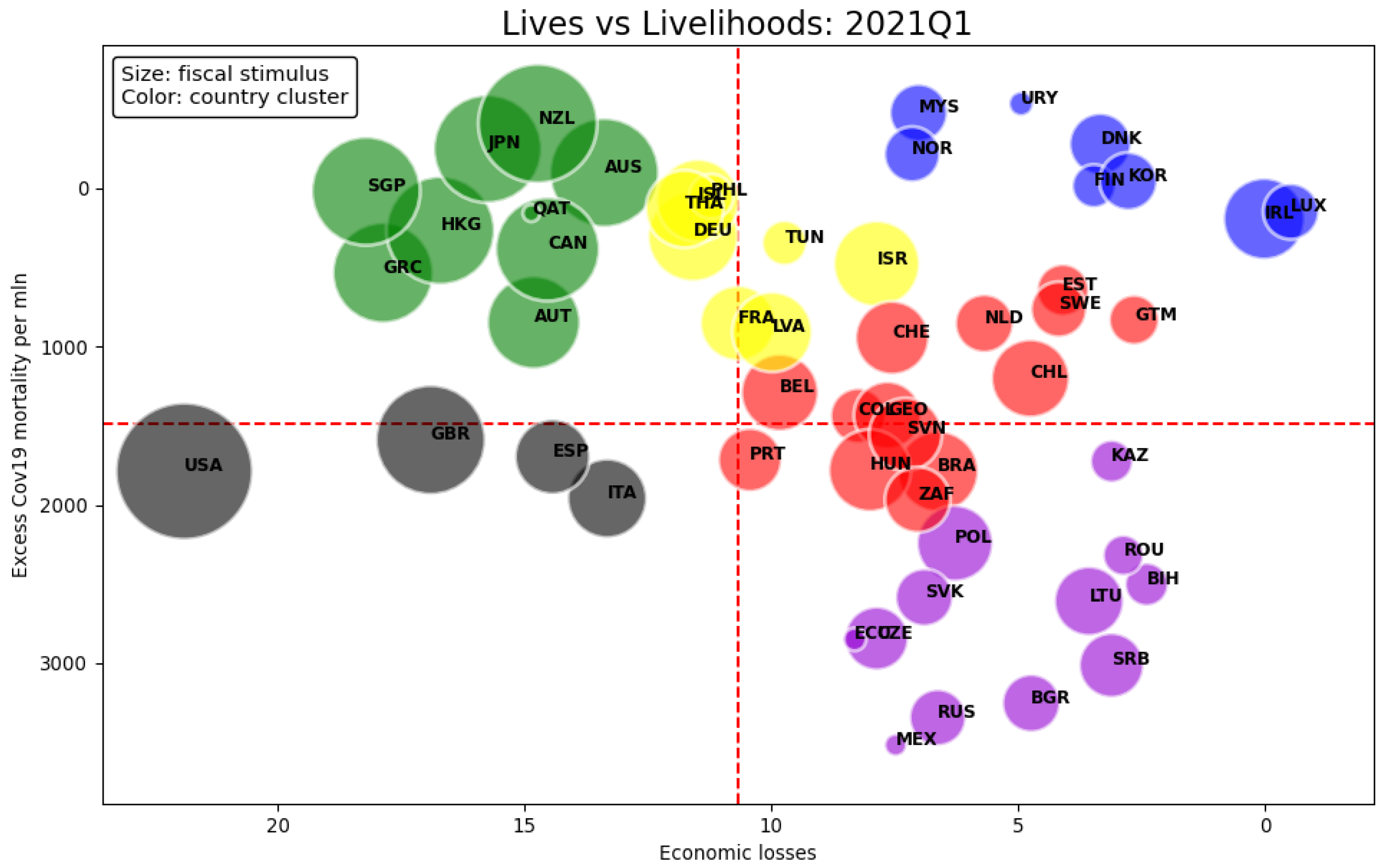
• Countries in the blue cluster display low economic losses and excess mortality at the same time. This group represents the most successful countries since they managed to reduce human and economic losses. Remarkably, a subgroup is made of Scandinavian countries (Denmark, Finland, and Norway) except Sweden, which places itself not too far from the blue one in the red cluster. This is a first indication that some structural characteristics common to the Scandinavian region helped to mitigate the impact of the outbreak, whereas divergences in mitigation policies resulted in a detachment of Sweden from the rest of Scandinavia.14
• The green cluster is characterized by mid to high economic losses but low excess mortality. Economic losses are determined foremost by additional fiscal spending as appears by the size of bubbles. Looking at the vertical axis, one can assert that mortality was mitigated by large fiscal expenditure which could be interpreted as evidence of governments’ effort to save lives as well as to provide economic relief (e.g., financing health policies such as testing and tracing, or compensating for lockdowns). It is worth noticing that most countries in the green cluster followed an elimination strategy. 15 For them, the trade-off between saving lives and the economy is clearly visible, although the same cannot be generalized to the rest of the countries. Furthermore, many Asian countries in our sample are included in the second quadrant, despite not all being in the green cluster. This may reflect cultural or other group-specific factors, such as preparedness or previous exposure to epidemics, supporting the argument that structural conditions matter.
• The gray group only includes Western countries with mid mortality and mid to high economic losses. These are especially driven by fiscal expenditure for the US and the UK. We interpret the cluster performance as the outcome of bad policies, even if Italy’s performance might have been worsened by being the first Western country to be impacted by COVID-19. The management of the pandemic by the US and UK governments was aimed to save the economy and partly neglected the severity and reach of COVID-19. As a consequence, the public expenditure by those countries was mostly addressed to support the economy, though a substantial regional heterogeneity cannot be ignored especially for the US. As such, the gray cluster shows economic losses fairly comparable with the green group, but worse mortality: policy interventions were not as effective.16
• The least successful cluster in mitigating mortality is the purple one.17 Countries belonging to Central and Eastern Europe, in particular to the former USSR and South America, are in the group or close to it. Excess mortality is the highest across all groups, but economic losses are low with limited fiscal expenditure. The measures adopted by the purple countries to contrast contagion appear insufficient or lacked the structural conditions to be put in place.18 This gives the idea that the spreading of the virus was out of control.
• The yellow and red clusters show a moderate variability in excess mortality and economic losses. The yellow group has on average lower mortality but greater economic losses than the red one. The two clusters do not display distinctive characteristics in the context of Figure 2 but take intermediate values. Thus, some countries display features similar to those of their neighboring clusters (DEU, PHL, ISL, THA, HUN, BRA, ZAF).

A couple of remarks from the observation of Figure 2: First, the fiscal stimulus provided by public expenditure in green and gray countries may lead, under unspecified conditions, to a faster recovery and higher economic growth in the aftermath, thus decreasing future economic losses. Second, even if the impact of spending on mortality is not precisely quantified, we observe that a large fiscal stimulus generally limited excess mortality compared to the worst group. Lastly, clustering analysis could be employed in a future extension of this study to group countries based on structural conditions or COVID-19 policies and to visualize if there are any clear patterns from these to clusters displayed in Figure 2.

4.2. LPM

The LPM is initially used to pinpoint significant structural conditions and policy measures in determining the probability of a country being assigned to the cluster of interest. Table 3 reports the LPM regression results. The discussion focuses on estimates which are significantly different from zero at the 5% significance level or below. Additionally, we restrict the analysis to the sign of correlation between different variables and outcomes. Results for each of the six regressions will be presented here.

In the blue group, the variable trade reliance on services is statistically correlated with the probability of being part of this cluster (low excess mortality and economic losses). Countries in the blue group have economies with a greater reliance on trade from services than others. This variable is a structural characteristic of an economy that facilitates a country’s ability to confront a pandemic, since trade from services can be safely carried out at home.19 We interpret this result as an incentive-compatible story. To the extent that governments want people to work from home, or people themselves want to minimize close contact with others, a larger country’s capacity for remote working reduces the cost of the governmental decision in terms of income and economic activity. Similarly, people are more likely to comply with any mandate to stay at home if they can easily transfer from an office to their house. With more people potentially working from home, the spread of the virus slows down, which translates into less excess mortality. As an example of why structural conditions matter, note that the group average of trade reliance on services is mostly driven by Ireland and Luxembourg. These two countries were not only able to implement stronger stay-at-home policies than others in the blue group, but also relative to other groups.20 In spite of this stringency, these two countries simultaneously registered the lowest economic losses of the whole sample and are part of the group with low excess mortality. Moreover, heavy trade reliance on services directly reduces economic losses, as the trade reliance on services is less disrupted during the pandemic compared to the trade of goods. Therefore, trade reliance on services is a desirable structural condition that saves lives and the economy.

Concerning policies, countries in the blue group spent little on non-health sectors compared to other countries and implemented limited stay-at-home orders. Since, in parallel, these countries registered low excess mortality as well as low economic losses, these results highlight that, in this exercise, correlation is not causation. With better performance in both excess mortality and economic losses, a government has lower incentives to spend excessively on non-health sectors to stimulate the economy, or to enforce strict lockdown rules. When a government continues to spend during the pandemic due to poor past health performance, we say a country has fallen into a “COVID trap.” Countries in the blue group successfully avoided the COVID trap due to early success and saved more fiscal space for other needs. Note that such policy decisions are consistent with the facilitating effect of addressing pandemics of an economic structure with heavy trade reliance on services.

For the yellow group, we did not find any significant variable determining the outcome. This indicates that the group does not have common structural conditions or policy measures associated with similar outcomes. Perhaps the countries in the yellow group reached their success with heterogeneous structural conditions and policy measures.

Countries in the green group have in common a greater past pandemic experience (SARS) than countries in other groups. Canada, Singapore, Australia, and New Zealand all suffered from the SARS pandemic to a great extent. Given that this group is characterized by low excess mortality, it is plausible that governments and individuals learned from the SARS pandemic, which helped the to be better prepared for COVID-19. Pandemic experience from SARS also helped countries in the green group to save more lives during the H1N1 pandemic. In terms of policy variables, countries in the green group spent heavily in non-health sectors compared to other countries. Greece, Singapore, Austria, Japan, and Canada suffered from relatively high GDP losses. Therefore, it is rational for their governments to spend heavily on non-health sectors to stimulate the economy. Unlike the blue group, the green group lacks a trade reliance on services, potentially resulting in heavy economic losses. Finally, non-health spending might have created incentives for firms to close down and for individuals to take on fewer risks by working less. This is a likely channel by which fiscal spending in non-health might have saved lives for countries in the green group.

The moderate outcomes of countries in the red group are associated with a mixed set of variables. Red countries show good structural conditions on average, such as low population density and cardiovascular death. However, a significant disadvantage is a heavy reliance on the trade of goods. Due to trade disruption, many countries in the red group directly suffered economically. In addition, a heavy reliance on the trade of goods might also increase transmission risk via transportation and logistics. This could lead to an increase in excess deaths. In terms of policies, countries in the red group did not implement enough internal movement restrictions. Belgium, Hungary, and Portugal either recommended not to travel internally or implemented no restrictions at all. Therefore, for the majority of the countries in the red group, more policies are needed to reduce the transmission risk through the trade of goods. Countries in the red group also spent heavily on health, further suggesting that their medical system was under severe pressure. Such an observation is consistent with the findings for countries in the gray group, which are explained below.

The UK, the US, Italy, and Spain form the gray group.21 The group has a good structural condition in terms of health and a low level of diabetes prevalence. The group average is mostly driven down by Italy and the UK. However, the US is ranked fourth in diabetes prevalence, thus making the estimate of the group coefficient less significant. The countries in the gray group have many poor structural conditions. First, they have a larger elderly population above the age of 70 and they do not have enough hospital beds. Italy and Spain have a large elderly population compared to others. Because the risk of death from COVID-19 might increase with age, elderly people might need more protection. The protection of elderly people variable measures elderly protection in care facilities. Italy implemented strict measures such as extensive restrictions relating to elderly isolation in care facilities. However, Spain did very little in terms of elderly protection. Policies implemented in Spain concerning the elderly were mostly recommendations rather than strict isolation or hygiene rules. This might have resulted in the failure of Spain to save elderly lives. The lack of hospital beds may also help to explain why the group suffered from high excess mortality. Lastly, the group has a high population density on average.22 High population density might increase transmission risks, leading to a higher number of COVID-19 deaths. This might be a potential factor that contributed to the moderate level of excess mortality for the UK and Italy. Surprisingly, the countries in the gray group implemented many policies in some of the policy criteria, but the results only hold at the 5% significance level. The group implemented many internal movement restrictions and spent heavily on health. Although people are banned from traveling between cites or states, there are several reasons for the policy to fail. First, people might move intensively before or after new restrictions begin. Second, law enforcement might fail to enforce restrictions. People have less incentive to travel if they stay in their preferred locations during the restriction period. Perhaps policies are needed to help people move slowly and safely, both before and after the restriction period. Such incentive-compatible policy design should also reduce law enforcement costs and relieve law enforcement pressure. Finally, the UK, the US, and Spain spent heavily on health compared to other countries.23 There is no denying that more spending on health should help reduce excess deaths. However, there might be diminishing returns. Labor and capital supply in health are difficult to match to a sudden rise in demand in the short term, despite heavy spending in health.24 A lack of hospital beds for all countries in the gray group further supports this point. Most importantly, lengthy and frequent health spending indicates that the medical system was under severe pressure due to poor health outcomes in the past. Countries should avoid falling into such a “COVID trap” by using policy tools other than excessive additional fiscal stimulus in health.

Finally, we did not find significant structural conditions or policy measures associated with the outcomes of countries in the purple group. This might be because we excluded the most relevant structural condition for the purple group, which is corruption, a variable dropped for reducing multicollinearity.

4.3. LASSO and Logit Regression

This section presents the results of logistic LASSO and logit regression. To recall our strategy, we first use LASSO to select variables for reducing dimensionality and preparing for the logistic regression. As a second step, LASSO-selected variables are included as regressors in the logistic regression to determine the statistically significant variables affecting the outcomes. The logistic LASSO results are reported in Table 4.

For the blue group, seven variables are selected. In this group, countries have fewer smokers, rely more on the trade of services, and are less corrupted on average. In terms of policies, countries in the blue group implemented more testing policies. Additionally, they did not apply a strong facial covering policy and spent very little in the health and non-health sectors.

The results on trade reliance and fiscal spending are consistent with the LPM findings. Here, we focus on interpreting the new results. A smaller smoking population could be a desirable structural condition for the blue group. Other studies have also found that smoking could increase the risk of experiencing severe COVID-19 related infection, hospitalization, and death (Clift et al. 2022; Sanchez-Ramirez and Mackey 2020). Moreover, having a less corrupted government might lead to policies being implemented more efficiently and effectively. Since policy variables reflect policy announcements, the less corrupted governments are more likely to comply with the announced policies, thus saving more lives. Additionally, fiscal spending is more likely to be effectively allocated, with a lower chances of being embezzled. Beyond less corruption, many countries in the blue group, such as South Korea, Malaysia, Denmark, and Luxembourg, have all implemented many testing policies. They have introduced open public testing, such as drive-through testing, which is available to people with COVID-19 symptoms. People who test positive self-isolate, thus stopping the virus from spreading. Additionally, testing provides COVID-19 information to the government and individuals, informing their decisions on policies and individual behaviors. Therefore, a reliable and efficient testing system is crucial for laying down the foundation for success. Finally, countries in the blue group did not strongly implement facial covering policies. The success of such policies largely depends on how individuals respond to them. If people wear masks and follow social distancing rules themselves, there is less need for the government to tighten rules and enforce them. Additionally, favorable results from past experiences might lead to weaker facial covering rules. It would be interesting to investigate how individuals living in countries in the blue group protected themselves during the pandemic. Nevertheless, it would be misleading to conclude that looser facial covering policies lead to success in saving lives.

The robustness of the LPM results is proven by the variables selected for the green cluster, namely SARS experience and fiscal stimulus in non-health. No variables are chosen for the yellow group. Again, this suggests that the heterogeneity in the yellow group prevents regression analysis from recognizing any common conditions or behavior in the group. The success model for the yellow group is not as clear as for the green or blue groups: being characterized by diverse structural conditions and having applied various policies portfolios, the yellow group achieved moderate success via different paths. Countries in the red group have a less educated population on average, and implemented more stay-at-home orders. For some countries, such as Portugal and Belgium, a large share of the population older than 70 displays a low level of education. As mean years of schooling can be used to track the average level of education for those aged 25 and above, age might be the underlying factor causing higher excess deaths in these countries. However, countries such as Brazil and Colombia tend to have a lower level of education for all age groups. It is not straightforward to see the relationship between education, excess mortality, and GDP loss, as income could be a confounding variable. Brazil and Colombia have a relatively high Gini coefficient, further proving this point. All in all, the cause of failure in the red group could be summarized by a larger vulnerable population, characterized by elderly or low-income people. Did countries in the red group design policies to best protect their vulnerable population? Portugal and Belgium only implemented moderate to low levels of elderly-protection policies. Brazil and Colombia did announce a moderate to a high level of fiscal spending on non-health sectors. However, they are also the most corrupted countries in the sample, meaning that the low-income population might not have received all of the promised financial support. Poor health outcomes in the past led to many stay-at-home orders being implemented for countries in the red group. Bad outcomes thus repeatedly appear as soon as restrictions are lifted. Countries in the red group therefore entered into the “COVID trap”. More lives could have been saved if policies were designed to best protect their unusually large vulnerable population. Even though short-term COVID-19 policies such as lockdowns might work to reduce new cases and deaths, for economic reasons, countries will inevitably lift restrictions. As a result, the issues connected to structural conditions and a lack of proper policies such as testing will return, potentially increasing excess mortality again.

The most relevant factors among the gray group are past H1N1 experience and fiscal stimulus in health. The US, UK, Spain, and Italy all suffered from H1N1. However, judging by their COVID-19 outcomes, their governments and the individuals did not learn much from the H1N1 pandemic experience. These countries spent heavily on health, consistent with the findings from the LPM results.

Finally, countries in the purple group have a higher cardiovascular death rate and are more corrupted on average. People with cardiovascular diseases might find it difficult to access emergency services during the pandemic. This increases the number of indirect deaths caused by COVID-19 due to the collapse of the medical system. Secondly, people with cardiovascular diseases might be less likely to survive severe COVID-19 symptoms. The two reasons combined make the cardiovascular death rate a potential causal structural condition in determining failure. In contrast to the blue group, countries in the purple group are deeply corrupted. Corruption may signal that policy announcements do not truly reflect the actual policies being announced. Additionally, the effective fiscal spending received by households, firms, and health institutions might be much lower than reported. These could be the potential reasons for the lack of any significant policy factor in the purple group.

Table 5 reports the logistic regression results using variables selected by LASSO. For the blue group, the facial coverings coefficient is significant at 5%. Testing and trade reliance on services are significant at 10%.25 Therefore, the most consistent group behavior for the blue group is the implementation of fewer facial covering policies than others. For the green group, fiscal stimulus in non-health is significant at the 1% level. For the red group, the stay-at-home order variable is significant at a 5% significance level. Due to poor outcomes in the past, countries in the red group repeatedly introduce strict stay-at-home orders. There are no significant coefficient estimates for the gray group. Finally, cardiovascular death rate and corruption both show significance at the 10% level for the purple group. When analyzing the results across all groups, we found that consistent policy decisions are mostly the rational consequences of past outcomes. This cannot directly explain how each group succeeded or failed in the long run. Testing and fiscal stimulus in non-health sectors are exceptions. A robust testing system is a foundation for long-term success, as testing provides crucial information which might influence behaviors. Continuous non-health spending gives individuals and firms an incentive to take on fewer risks during the pandemic. Both policies come with an immediate economic cost when implemented. However, they also help save lives and reduce economic costs in the long term. Structural conditions also have a long-term impact on outcomes. The most successful countries rely more on the trade of services. The least successful countries suffer from corruption and a high cardiovascular death rate. Countries should utilize their good structural conditions by designing policies around them. Policies are also needed for tackling poor structural conditions to avoid the long-term failure to save lives and the economy. Corruption is perhaps the most difficult structural condition to be dealt with as it reduces the incentive for the government to save lives or reduce economic losses.

5. Discussion

The first result discussed here connects to the research question asking how countries performed during the pandemic, judged by their health and economic outcomes. Our findings show that overall there is no negative correlation between health and economic outcomes. In other words, looking at all countries in our sample, there is no trade-off between saving lives and the economy. If there were a trade-off, we would see countries spread along the diagonal that crosses Figure 2 from North-West to South-East. The heterogeneity in performances we observe might be generated by the interaction of governments’ policies with countries’ characteristics. Such an interaction could also explain the deviation of actual outcomes from intended policy objectives. However, some countries performed better than others, as they emerged from the cluster analysis. In particular, the blue group showed low human and economic losses. This result is surprising, as all countries except South Korea followed mitigation strategies, namely they did not deliberately decide to suppress the virus. These countries may have reacted swiftly (especially Norway, Denmark, and Finland) adopting non-pharmaceutical policies that prevented contagion soaring uncontrolled. Nevertheless, our findings do not support the thesis that mitigation is dominated by elimination strategies (Oliu-Barton et al. 2021). Rather, we notice a broad spectrum in the implementation of mitigation strategies ranging from countries that reacted soon and vehemently to those that preferred to invest in economic stimulus rather than stopping the contagion. Combined with structural characteristics, it produces diverse performances on the XY plane. Concerning elimination strategies, we observed that countries tend to cluster together into the green group. These countries managed to limit excess mortality but at the price of higher economic costs. As we include fiscal stimulus to GDP growth to account for losses, our results suggest that elimination strategies are effective in saving lives but entail high economic costs, especially in terms of future repayments. Thus, contrary to (Baker et al. 2020; Oliu-Barton et al. 2021), we do not find evidence that elimination is the optimal response strategy to COVID-19. Finally, the performances of the US and the UK can be interpreted in agreement with Alvelda et al. (2020). The US and UK moved from North-East to South-West on the diagonal in a negative feedback loop where the size of the fiscal stimulus needed to support economic activity increased in step with contagion. The accumulation of economic and human losses continued until lockdowns were unavoidable to abate contagion, moving those countries to the left of the diagonal.

The second research question seeks to find the drivers behind the success and failures. Based on the attributes found in the econometric analysis, we can give the following policy recommendations for future pandemic preparations. First, governments should design health and economic policies based on structural conditions. A sizable vulnerable population deserves special attention. The governments should incentivize the low-income population to take fewer risks during the pandemic. They should be working less in environments with high transmission risks. Such a conclusion was also reached in Wildman (2021). Moreover, the elderly population should be best protected, especially if they live in care facilities with others. Bourdin et al. (2022) found European governments might have noticed the death increase in care homes and responded by increasing restrictions. Additionally, people with vulnerable health conditions such as cardiovascular disease or smoking habits should be protected and given extra warnings (Clift et al. 2022; Sanchez-Ramirez and Mackey 2020). Second, governments should consider providing open public testing nationally to those who show symptoms. Additional fiscal stimulus in non-health could incentivize individuals and businesses to comply with strict pandemic rules, which might save lives and reduce excessive economic losses.26 Finally, corruption might reduce effective policy implementations. In Islam et al. (2020), the case study of South Africa confirms such finding to an extent. Countries suffering from corruption, such as those in the purple group, should fight corruption and improve government transparency.

It should be noted that the scope of our analysis should not be interpreted as aiming to provide a normative valuation of the responses undertaken by governments. Rather, we show that a one-size-fits-all solution does not exist (Bourdin et al. 2022), and countries’ performances result from the interaction of policies and structural conditions. Our analysis tried to capture some common factors by country group, which matter ex-post. While these can certainly be accounted for in the formulation of policy responses, there is still considerable heterogeneity within each cluster. Therefore, at the high level, we recommend that short-term policies should take into account the country’s characteristics, but above all, on a longer horizon, governments should work on resilience and robustness by enhancing country-specific structural conditions.

There are some limitations of the analysis, which could inspire future research. First, vaccination is not included as a policy instrument. Because the sample was taken from January 2020 to March 2021, the majority of the population was not vaccinated in all countries. Future research studying samples beyond March 2021 should consider the effectiveness of vaccination in saving lives and the economy. Second, regional effects within countries are not investigated in this study. For many countries, such as the US, policies were implemented differently at a regional level. Each region might have different structural conditions in determining its health and economic performance. The analysis of a specific country at the regional level might bring new insights. Third, the results found that additional fiscal stimulus in non-health sectors might have saved lives and the economy. However, we know little about which part of the spending effectively contributed to desirable health and economic outcomes. Future research should help to identify effective spending and to distinguish it from ineffective spending, suffering from diminishing returns in reaching desirable outcomes. Furthermore, although the study used a variety of factors that might potentially determine the outcomes, more attributes could still be found. For example, countries tend to cluster based on the nature of their healthcare systems. Therefore, countries with a similar design in terms of their healthcare systems could theoretically generate a similar performance during the pandemic, if controlled for other factors.

6. Conclusions

This paper investigates the structural conditions and policy decisions affecting the lives and livelihood outcomes in selected countries during the COVID-19 pandemic. In order to do so, we have proceeded in two steps. First, we presented a hierarchical clustering analysis, grouping countries with similar health and economic performances without the need of having a normative statement on the value of lives versus economic activity. In this way, we could smooth the process of drawing insights into the relationship between outcomes, structural features, and policies, which was the primary goal of this investigation. Second, following the clustering analysis, we proceeded with a regression analysis, the main objective of which was to identify significant attributes in increasing the probability of a country being assigned to each group with different health and economic outcomes. Accordingly, some conclusions could be drawn:

First, we found no evidence supporting the existence of a trade-off between lives and livelihoods across our sample. Indeed, the best-performing group had relatively low excess mortality and GDP losses when additional fiscal stimulus was adjusted for. Above all, the position of countries in the bi-dimensional plane does not always reflect their initial strategies. Second, the results suggest that three structural conditions are of most importance: trade reliance on services, corruption, and the size of the vulnerable population. Countries heavily relying on the trade of services are most likely to survive strict COVID-19 restrictions and bear a lower economic cost in the long run. Corrupted countries might suffer from insufficient and ineffective policy implementations, costing lives and living standards. The elderly, low-income, and cardiovascular-failing population should be the most protected, as they are too vulnerable to survive the pandemic. Finally, policies such as implementing large-scale open public testing and additional fiscal spending on non-health sectors could help reduce excess mortality, preventing unnecessary economic losses.

References

1. Acemoglu, Daron, Victor Chernozhukov, Iván Werning, and Michael D. Whinston. 2021. Optimal targeted lockdowns in a multigroup sir model. American Economic Review: Insights 3: 487–502. [Google Scholar] [CrossRef]
2. Alvarez, Fernando, David Argente, and Francesco Lippi. 2021. A simple planning problem for COVID-19 lock-down, testing, and tracing. American Economic Review: Insights 3: 367–82. [Google Scholar] [CrossRef]
3. Alvelda, Phillip, Thomas Ferguson, and John C. Mallery. 2020. To save the economy, save people first. INET Blog, November 18. [Google Scholar]
4. Arias, Jonas E., Jesús Fernández-Villaverde, Juan Rubio Ramírez, and Minchul Shin. 2021. The Causal EffEcts of Lockdown Policies on Health and Macroeconomic Outcomes; Working Paper 28617; Cambridge: National Bureau of Economic Research. [CrossRef]
5. Baker, Michael G., Nick Wilson, and Tony Blakely. 2020. Elimination could be the optimal response strategy for COVID-19 and other emerging pandemic diseases. BMJ 371: m4907. [Google Scholar] [CrossRef] [PubMed]
6. Barbieri Góes, Maria Cristina, and Ettore Gallo. 2021. Infection Is the Cycle: Unemployment, Output and Economic Policies in the COVID-19 Pandemic. Review of Political Economy 33: 377–93. [Google Scholar] [CrossRef]
7. Basher, Syed Abul, and A. K. Enamul Haque. 2021. Public policy lessons from the COVID-19 outbreak: How to deal with it in the postpandemic world? Journal of Social and Economic Development 23: 234–47. [Google Scholar] [CrossRef]
8. Blair, Alicia, Mattia de Pasquale, Valentin Gabeff, Mélanie Rufi, and Antoine Flahault. 2022. The end of the elimination strategy: Decisive factors towards sustainable management of COVID-19 in New Zealand. Epidemiologia 3: 135–47. [Google Scholar] [CrossRef]
9. Boitan, Iustina A., Emilia M. Câmpeanu, and Sanja S. Mališ. 2021. Economic sentiment perceptions during COVID-19 pandemic—A european cross-country impact assessment. Amfiteatru Economic 23: 982–1002. [Google Scholar]
10. Bourdin, Sébastien, John Moodie, András Igar, and Mounir Amdaoud. 2022. Territorial Impacts of COVID-19 and Policy Answers in European Regions and Cities. Report. Luxembourg: European Observation Network for Territorial Development and Cohesion. [Google Scholar]
11. Bourdin, Sebastien, Slimane Ben Miled, and Jamil Salhi. 2022. The drivers of policies to limit the spread of COVID-19 in europe. Journal of Risk and Financial Management 15: 67. [Google Scholar] [CrossRef]
12. Brodeur, Abel, David Gray, Anik Islam, and Suraiya Bhuiyan. 2021. A literature review of the economics of COVID-19. Journal of Economic Surveys 35: 1007–44. [Google Scholar] [CrossRef]
13. Chetverikov, Denis, Zhipeng Liao, and Victor Chernozhukov. 2021. On cross-validated lasso in high dimensions. The Annals of Statistics 49: 1300–17. [Google Scholar] [CrossRef]
14. Clift, Ashley K., Adam Von Ende, Pui San Tan, Hannah M. Sallis, Nicola Lindson, Carol A. C. Coupland, Marcus R. Munafò, Paul Aveyard, Julia Hippisley-Cox, and Jemma C. Hopewell. 2022. Smoking and COVID-19 outcomes: An observational and mendelian randomisation study using the uk biobank cohort. Thorax 77: 65–73. [Google Scholar] [CrossRef]
15. Daumann, Frank, Florian Follert, Werner Gleißner, Endre Kamarás, and Chantal Naumann. 2021. Political decision-making in the COVID-19 pandemic: The case of germany from the perspective of risk management. International Journal of Environmental Research and Public Health 19: 397. [Google Scholar] [CrossRef] [PubMed]
16. Delli Gatti, Domenico, and Severin Reissl. 2022. Agent-based covid economics (abc): Assessing non-pharmaceutical interventions and macro-stabilization policies. Industrial and Corporate Change 31: 410–47. [Google Scholar] [CrossRef]
17. Dingel, Jonathan I., and Brent Neiman. 2020. How many jobs can be done at home? Journal of Public Economics 189: 104235. [Google Scholar] [CrossRef] [PubMed]
18. ECDC. 2010. The 2009 a(h1n1) Pandemic in Europe. Report. Stockholm: European Centre for Disease Prevention and Control. [Google Scholar]
19. Fang, Hanming, Long Wang, and Yang Yang. 2020. Human mobility restrictions and the spread of the novel coronavirus (2019-ncov) in china. Journal of Public Economics 191: 104272. [Google Scholar] [CrossRef]
20. Freijeiro-González, Laura, Manuel Febrero-Bande, and Wenceslao González-Manteiga. 2022. A critical review of lasso and its derivatives for variable selection under dependence among covariates. International Statistical Review 90: 118–45. [Google Scholar] [CrossRef]
21. Friedson, Andrew I., Drew McNichols, Joseph J. Sabia, and Dhaval Dave. 2020. Did California’s Shelter-in-Place Order Work? Early Coronavirus-Related Public Health Effects. Working Paper 26992. Cambridge: National Bureau of Economic Research, April. [Google Scholar] [CrossRef]
22. Gan, Guojun, Chaoqun Ma, and Jianhong Wu. 2020. Data Clustering: Theory, Algorithms, and Applications. Philadelphia: Society for Industrial and Applied Mathematics. [Google Scholar]
23. Geodatasource. 2022. Country Borders. Available online: https://www.geodatasource.com/addon/country-borders (accessed on 1 August 2022).
24. Ghosh, Jayanta K. 2012. Statistics for high-dimensional data: Methods, theory and applications by peter bühlmann, sara van de geer. International Statistical Review 80: 486–7. [Google Scholar] [CrossRef]
25. Hale, Thomas, Noam Angrist, Rafael Goldszmidt, Beatriz Kira, Anna Petherick, Toby Phillips, Samuel Webster, Emily Cameron-Blake, Laura Hallas, Saptarshi Majumdar, and et al. 2021. A global panel database of pandemic policies (oxford COVID-19 government response tracker). Nature Human Behaviour 5: 529–38. [Google Scholar] [CrossRef]
26. Haug, Nils, Lukas Geyrhofer, Alessandro Londei, Elma Dervic, Amélie Desvars-Larrive, Vittorio Loreto, Beate Pinior, Stefan Thurner, and Peter Klimek. 2020. Ranking the effectiveness of worldwide COVID-19 government interventions. Nature Human Behaviour 4: 1303–12. [Google Scholar] [CrossRef]
27. IMF. 2021. Fiscal Monitor Database of Country Fiscal Measures in Response to the COVID-19 Pandemic. Available online: https://www.imf.org/en/Topics/imf-and-covid19/Fiscal-Policies-Database-in-Response-to-COVID-19 (accessed on 1 August 2022).
28. Islam, S. Nazrul, Hoi Wai Jackie Cheng, Kristinn Sv. Helgason, Nicole Hunt, Hiroshi Kawamura, and Marcelo LaFleur. 2020. Variations in COVID Strategies: Determinants and Lessons. Working Paper 172. New York: United Nations, Department of Economic and Social Affairs. [Google Scholar]
29. Karlinsky, Ariel, and Dmitry Kobak. 2021. Tracking excess mortality across countries during the COVID-19 pandemic with the world mortality dataset. eLife 10: e69336. [Google Scholar] [CrossRef]
30. Kochańczyk, Marek, and Tomasz Lipniacki. 2021. Pareto-based evaluation of national responses to COVID-19 pandemic shows that saving lives and protecting economy are non-trade-off objectives. Scientific Reports 11: 2425. [Google Scholar] [CrossRef]
31. König, Michael, and Adalbert Winkler. 2021. The impact of government responses to the COVID-19 pandemic on gdp growth: Does strategy matter? PLoS ONE 16: e0259362. [Google Scholar] [CrossRef]
32. Le Cessie, Saskia, and Johannes C. Van Houwelingen. 1992. Ridge estimators in logistic regression. Journal of the Royal Statistical Society: Series C (Applied Statistics) 41: 191–201. [Google Scholar] [CrossRef]
33. Long, Han, Chun-Ping Chang, Sujeetha Jegajeevan, and Kai Tang. 2022. Can central bank mitigate the effects of the COVID-19 pandemic on the macroeconomy? Emerging Markets Finance and Trade 58: 2652–69. [Google Scholar] [CrossRef]
34. Ludvigson, Sydney C., Sai Ma, and Serena Ng. 2020. COVID-19 and the Macroeconomic Effects of Costly Disasters. Working Paper 26987. Cambridge: National Bureau of Economic Research. [Google Scholar] [CrossRef]
35. Maloney, William F., and Temel Taskin. 2020. Determinants of Social Distancing and Economic Activity during COVID-19: A Global View. Working Paper 9242. Washington: The World Bank. [Google Scholar]
36. Miguel, Edward, and Ahmed Mushfiq Mobarak. 2021. The Economics of the COVID-19 Pandemic in Poor Countries. Working Paper 29339. Cambridg: National Bureau of Economic Research. [Google Scholar] [CrossRef]
37. Murtagh, Fionn, and Pedro Contreras. 2017. Algorithms for hierarchical clustering: An overview, II. Wiley Interdisciplinary Reviews: Data Mining and Knowledge Discovery 7: e1219. [Google Scholar] [CrossRef] [Green Version]
38. OECD. 2022. Income Inequality. Available online: https://data.oecd.org/inequality/income-inequality.htm (accessed on 1 August 2022).
39. Oliu-Barton, Miquel, Bary S. R. Pradelski, Philippe Aghion, Patrick Artus, Ilona Kickbusch, Jeffrey V. Lazarus, Devi Sridhar, and Samantha Vanderslott. 2021. Sars-cov-2 elimination, not mitigation, creates best outcomes for health, the economy, and civil liberties. The Lancet 397: 2234–6. [Google Scholar] [CrossRef]
40. Our World in Data. 2022a. Death Rate from Cardiovascular Disease. 2017. Available online: https://ourworldindata.org/grapher/cardiovascular-disease-death-rates?time=2017 (accessed on 1 August 2022).
41. Our World in Data. 2022b. Diabetes Prevalence, 2017. Available online: https://ourworldindata.org/grapher/diabetes-prevalence?time=2017 (accessed on 1 August 2022).
42. Our World in Data. 2022c. Share of the Population that is 70 Years and Older. Available online: https://ourworldindata.org/grapher/share-of-the-population-that-is-70-years-and-older (accessed on 1 August 2022).
43. Phillips, Nicky. 2021. The coronavirus is here to stay-here’s what that means. Nature 590: 382–4. [Google Scholar] [CrossRef]
44. Rampini, Adriano A. 2020. Sequential Lifting of COVID-19 Interventions with Population Heterogeneity. Working Paper 27063. Cambridge: National Bureau of Economic Research. [Google Scholar] [CrossRef]
45. Sanchez-Ramirez, Diana C., and Denise Mackey. 2020. Underlying respiratory diseases, specifically copd, and smoking are associated with severe COVID-19 outcomes: A systematic review and meta-analysis. Respiratory Medicine 171: 106096. [Google Scholar] [CrossRef]
46. Sheridan, Adam, Asger Lau Andersen, Emil Toft Hansen, and Niels Johannesen. 2020. Social distancing laws cause only small losses of economic activity during the COVID-19 pandemic in scandinavia. Proceedings of the National Academy of Sciences 117: 20468–73. [Google Scholar] [CrossRef]
47. The World Bank. 2022a. Hospital Beds (per 1000 People). Available online: https://data.worldbank.org/indicator/SH.MED.BEDS.ZS (accessed on 1 August 2022).
48. The World Bank. 2022b. Physicians (per 1000 People). Available online: https://data.worldbank.org/indicator/SH.MED.PHYS.ZS (accessed on 1 August 2022).
49. The World Bank. 2022c. Population Density (People per sq. km of Land Area). Available online: https://data.worldbank.org/indicator/EN.POP.DNST (accessed on 1 August 2022).
50. The World Bank. 2022d. Prevalence of Current Tobacco use (Percent of Adults). Available online: https://data.worldbank.org/indicator/SH.PRV.SMOK (accessed on 1 August 2022).
51. The World Bank. 2022e. Trade in Services (Percent of GDP). Available online: https://data.worldbank.org/indicator/BG.GSR.NFSV.GD.ZS (accessed on 1 August 2022).
52. The World Bank. 2022f. Trade (Percent of GDP). Available online: https://data.worldbank.org/indicator/NE.TRD.GNFS.ZS (accessed on 1 August 2022).
53. Tibshirani, Robert. 1996. Regression shrinkage and selection via the lasso. Journal of the Royal Statistical Society: Series B (Methodological) 58: 267–88. [Google Scholar] [CrossRef]
54. Transparency International. 2022. Corruption Perception Index 2019. Available online: https://www.transparency.org/en/cpi/2019 (accessed on 1 August 2022).
55. WHO. 2015. Summary of Probable Sars Cases with Onset of Illness from 1 November 2002 to 31 July 2003. Available online: https://www.who.int/publications/m/item/summary-of-probable-sars-cases-with-onset-of-illness-from-1-november-2002-to-31-july-2003 (accessed on 1 August 2022).
56. Wildman, John. 2021. COVID-19 and income inequality in oecd countries. The European Journal of Health Economics 22: 455–62. [Google Scholar] [CrossRef]
57. Zhao, Peng, and Bin Yu. 2006. On model selection consistency of lasso. The Journal of Machine Learning Research 7: 2541–63. [Google Scholar]
58. Zhao, Sen, Daniela Witten, and Ali Shojaie. 2021. In Defense of the Indefensible: A Very Naïve Approach to High-Dimensional Inference. Statistical Science 36: 562–77. [Google Scholar] [CrossRef]
59. Zou, Hui, and Trevor Hastie. 2005. Regularization and variable selection via the elastic net. Journal of the Royal Statistical Society: Series B (Statistical Methodology) 67: 301–20. [Google Scholar] [CrossRef] [Green Version]
Figure 1. Scree plot for HAC.
Jrfm 15 00354 g001
Figure 2. Economic losses (x-axis) and excess COVID-19 mortality per million people (y-axis) at 2021Q1. Note: Bubble size reflects countries’ additional fiscal spending compared to before the outbreak. Color groups are based on hierarchical clustering analysis. The red dashed lines are traced at mid points.
Jrfm 15 00354 g002