R&D, Industrial Policy and Growth

Abstract

An issue with estimating the impact of industrial support is that the firms that receive support may be politically connected, introducing omitted variable bias. Applying fixed-effects regressions on Vietnamese panel data containing several proxies for political connectedness to correct this bias, we find that firms that receive industrial support in the form of tax holidays experience more rapid productivity growth, particularly in R&D-intensive industries, and less so among politically connected firms. These findings do not appear to be due to the presence of financing constraints. We then develop a second-generation Schumpeterian growth model with many industries, and show that tax holidays disproportionately raise productivity growth in R&D-intensive industries. These results are significant and important for governments, especially those in transition and developing countries, in better targeting their industrial policy to facilitate higher productivity growth.

1. Introduction

Industrial policy is common around the world, yet the mechanisms through which industrial support might affect firms are not fully understood. In developing economies, industrial support has recently been found to improve industry performance (Aghion et al. 2015; Lin 2003). Questions remain, for example, as to whether industrial support encourages growth by stimulating innovation, or whether industrial support enables firms to overcome financing constraints. A confounding factor is that industrial support may not be exogenous: politically connected firms may be more likely to receive support, leading to omitted variable bias—particularly in a developing country context (Khwaja and Mian 2005; Li et al. 2008).

We identify the channels through which industrial support affects economic outcomes by focusing on industry variation. It is known since at least Cobb and Douglas (1928) that industries vary in the technology of production: for example, the production of Machinery is more capital-intensive and more R&D-intensive than the production of Textiles. By examining which technological characteristics interact with industrial support, we narrow down the key channels whereby industrial support affects firm performance.

We address the problem of omitted variable bias by using a firm-level panel database from Vietnam. Vietnamese data are particularly useful because they contain multiple proxies we can use to measure the political connectedness of firms. In addition, the use of panel data allows us to condition on firm-level fixed effects, which powerfully conditions on any idiosyncratic firm-level characteristics that might affect productivity, observed or otherwise.

We find that industrial support, measured using tax holidays as in Aghion et al. (2015), raises firm productivity growth.1 Tellingly, we find that it particularly raises productivity growth for firms in R&D-intensive industries. This suggests that the appropriate class of models for understanding the impact of industrial support on economic growth is the class of R&D-based growth models. Our finding is consistent with Ang and Madsen (2011), who find that R&D-based growth models are the class of models most consistent with the growth experience of the East Asian “miracle” economies. Interestingly, we do not find that industrial support particularly raises the productivity of firms in industries that might be expected to suffer from financing constraints. This indicates that our results concerning R&D are likely due to channels that do not involve financing constraints.2 We also find that industrial support is less beneficial to politically connected firms, underlining the importance of conditioning on connections.

Finally, we develop a general equilibrium R&D-driven growth model with many industries, extending the one-sector framework of Howitt (1999), in order to show that R&D-based growth models can broadly account for our empirical findings. In the model, we show that industrial support encourages productivity growth particularly among firms that are in R&D-intensive industries, as in the data. This is so even though there are no financing constraints in the model. Instead, it occurs simply because lower taxes increase the returns to successful R&D. This is so even though the model does not display scale effects. We conclude that industrial support mainly encourages growth by increasing the return to R&D, rather than by alleviating financing constraints that might hinder R&D, and that politically connected firms are less likely to benefit from this support.

Our paper relates to several bodies of literature as detailed in Section 1.1 below, including those on industrial policy and political connections. Aghion et al. (2015) explore industrial policy in China, and Acemoglu et al. (2018) develop and calibrate a model in which operational subsidies that target innovation by highly productive firms may improve welfare. Harrison et al. (2019) find that both state owned enterprises (SOEs) and former SOEs in China, while still having access to government assistance, fall behind private firms in terms of productivity. Fang et al. (2018) find that removing opportunities for corruption makes subsidies more effective at stimulating innovation.

Section 2 describes the sources of data, and provides details on our empirical strategy. Section 3 reports empirical results and the main robustness checks. Section 4 describes the model economy and its equilibrium. Section 5 concludes.

1.1. Related Literature

1.1.1. Literature on Industrial Policy

In the extensive literature on industrial policy, most studies pursue one of two approaches.

A first approach is qualitative, offering a historical perspective into the stages of development of different economies to generate policy frameworks that might explain their growth experiences (Amsden 1992; Chang 2002; Lin 2003; Wade 1990).

More recent work on industrial policy examines links between industrial policy and economic development using quantitative tools. For example, Aghion et al. (2015) explore industrial policy in the context of the Chinese economy among large and medium enterprises between 1998 and 2007. They show that industrial policies targeted at competitive sectors or aimed at promoting competition improve productivity growth.3 They argue that such industries benefit from support because competitive pressure motivates firms to innovate in order to differentiate horizontally, which in turn fosters productivity growth. This contrasts with the consensus regarding industrial policy in more developed economies, which is generally viewed as having reduced productivity by propping up failing firms—see Leonard and Van Audenrode (1993), Samaniego (2006) and Ranasinghe (2014).

Meanwhile, Acemoglu et al. (2018) use U.S. Census micro data to estimate the parameters of a model of firm-level innovation, productivity growth and reallocation with endogenous entry and exit. They show that industrial policy subsidizing the operations of existing firms that are of “low type” in terms of innovative capacity would negatively affect growth and aggregate welfare. Their policy experiment of a subsidy of 5 percent of GDP for incumbent firms’ operations leads to a reduction in welfare of about $1.5$ percent because it deters entry by new “high-type” firms. Meanwhile, a reduction of subsidies to low-type firms coupled with an increase in financial support to R&D activities of high-type firms encourages the entry of more productive firms and the exit of low-type firms. Their paper places a strong emphasis on innovation, and recommends the type of industrial policy that focuses on subsidizing R&D by highly productive firms. This argument is echoed by Boeing et al. (2016) who find that R&D spending had a positive effect on the productivity of publicly listed Chinese firms in the 2001–2011 period.

1.1.2. Literature on Political Connections

Also using Chinese data, Harrison et al. (2019) find that, while private firms that used to be state owned enterprises (SOEs) still have better access to government assistance compared to private firms, both privatized SOEs and SOEs fall behind private firms in their profitability. These results suggest that industrial support may be endogenous: firms that have ties with the government tend to get more state support, yet these firms may be less productive or have other characteristics related to outcome variables. This indicates the importance of conditioning on political connectedness when estimating the impact of industrial support.

Akcigit et al. (2018) present further evidence that businesses with political connections tend to perform worse than average. They develop a model of firm dynamics in which firms face a tradeoff between investing in innovation and strengthening their political connections. Using Italian data from 1993 to 2014, they find that firm-level political connections are ubiquitous, especially among large enterprises. However, industries with more politically connected firms are found to have weaker productivity growth. They also find that the firms that lead the market are much more likely to invest in political connections and less likely to innovate. Together, these findings suggest that the productivity impact of industrial support depends on the stage of development, and on the presence of political connections.

Additionally, some studies have uncovered evidence that firms with political connections enjoy better access to financing. For example, Rand (2017) find in Vietnamese small and medium enterprise data that political connectedness, proxied by Communist party membership of the owner or manager of each firm, decreases the likelihood of firms being credit-constrained. Li et al. (2008) find that political connections improve Chinese firms’ access to loans from banks and other state institutions, and that private firms with political connections perform better after controlling for human capital and other variables. Their paper concludes that political connections have a positive impact on firm performance in countries with weaker market institutions and legal frameworks. Meanwhile, Khwaja and Mian (2005) define political connectedness as the participation of a firm’s director in an election. Using loan data from over $\mathrm{90,000}$ Pakistani firms from 1996 to 2002, the authors investigate rent-seeking activities among politically connected firms through firm fixed-effects and variations for the same firm across lenders over time, finding that politically connected firms borrow 45 percent more and have 50 percent higher default rates. However, as pointed out in Rajan and Zingales (1998), observing that a firm draws on external finance does not tell the observer whether this occurred because credit constraints were relieved, or whether they obtained more financing because they were more productive for some other reason that increased their demand for financing.

1.1.3. Literature on Industry Variation

Our strategy to measuring the impact of industrial support is to draw on the extensive literature that studies the impact of industry variation in the technology of production. For example, Rajan and Zingales (1998) define external finance dependence (EFD) as the tendency of an industry to rely on external funds, and use it to study the impact of financial development on industry growth, finding that financial development encourages growth in high-EFD industries. Ilyina and Samaniego (2011) find a link between EFD and R&D intensity. Braun and Larrain (2005) study whether industries where firms have a greater tendency to use intangible assets are more sensitive to the business cycle, as a way of detecting whether changes in financing conditions are an important channel of the business cycle. We will instead exploit industry variation in the technology of production to identify the channels through which industrial support affects firm performance. For example, if we find that industrial support disproportionately increases productivity growth in high-EFD industries or in low-tangibility industries, we might conclude that industrial support works by relieving credit constraints. Given that the literature indicates that politically connected firms are not the same as a typical firm, we also require data that contain proxies for political connections.

1.1.4. Literature on Measuring Political Connections

Political support measures tend to be single binary proxy variables. Harrison et al. (2019) measure connections based on whether or not a firm was once a SOE. Others such as Li et al. (2008) use Communist party membership, and Wu et al. (2012) define political connectedness according to whether or not a firm’s manager or chairman is currently serving or has previously served in the government or the military. In this paper, however, we will measure political connectedness using multiple binary proxy variables that are jointly significant. This way, unlike the related literature, we do not rely on one particular proxy being or not being suitable.

The related literature tends to have only one proxy for political connections, if any, such as Khwaja and Mian (2005) or Li et al. (2008). Instead, we identify multiple binary indicators to proxy for unobserved heterogeneity, as suggested in Williams (2019). We show that our binary proxies represent different dimensions of political connections that need to be accounted for in examining the impact of industrial policy on firm productivity—otherwise, the model could still suffer from omitted variable bias. The analysis of multiple industry interactions also allows us to sort between different channels whereby industrial support might impact economic outcomes. Finally, our model shows that an R&D-based growth model that does not display scale effects can be extended to a heterogeneous multi-industry context to account for our empirical findings without resort to financing constraints.

2. Data and Methods

2.1. Data Description

We rely mainly on two sources of data: (i) data from six rounds of the bi-annual survey on Vietnamese small and medium enterprises (henceforth the SME Survey) in the manufacturing sector between 2005 and 2015,4 and (ii) data from the Compustat database of financial, statistical and market information on active and inactive companies in the United States. While the SME Survey provides firm-level data on industrial support, productivity growth and political connections, Compustat allows us to calculate the technological variables that proxy for R&D intensity and financing constraints at the industry level.

The SME Survey follows the World Bank’s definitions of micro, small and medium enterprises. Micro enterprises employ up to 10 workers, small enterprises up to 50 workers and medium enterprises up to 300 employees. The sampling strategy is consistent across all rounds of the survey including 2500 to 2800 enterprises and re-interviewing surviving firms every survey year. The survey focuses on non-state enterprises, including private and cooperative companies, limited liability companies, joint stock companies without capital from the state, and household enterprises which are defined as privately owned economic organizations not registered and operational under the Enterprise Law (Central Institute for Economic Management 2015).

The population of non-state manufacturing enterprises is drawn from a representative sample of the Establishment Census from 2002 and the Industrial Survey 2004–2006 conducted by the General Statistics Office (GSO) of Vietnam. The survey is conducted in selected districts in 10 provinces or central cities including Ha Noi, Ho Chi Minh City, Hai Phong, Long An, Ha Tay, Quang Nam, Phu Tho, Nghe An, Khanh Hoa and Lam Dong, and uses a stratified sample by type of ownership to make sure all types of ownership are represented. Informal firms are defined as those that do not have a Business Registration License or tax code and are not registered with district authorities according to the Central Institute for Economic Management (2015).

Descriptively,

Table 1. Distribution of Firms by Province and Year.

Province	2004	2006	2008	2010	2012	2014
Ha Noi	310	296	299	291	284	297
Phu Tho	283	255	271	254	261	255
Ha Tay	400	394	383	349	347	372
Hai Phong	217	206	227	220	203	223
Nghe An	394	359	370	353	358	343
Quang Nam	176	173	167	166	167	171
Khanh Hoa	102	92	97	99	91	99
Lam Dong	94	89	74	82	85	90
HCMC	701	630	635	591	632	658
Long An	143	138	133	126	136	133
Total	2820	2632	2656	2531	2564	2641

shows the number of firms in the survey by province and year, while

Table 2. Distribution of Firm Observations by Number of Employees and Type of Ownership (unbalanced panel).

	Number of Employees
Type of Ownership	1–50	51–100	101–200	201–300	>300
Household enterprise	10,305	35	3	3	0
Private enterprise	1153	74	34	13	11
Partnership	36	6	0	0	1
Cooperative	369	43	17	4	3
Private limited company	2456	390	235	55	20
Joint stock company with state capital	13	7	8	6	5
Joint stock company without state capital	368	79	65	9	9
Joint venture with foreign capital	0	2	0	0	0
Local state enterprise	3	0	1	0	2
Total	14,703	636	363	90	51

shows the distribution of firms by number of workers and type of ownership. Since each round of the survey obtains data on the previous year, the reported years are those to which survey data correspond.

As shown in Table 2, about 70% of the firms in our data are small household enterprises, which reflects the situation of the Vietnamese economy where the majority of small and medium businesses are micro enterprises. At the same time, small and medium businesses are considered the central momentum of economic development for the Vietnamese economy: in 2013, non-state enterprises employed almost 60% of the country’s total workforce (Central Institute for Economic Management 2015). As such, it is important to understand the structure and characteristics of this SME sector in order to identify the best policy options to encourage productivity growth for a developing economy such as Vietnam.

It is also worth noting that the industries represented in the data are not limited to the manufacturing sector: they also include agriculture/primary production and services because there was some sector switching among firms over time in the sample, which is not uncommon for SMEs in a transition economy such as Vietnam.

All financial variables and those used to calculate total factor productivity are converted to real terms using national GDP deflators and winsorized at the 1% and 99% levels to minimize the possibility that outliers might distort the results of our analyses.

Table 3. Descriptive Statistics.

Variable	Mean	Std. Dev.	Max.	Min.
Labor (number of employees)	22	56	2561	1
Gross output (million VND)	1359.6	3204.9	21,851.3	13.15
Value added (million VND)	339.2	689.1	4294.2	2.1
Fixed assets (million VND)	1008.5	1924.5	12,041.6	2.6
Material cost (million VND)	959.6	2423.9	16,528	0.05
Log of TFP (Olley–Pakes)	3.15	0.78	8.98	−6.8
Tax holiday (million VND)	38.21	89.78	613.9	0
Log of tax holiday	2.46	1.53	6.41	−9.7
Indicator of state ownership status (binary)	0.003	0.05	1	0
Indicator of export status (binary)	0.08	0.27	1	0

Note: Labor measures the total number of employees working for an enterprise. The measurement of total factor productivity (TFP) growth follows Olley–Pakes method and is described in Appendix A.

provides descriptive statistics on some key variables in this paper.

2.2. Empirical Strategy

We employ fixed-effects panel regressions to explore (i) the relationship between political connectedness and industrial policy, and (ii) the impact of industrial support in the form of tax holidays on firm performance, controlling for political connections. This underlines the importance of conditioning on political connections when studying the impact of industrial support. Then, we examine possible mechanisms underlying that impact including (i) the channel of R&D intensity, and (ii) the easing of financing constraints.

2.3. Impact of Political Connections on the Allocation of Industrial Support

We first explore the relationship between political connectedness and government support. Affirmative results would highlight the importance of controlling for political connectedness for understanding the impact of industrial policy on productivity growth.

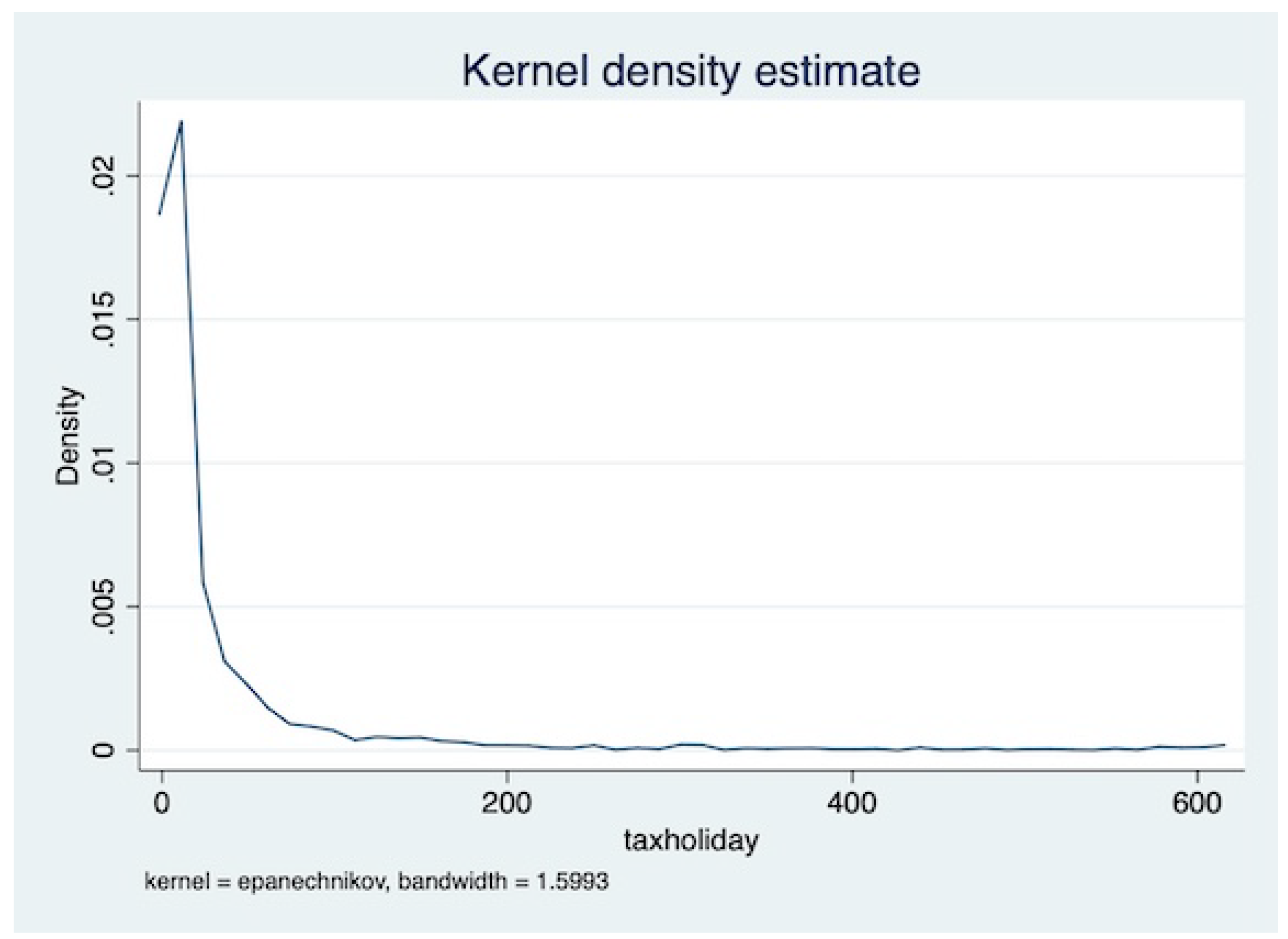
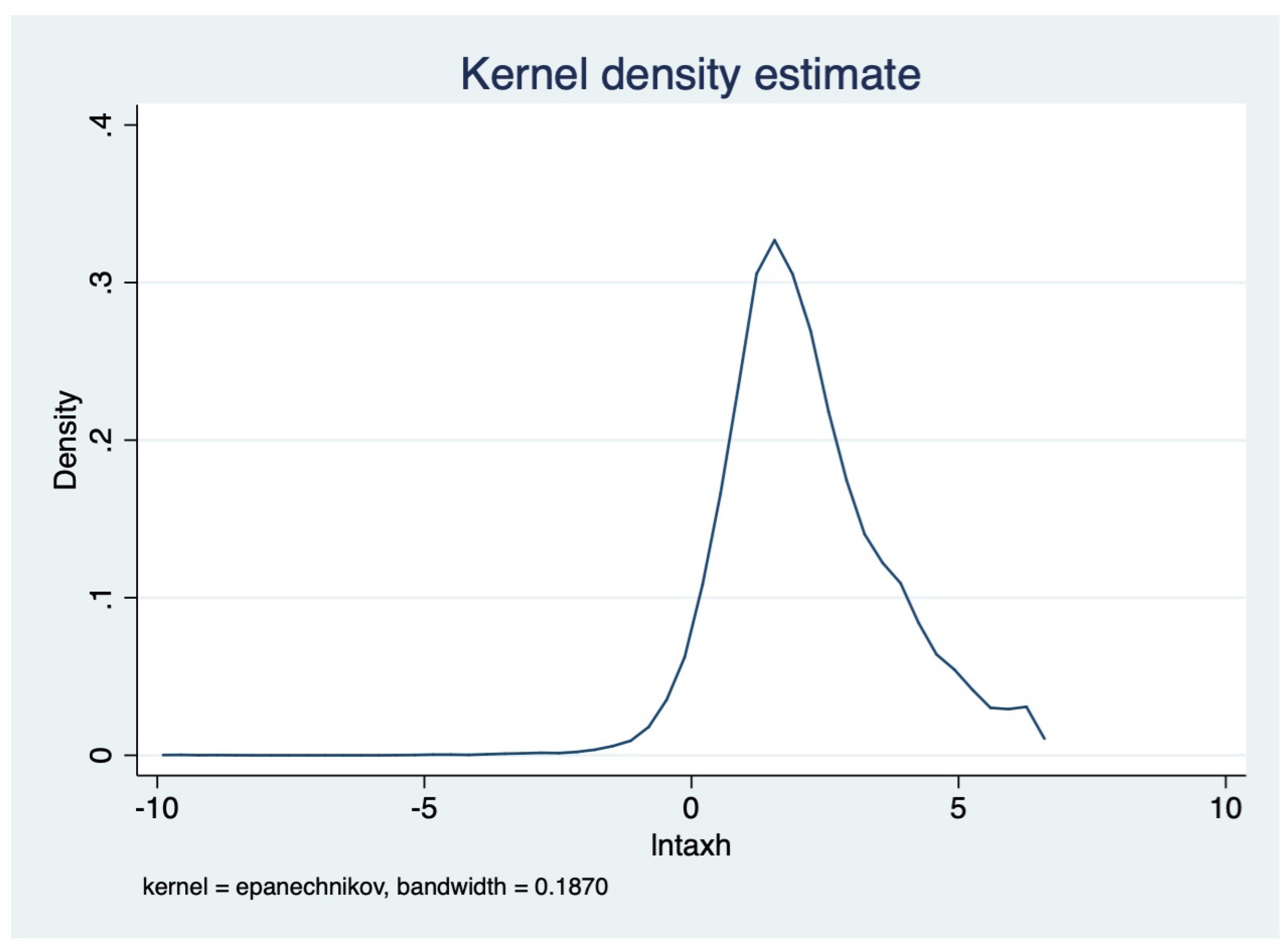
Since the distribution of tax holidays is quite skewed in the data, we use the natural log of tax holiday (denoted as Lntax) instead of its absolute value in order to avoid having outliers drive our results. The graphs showing the distribution of the tax holiday variable and its log are presented in Appendix C.

We estimate the following equation:

$$Lnta{x}_{ijt}={\theta }_1{Z}_{ijt}+{\theta }_2{S}_{jt}+\beta P{c}_{ijt}+f_i+D_t+{\epsilon }_{ijt}$$

(1)

where $Lnta{x}_{ijt}$ is the natural log of the amount of tax holiday firm i in industry j enjoys each year. $P{c}_{ijt}$ measures the level of political connectedness of each firm in a given year, $f_i$ is firm fixed effects and $D_t$ is time fixed effects. This way we account for any time-varying conditions that might affect productivity such as the state of the business cycle, as well as any firm characteristics that might affect productivity, so that the remaining variation in productivity must be accounted for only by firm-time-specific variables. $Z_{ijt}$ is a vector of firm-level control variables including state ownership indicator, export status and firm size (total number of workers) and $S_{jt}$ is a vector of industry-level control variables including number of firms and the level of intra-industry competition measured by the Lerner Index.

We expect a positive and statistically significant coefficient on $P{c}_{ijt}$ i.e., $\beta$, which means that the more politically connected a firm is, the more tax holiday it receives, controlling for firm heterogeneity and time-varying factors.

The level of political connectedness is represented by seven dummy variables already available in the dataset thanks to the innovative content of the questionnaire, part of which aims to understand firms’ social networks. For each of these variables, the value of 1 represents political connectedness and 0 represents the lack thereof. The seven binary proxies are listed and defined in

Table 4. Binary Variables Representing Political Connectedness.

Variable Name	Definition
Pc 1	Assistance at startup received from local authorities
Pc 2	Previous work status: whether manager was an employee of an SOE
Pc 3	Political Party Membership: whether manager was a Party member
Pc 4	Sales structure: % of goods sold to SOEs or local authorities of 30% or higher
Pc 5	% of procurement: % of goods procured from SOEs of 30% or higher
Pc 6	Selection of SOEs as suppliers or under direction by local authorities
Pc 7	Obtainment of services from SOEs

.

Here, the political party membership of the firm’s director or manager is represented by the third binary variable of political connection (Pc 3). In addition, the other six binary variables show other aspects of political connectedness, for example whether the firm received and assistance from local authorities at its early stage (Pc 1), whether the firm is directed by local authorities to select state-owned enterprises (SOEs) as its suppliers (Pc 6), or whether the firm’s sales or procurement are disproportionately with SOEs (Pc 4 and Pc 5).

This paper follows Williams (2019) in the recognition of the multi-dimensionality of otherwise omitted variables (in our case, political connectedness) as represented by these seven variables. This assertion on the multidimensional nature of political connectedness is supported by the values of correlations between these seven binary proxies as shown in

Table 5. Pairwise Correlations of Political Connection Variables.

	Pc 1	Pc 2	Pc 3	Pc 4	Pc 5	Pc 6	Pc 7
Pc 1	1
Pc 2	0.0136	1
Pc 3	0.0284 *	0.2468 *	1
Pc 4	0.0359 *	0.0743 *	0.0436 *	1
Pc 5	0.0262 *	0.0488 *	0.0240 *	0.1079 *	1
Pc 6	−0.0093	−0.0121	0.0081	0.0087	0.0304 *	1
Pc 7	0.0756 *	−0.0556 *	0.0173 *	0.0294 *	−0.0066	0.0226 *	1

Note: * p < 0.5.

. While most of these political connection variables are positively and significantly correlated with each other, the magnitudes of these correlations remain low, and some correlations are negative or insignificant, which suggests that these variables capture different aspects of political connectedness.

In the regression model, political connectedness is constructed in two ways: (i) as a vector of all seven of its dimensions, and (ii) collapsed into a sum of the seven dimensions for each firm in each year. The sum variable represents each firm’s degree of political connected in an aggregate sense, and would thus be meaningful for the assessment of how overall political connections interact with the allocation of tax subsidies.

Among the industry-level control variables, the Lerner Index represents the magnitude of importance of markups, defined as the difference between price and marginal cost with respect to the firm’s total value added. We follow Aghion et al. (2015) in first aggregating operating profits, capital costs and sales at the industry level then calculating the Lerner index as the ratio of operating profits less capital costs to sales. The value of Lerner index should vary between 0 and 1 with 0 reflecting perfect competition in which there should be no excess profits above capital costs. Therefore, the variable representing the degree of competition is defined as $(1-Lerne{r}_{-}Index)$ so that a greater value of this variable represents a greater level of competitiveness. We include this variable as Aghion et al. (2015) argue that it is important to control for the level of intra-industry competition when exploring the impact of industrial policy on firm performance.

Regarding tax holidays, we follow Aghion et al. (2015) in defining a firm as a recipient of a tax holiday in a year if that firm paid less than the statutory income tax rate. The amount of tax holiday for each firm is calculated as the difference between the amount of tax firm would have to pay given the statutory tax rates and the amount of tax they actually paid. For example, if the statutory income tax rate is 25% while a firm actually paid 20%, the tax holiday that firm enjoyed would be calculated by multiplying that firm’s operating profits by 5%. According to PricewaterhouseCoopers (2017), the corporate income tax rate in Vietnam was 25% until 2014.

Table 6. Vietnamese SMEs’ tax holidays between 2005 and 2015 (Unit: Million VND).

Amount of Tax Holiday				Year
(Million VND)	2004	2006	2008	2010	2012	2014	Total
0	256	75	93	109	2536	206	3275
>0 to 10	1736	1474	1477	1334	28	1512	7561
10 to 50	534	748	684	706	0	631	3303
50 to 100	126	147	173	171	0	131	748
100 to 300	122	121	154	143	0	93	633
>300	46	67	75	68	0	68	324
Total	2820	2632	2656	2531	2564	2641	15,844

shows the amount of tax holiday that Vietnamese SMEs enjoyed from 2005 to 2015. The first row of the table shows the number of firms which did not enjoy any tax incentive each year i.e., value of 0 for tax holiday.

As shown in Table 6, the number of firms that did not receive any tax holiday declined from 2004 to 2008 and then slightly increased in 2010 before reaching an unusually high number in 2012 and going back to similar level with pre-2012 period in 2014. A possible reason why there are as many as 2536 firms that did not enjoy any tax benefit in 2012 is that out of 2564 firms in the winsorized sample, 2435 firms reported making zero gross profit for that year. This shows that the SME sector of Vietnam was struggling after the global financial crisis and in particular in the years of 2011 and 2012—consistent with the information that 49,000 SMEs closed down in 2011.5 Even if we consider year 2012 as an outlier, in the robustness checks section we show that our results are robust to the exclusion of year 2012 from the dataset.

2.4. Impact of Industrial Support on Firm Productivity

Next, we explore the effects of industrial policy in the form of tax holidays on firm-level productivity. We expect that firms with political connections are less productive than other firms, and that the former would use tax benefits less productively than firms that are not politically connected. For this purpose, our regression includes the log of total factor productivity (TFP) as the dependent variable instead of tax holiday, and the log of tax holiday now as one of the explanatory variables:

$$lnTF{P}_{ijt}={\theta }_1{Z}_{ijt}+{\theta }_2{S}_{jt}+{\beta }_{1}Lnta{x}_{ijt}+{\beta }_{2}Tec{h}_{ijt}+f_i+D_t+{\epsilon }_{ijt}$$

(2)

$$\begin{array}{ccc}\hfill lnTF{P}_{ijt}=& & {\theta }_1{Z}_{ijt}+{\theta }_2{S}_{jt}+{\beta }_{1}Lnta{x}_{ijt}+{\beta }_{2}Tec{h}_{ijt}\hfill \\ & & +{\delta }_1{P}_{ijt}+{\delta }_2{P}_{ijt}\times Lnta{x}_{ijt}+f_i+D_t+{\epsilon }_{ijt}\hfill \end{array}$$

(3)

where $Lnta{x}_{ijt}$ is the log of tax holiday, $lnTF{P}_{ijt}$ is the log of TFP of firm i in industry j at time t, $Tec{h}_{ijt}$ is a dummy variable representing whether the firm received technical assistance from government at each time, $P_{ijt}$ is the vector of political connection indicator variables at the firm level including seven different binary variables drawn from the SME survey’s questionnaire. Similarly to Equation (1), $Z_{ijt}$ is a vector of firm-level controls and $S_{jt}$ is a vector of industry-level control variables, $f_i$ is firm fixed effects and $D_t$ is time fixed effects. The definition and measurement of TFP follows the Olley–Pakes method and is detailed in Appendix A.

We ran a Durbin–Wu–Hausman (Hausman) test to confirm the use of panel fixed-effects regression rather than random-effects regression on the main specification (2).6 In addition, we ran a Fisher-type unit root test for unbalanced panel dataset to confirm that the time series is stationary7 while it is also mentioned in Wooldridge (2010) that a unit root test is not necessary when the number of panel units is greater than the number of time periods.

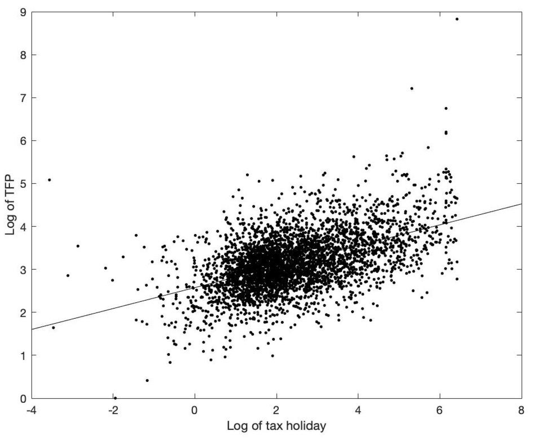
We predict a positive relationship between the firms’ average values of log of tax holiday and log of TFP over time, as shown in Figure 1 below of simple correlation with a simple linear trend line.

Equation (2) shows, through the coefficient of $Lnta{x}_{ijt}$, the impact of one percentage change in tax holiday on average firm-level productivity growth without accounting for political connections. Equation (3) features the political connection indicator variables and their interaction terms with tax holiday in addition to the existing explanatory variables already specified in Equation (2). As such, the coefficient of $Lnta{x}_{ijt}$ in Equation (3) shows the impact of tax holidays on the performance of firms that are not politically connected.

As mentioned above, we use the log of tax holiday instead of the amount of tax holiday because the distribution of tax holiday is quite skewed as shown in the kdensity graph in Figure A1 in Appendix C, so outliers could affect results. $Lnta{x}_{ijt}$ is also a better variable to use for the interpretation of its relationship with TFP since it shows the percentage change in the amount of tax holiday and not just the absolute amount itself.

2.5. Underlying Mechanism of Industrial Policy

Finally, we explore the potential mechanisms through which tax holidays might affect firm performance. We focus on two mechanisms as identified in the literature: (i) R&D intensity, and (ii) financing constraints, proxied by four technological variables. To do so, we re-run the regression of Equation (3) with additional interaction terms between log of tax holiday and the variables representing such characteristics. The specification is as follows:

$$\begin{array}{ccc}\hfill lnTF{P}_{ijt}=& & \theta Z_{ijt}+{\beta }_{1}Lnta{x}_{ijt}+{\beta }_{2}Tec{h}_{ijt}+{\delta }_1{P}_{ijt}+{\delta }_2{P}_{ijt}\times Lnta{x}_{ijt}+X_{jt}\hfill \\ & & +X_{jt}\times Lnta{x}_{ijt}+f_i+D_t+{\epsilon }_{ijt}\hfill \end{array}$$

(4)

where $X_{jt}$ is the variable representing either R&D intensity or financing constraints while other variables are as already defined. In the literature, several technological characteristics have been identified as proxies for financing constraints, including the level of depreciation, external finance dependence, asset fixity and investment lumpiness.

The reason we examine these variables is as follows. External finance dependence represents the extent to which a firm might be constrained financially due to its inherent need for external funds. On the other hand, other variables should be related to the firm’s ability to raise funds when needed. Specifically, according to Hart and Moore (1994), non-fixed assets are intangible and consequently less transferable and thus harder to use as collateral, rendering the firm more vulnerable to financing constraints. Faster depreciation rate of capital would also give its users less flexibility especially in using the capital as collateral on their loans. Finally, Samaniego (2010) proposes that investment lumpiness may also suggest that a substantial portion of a firm’s capital cannot be transferred without losing value, associating this technological characteristic to the value of specificity of capital and thus susceptibility to financing constraints.

Following Rajan and Zingales (1998), we use data on publicly traded firms in the United States to measure our technological variables. This is based on the assumption that the economic environment surrounding publicly traded firms in the United States economy is relatively frictionless, and thus can be used as a benchmark for measuring industry-level characteristics exogenous to the various frictions and conditions of developing economies such as Vietnam.

The measures for asset fixity ($FI{X}_{jt}$), capital depreciation rate ($DE{P}_{jt}$) and R&D intensity ($RN{D}_{jt}$) follow Samaniego and Sun (2015). Investment lumpiness ($LM{P}_{jt}$) is defined as in Ilyina and Samaniego (2011) as the “average number of investment spikes experienced by Compustat firms in a given industry” over a given period of time, in this case over every five year period. External finance dependence is as defined in Rajan and Zingales (1998): “the amount of desired investment that cannot be financed through internal cash flows generated by the same business”.

The formula to measure each variable is defined as follows:

(i)

Asset fixity is the ratio of fixed assets to total assets.

(ii)

Depreciation is measured as ratio of the value of depreciation to the value of property, plant and equipment.

(iii)

R&D intensity is measured as R&D expenditures over total capital expenditures.

(iv)

Investment lumpiness is defined as the average number of investment spikes experienced by firms in each industry while an investment spike is defined as an annual capital expenditure exceeding 30% of the firm’s fixed assets stock. $LM{P}_{jt}$ is thus a dummy variable that takes on the value of 1 if the ratio of annual capital expenditure to fixed assets is equal to or greater than 0.3. We take the average across all firms for each industry to represent the technological characteristic of investment lumpiness for the industry in a certain year.

(v)

A firm’s dependence on external finance is defined as capital expenditures minus cash flows from operations divided by capital expenditures. Cash flow from operations is calculated as the sum of cash flow from operations plus decreases in inventories, decreases in receivables, and increases in payables (Rajan and Zingales 1998).

All five technological variables are measured at the industry level using the Compustat database of firms in the United States. The years of the data taken from Compustat match the years of the survey in the Vietnamese SME dataset, namely every two years from 2004 to 2014. Each technological variable is calculated at the industry level by aggregating the value of each component over the time period for each firm, then taking the respective ratio for each firm, and using either the mean (for investment lumpiness, since this is a dummy variable) or median (for the other four variables in order to eliminate the impact of outliers) of each industry.

Since Compustat uses the North American Industry Classification System (NAICS) to map firms into industries while the Vietnamese SME database follows the International Standard Industrial Classification of All Economic Activities (ISIC) and the Vietnam Standard Industrial Classification 2007 (which is constructed based on ISIC Revision 4), we matched the industry codes across these different coding systems (at three-digit level) and merged the industry-level technological variables into the SME dataset.

The figures for five technological characteristics across different industries in the Compustat database are presented in

Table 7. Measurements of Technological Characteristics.

NAICS	Industry	FIX	EFD	DEP	LMP	RND
311	Food	0.292	−0.199	0.129	0.047	0
312	Beverage and Tobacco	0.245	−0.621	0.143	0.032	0
313	Textiles	0.367	−0.203	0.138	0.091	0.004
315	Apparel	0.133	−0.932	0.234	0.034	0
316	Leather and Allied Product	0.11	−0.825	0.24	0	0
321	Wood	0.448	−0.227	0.098	0	0
322	Paper	0.464	−0.327	0.112	0	0
323	Printing and Related	0.234	−0.96	0.227	0	0
324	Petroleum and Coal Product	0.497	−0.194	0.086	0.021	0
325	Chemical	0.067	1.813	0.282	0.029	0.363
326	Plastics and Rubber Products	0.298	0.077	0.157	0.029	0.004
327	Nonmetallic Mineral Product	0.387	0.171	0.114	0.079	0
331	Primary Metal	0.345	0.321	0.11	0.008	0
332	Fabricated Metal Product	0.232	−0.313	0.161	0.047	0.003
333	Machinery	0.137	0.702	0.212	0.026	0.024
334	Computer and Electronic Product	0.088	0.972	0.368	0.022	0.121
335	Electrical Equipment	0.16	1.343	0.204	0.028	0.026
336	Transportation Equipment	0.194	0.401	0.188	0.046	0.017
337	Furniture and Related Product	0.261	−0.246	0.163	0	0
339	Miscellaneous Manufacturing	0.101	1.432	0.318	0.016	0.061

Note: FIX (asset fixity), EFD (external finance dependence), DEP (depreciation), LMP (investment lumpiness), and RND (R&D intensity) are either the mean (for LMP) or median (for the others) value of all firms in an industry. The value of each variable for each firm by taking the respective ratio of its components which are aggregated over the period from 2004 to 2014 of Compustat data, matching the years of the Vietnamese SME survey. Industry codes follow the North American Industry Classification System.

. Since the distribution of R&D intensity is skewed with many zeros, we repeat the regression with R&D twice: first time by dropping the values of zeros and second time with bootstrapped errors in the robustness checks section.

Given our objective of identifying the impact of government support on firm-level performance, we restrict the sample to formal firms only because informal firms are not officially registered with the authorities and would thus be ineligible for formal government support. We define a firm as formal if the firm has either a tax code or a business registration license or an enterprise code number.

3. Results

3.1. Impact of Political Connections on the Allocation of Industrial Support

The regressions of tax holidays on political connectedness show a positive and significant relationship between political connections and tax subsidies.

Table 8. Effects of Political Connectedness (one proxy) on Tax Holiday Allocations.

	(1)
	Log of Tax Holiday
Total of All Political Binary Variables	0.0615 ***
	(0.0196)
Firm Size (Number of Employees)	0.00258 *
	(0.00147)
SOE Indicator	−0.0399
	(0.216)
Industry Competition Level	−1.168 ***
	(0.401)
Firm Fixed Effects	Yes
Year Dummies	Yes
Number of observations	9259
R${}^2$	0.0849

Robust standard errors in parentheses, clustered at the firm level. * p < 0.1, ** p < 0.05, *** p < 0.01.

shows the results with political connectedness being represented by the sum of all political dummies, while

Table 9. Effects of Political Connections (seven proxies) on Tax Holiday Allocations.

	(1)
	Log of Tax Holiday
Pc 1 (Assistance at startup)	0.100 *
	(0.0603)
Pc 2 (Previous work status of owner/manager)	0.0330
	(0.0399)
Pc 3 (Political party membership of owner/manager)	0.0250
	(0.0738)
Pc 4 (Sales structure)	0.107 **
	(0.0534)
Pc 5 (Procurement structure)	0.0428
	(0.0440)
Pc 6 (Selection of SOEs as supplier)	0.605
	(0.429)
Pc 7 (Obtainment of services from SOEs)	0.0808
	(0.0513)
Firm Size (Number of Employees)	0.00260 *
	(0.00147)
SOE Indicator	−0.0437
	(0.208)
Industry Competition Level	−1.177 ***
	(0.400)
Industry Size (Number of Firms)	0.000994
	(0.00127)
Year Fixed Effects	Yes
Number of observations	9259
R${}^2$	0.0856

Robust standard errors in parentheses, clustered at the firm level. * p < 0.1, ** p < 0.05, *** p < 0.01.

shows the results of the regression using all binary proxies of political connections. While the coefficient on the sum of the binary variables is significant and positive, the coefficients on Pc 1 and Pc 4 in Table 9 are significant and positive, whereas the others are positive but not significant. To sum up, we find that some forms of political connections do appear associated with better access to tax holidays.

3.2. Impact of Industrial Policy and Underlying Mechanism

Table 10. Effects of Tax Holiday on Firm Productivity.

	(1)	(2)
	TFP_OP	TFP_OP
Log of Tax Holiday	0.253 ***	0.275 ***
	(0.0149)	(0.0162)
Technical Assistance (Dummy)	−0.0647	−0.0643
	(0.0616)	(0.0604)
Firm Size (Number of Employees)	−0.00216 ***	−0.00210 ***
	(0.000578)	(0.000565)
SOE indicator	0.241	0.257
	(0.241)	(0.251)
Industry Size (Number of Firms)	0.00153 *	0.00154 *
	(0.000835)	(0.000843)
Industry Competition Level	0.115	0.127
	(0.235)	(0.237)
Pc 1		−0.0559
		(0.0822)
Pc 2		0.0543
		(0.0521)
Pc 3		−0.111
		(0.0750)
Pc 4		0.0775
		(0.0771)
Pc 5		0.0517
		(0.0792)
Pc 6		−0.835
		(0.626)
Pc 7		0.0634
		(0.0472)
Interaction Term Pc 1 & Log of Tax Holiday		0.0528 *
		(0.0276)
Interaction Term Pc 2 & Log of Tax Holiday		−0.0241
		(0.0172)
Interaction Term Pc 3 & Log of Tax Holiday		0.00256
		(0.0225)
Interaction Term Pc 4 & Log of Tax Holiday		−0.0205
		(0.0238)
Interaction Term Pc 5 & Log of Tax Holiday		−0.0398
		(0.0253)
Interaction Term Pc 6 & Log of Tax Holiday		0.219
		(0.229)
Interaction Term Pc 7 & Log of Tax Holiday		−0.0155
		(0.0129)
Number of observations	8583	8513
R${}^2$	0.183	0.187

Robust standard errors in parentheses, clustered at the firm level. All regressions include firm fixed effects and year dummies. * p < 0.1, ** p < 0.05, *** p < 0.01.

below shows the results of the fixed-effects panel regressions for each of the two specifications. Model specification (2) controls for firm-level variables without controlling for political connectedness. Model specification (3) includes the seven binary proxies representing political connectedness and the interaction terms between the political connection binary proxies and the tax holiday variable.

Table 11. Mechanism Testing with Five Technological Characteristics.

	(1)	(2)	(3)	(4)	(5)
	TFP_OP	TFP_OP	TFP_OP	TFP_OP	TFP_OP
Log of Tax Holiday	0.273 ***	0.280 ***	0.251 ***	0.274 ***	0.285 ***
	(0.0163)	(0.0155)	(0.0385)	(0.0207)	(0.0350)
RND	−0.358
	(0.363)
Interaction Term RND & Log of Tax Holiday	0.267 **
	(0.135)
Technical Assistance (Dummy)	−0.0663	−0.0654	−0.0634	−0.0643	−0.0642
	(0.0602)	(0.0604)	(0.0605)	(0.0603)	(0.0604)
Firm Size (Number of Employees)	−0.00210 ***	−0.00210 ***	−0.00211 ***	−0.00210 ***	−0.00211 ***
	(0.000563)	(0.000565)	(0.000570)	(0.000566)	(0.000566)
SOE Indicator	0.270	0.259	0.254	0.256	0.254
	(0.254)	(0.251)	(0.251)	(0.251)	(0.251)
Industry Size (Number of Firms)	0.00164 *	0.00166 **	0.00159 *	0.00158 *	0.00156 *
	(0.000847)	(0.000831)	(0.000845)	(0.000840)	(0.000854)
Industry Competition Level	0.121	0.115	0.128	0.139	0.128
	(0.237)	(0.236)	(0.238)	(0.238)	(0.238)
Pc 1	−0.0572	−0.0580	−0.0531	−0.0549	−0.0556
	(0.0821)	(0.0821)	(0.0823)	(0.0821)	(0.0822)
Pc 2	0.0554	0.0559	0.0548	0.0553	0.0544
	(0.0520)	(0.0518)	(0.0519)	(0.0520)	(0.0520)
Pc 3	−0.108	−0.111	−0.112	−0.111	−0.112
	(0.0749)	(0.0752)	(0.0754)	(0.0753)	(0.0753)
Pc 4	0.0837	0.0872	0.0769	0.0751	0.0764
	(0.0767)	(0.0769)	(0.0782)	(0.0766)	(0.0778)
Pc 5	0.0505	0.0522	0.0519	0.0518	0.0524
	(0.0791)	(0.0787)	(0.0786)	(0.0792)	(0.0791)
Pc 6	−0.842	−0.809	−0.822	−0.849	−0.831
	(0.627)	(0.625)	(0.627)	(0.634)	(0.626)
Pc 7	0.0628	0.0617	0.0607	0.0635	0.0625
	(0.0471)	(0.0469)	(0.0471)	(0.0472)	(0.0471)
Interaction Term Pc 1 & Log of Tax Holiday	0.0534 *	0.0541 *	0.0521 *	0.0530 *	0.0528 *
	(0.0275)	(0.0276)	(0.0276)	(0.0275)	(0.0276)
Interaction Term Pc 2 & Log of Tax Holiday	−0.0247	−0.0250	−0.0242	−0.0243	−0.0241
	(0.0171)	(0.0171)	(0.0171)	(0.0171)	(0.0172)
Interaction Term Pc 3 & Log of Tax Holiday	0.000595	0.000980	0.00253	0.00223	0.00273
	(0.0225)	(0.0226)	(0.0226)	(0.0225)	(0.0226)
Interaction Term Pc 4 & Log of Tax Holiday	−0.0222	−0.0234	−0.0206	−0.0198	−0.0202
	(0.0236)	(0.0237)	(0.0241)	(0.0237)	(0.0240)
Interaction Term Pc 5 & Log of Tax Holiday	−0.0389	−0.0395	−0.0402	−0.0399	−0.0401
	(0.0253)	(0.0251)	(0.0251)	(0.0253)	(0.0253)
Interaction Term Pc 6 & Log of Tax Holiday	0.221	0.202	0.215	0.226	0.217
	(0.229)	(0.230)	(0.227)	(0.232)	(0.228)
Interaction Term Pc 7 & Log of Tax Holiday	−0.0155	−0.0155	−0.0146	−0.0155	−0.0153
	(0.0128)	(0.0127)	(0.0127)	(0.0129)	(0.0127)
EFD		−0.0569
		(0.0579)
Interaction Term EFD & Log of Tax Holiday		0.0285
FIX			−0.213
			(0.317)
Interaction Term FIX & Log of Tax Holiday			0.0876
			(0.116)
LMP				0.970
				(1.289)
Interaction Term LMP & Log of Tax Holiday				0.0242
				(0.411)
DEP					0.179
					(0.545)
Interaction Term DEP & Log of Tax Holiday					−0.0623
					(0.215)
Year Fixed Effects	Yes	Yes	Yes	Yes	Yes
R${}^2$	0.188	0.188	0.188	0.188	0.187

Robust standard errors in parentheses, clustered at the firm level All regressions include firm fixed effects and year dummies. * p < 0.1, ** p < 0.05, *** p < 0.01.

shows the tests for potential underlying mechanisms with each of the five technological measures at the industry level and its interaction term with the tax holiday variable added to model specification (3).

It can be seen from the results that tax benefits lead to an increase in firm-level productivity as the coefficients on the log of tax holiday are positive and significant in both specifications. The coefficient of 0.253 in model specification (2) implies that an increase in tax holiday by 1% is associated with an increase of 0.253% in firm-level TFP. This coefficient increases to 0.275 in model specification (3), showing that when political connectedness is controlled for, tax holidays have a greater effect on firm productivity, and that firms without political connections would be more productive with tax holidays than firms that are politically connected. In addition, the political connection variables are also found to be jointly significant.

Observe that not all the political connections interactions have the same sign. While the preponderance of the literature finds that political connections weaken any positive impact of industrial support on firm outcomes, the fact that we find this is not necessarily always the case is consistent with Ouyang and Zhang (2019). This underlines the importance of using several proxies for political connections—both for adequately conditioning on political connections, and for adequately identifying their impact.

The positive and significant value of the coefficient of the interaction term between R&D intensity and tax holiday in Table 11 indicates that industries that are more R&D intensive would be more productive with tax subsidies from the government. Lack of significant results on the other technological variables representing financing constraints indicate that relieving financing constraints is not the main way industrial policy affects firm-level productivity. Later we study government technical assistance to firms and tariff rates as alternative instruments of industrial policy, finding they do not seem to have a significant impact on firm performance.

We conclude that industrial support in the form of tax holidays increases productivity growth, particularly in R&D intensive industries, and particularly among firms that are not politically connected. We also find no evidence that financing constraints play a role in these results.

3.3. Robustness Checks

We check the robustness of the results with respect to (i) the setting of tariff rates at the industry level as an alternative proxy of industrial policy, and (ii) a combination of “stickier” political connection variables to address endogeneity concerns. Additional robustness checks are performed in Appendix D with regard to (i) alternative measures of TFP i.e., TFP calculated using OLS Fixed Effects (FE) and the Levinsohn–Petrin methods, (ii) alternative underlying mechanisms i.e., the mechanism proposed by Aghion et al. (2015) where industrial policy works through fostering competition measured by the Herfindahl index representing the dispersion of subsidies within each industry, (iii) the consideration of the skewed distribution of R&D intensity by repeating the regression either by dropping values of zero or with bootstrapped errors, (iv) excluding 2012 to make sure the results hold without major outliers, (v) subsamples of firms of different sizes, and (vi) post-estimation tests.

3.3.1. Use of Tariff Rates as Industrial Policy

In the industrial policy literature, tariffs are also considered a measure of industrial policy, one that can be affected by political connections: see Grossman and Helpman (1994) and Goldberg and Maggi (1999). A higher tariff rate signifies protectionism against foreign competition. A low tariff rate, however, means cheaper imports of inputs for production. Therefore, it is not clear what impact tariff rates have on firm performance. We test this industrial policy measure by including tariff rates at the industry level instead of tax holidays as the proxy for industrial policy in the regression model.

We obtained tariff data from the World Bank Integrated Trade Solution (WITS) platform for corresponding years and calculated tariff rates imposed by Vietnam at the industry level. The tariff rate in use is the average maximum input tariff rate that the Vietnamese government set for countries with Most Favored Nations status. The tariff rates by industry from 2004 to 2014 are shown in

Table 12. Vietnam’s Average Tariff Rates by Manufacturing Industry from 2004 to 2014 (%).

Sector	2004	2006	2008	2010	2012	2014
Primary production/Agriculture	15.2	15.3	12.6	10.1	9.8	10.1
Food and beverages	32.8	32.6	24.5	21.5	20.3	20.7
Tobacco	65.0	65.0	82.5	80.0	78.6	80.0
Textiles	32.8	32.8	10.1	10.0	10.0	10.0
Apparel	48.4	48.4	20.4	20.1	19.8	19.8
Leather	29.0	29.0	23.0	20.2	18.4	18.4
Wood	12.9	12.9	11.1	9.1	8.6	8.4
Paper	20.1	20.1	16.9	14.4	12.8	12.7
Publishing and printing	21.9	21.9	16.5	13.6	12.7	12.3
Refined petroleum etc.	5.6	5.6	3.4	4.7	3.7	4.6
Chemical products etc.	4.4	4.4	3.6	3.0	2.6	2.6
Rubber	18.5	18.5	16.4	14.5	13.2	12.8
Non-metallic mineral products	24.4	24.4	21.3	20.0	19.0	19.1
Basic metals	4.2	4.2	2.4	2.7	2.5	2.9
Fabricated metal products	18.8	18.8	16.4	15.2	14.5	14.7
Electronic machinery, computers, radio, tv, etc.	10.7	10.7	8.1	7.1	6.2	6.3
Motor vehicles etc.	53.8	53.9	36.7	40.1	35.7	34.3
Other transport equipment	15.4	15.4	14.3	13.4	12.3	12.3
Furniture, jewellery, toys, music equipment etc.	17.2	17.2	13.9	12.1	11.5	11.6
Services	8.5	8.3	7.4	6.6	6.2	6.4

.

When we include the measure of tariffs at the industry level instead of tax holiday in the right hand side of the regressions, we do not obtain significant results for the coefficients on the tariff variable, which suggests that preferential treatment in terms of tariff rates at the industry level does not seem to have an impact on firm productivity. These results are shown in

Table 13. Robustness Checks with Tariff Rates at the Industry Level as Additional Policy Measure.

	(1)
	TFP_OP
Tariff	0.000264
	(0.000640)
Technical Assistance (Dummy)	0.00677
	(0.0571)
Firm Size (Number of Employees)	−0.00142 ***
	(0.000220)
SOE Indicator	0.152
	(0.176)
Industry Size (Number of Firms)	0.000987
	(0.000707)
Industry Competition Level	−0.163
	(0.260)
Firm Fixed Effects	Yes
Year Dummies	Yes
Number of observations	10955
R${}^2$	0.0194

Robust standard errors in parentheses, clustered at the firm level. * p < 0.1, ** p < 0.05, *** p < 0.01.

below.

3.3.2. Combination of “Stickier” Political Connection Variables

As the level of firm productivity is controlled for with the inclusion of firms’ fixed effects, an additional robustness check is conducted to verify that any reverse causality between political connection and firm productivity e.g., firms seek to change their level of political connectedness in response to their productivity shocks, is not a significant concern. We thus select the political connection variables that are less easy to adjust over time i.e., “stickier” or less sensitive to productivity shocks in other words, and rerun the regressions with those connection variables only. The variables we select are those related to the firms’ links to an SOE (variables 4, 5 and 7). The coefficient on tax holiday remains stable with these alternative regressions, which confirms the validity of the identification strategy as shown in

Table 14. Robustness Checks with “Stickier” Political Connection Variables.

	(1)
	TFP_OP
Log of Tax Holiday	0.271 ***
	(0.0157)
Technical Assistance (Dummy)	−0.0700
	(0.0618)
Firm Size (Number of Employees)	−0.00216 ***
	(0.000570)
SOE indicator	0.230
	(0.250)
Industry size (Number of Firms)	0.00155 *
	(0.000835)
Industry Competition Level	0.136
	(0.237)
Pc 4 (Sales structure)	0.0759
	(0.0778)
Pc 5 (Procurement structure)	0.0645
	(0.0780)
Pc 7 (Obtainment of services from SOEs)	0.0427
	(0.0472)
Interaction term Pc 4 & Tax Holiday	−0.0192
	(0.0240)
Interaction term Pc 5 & Tax Holiday	−0.0450 *
	(0.0249)
Interaction term Pc 7 & Tax Holiday	−0.00885
	(0.0129)
Firm Fixed Effects	Yes
Year Dummies	Yes
Number of observations	8572
R${}^2$	0.186

Robust standard errors in parentheses, clustered at the firm level. * p < 0.1, ** p < 0.05, *** p < 0.01.

below.

4. Discussion

In this section, we present an extension of the Howitt (1999) framework, generalized to allow for many heterogeneous industries.8 In the model, industries vary in terms of their market size and, as in Schmookler (1966), this leads R&D intensity to vary endogenously across industries, because larger product markets encourage innovation by offering greater returns to successful innovators. Some empirical studies of specific products or industries find some evidence of a demand-innovation link—for example, Newell et al. (1999), Popp (2002) and Acemoglu and Linn (2004). These findings underline the importance of demand in providing incentives for R&D. There is also broad aggregate empirical support for creative-destruction style models, see for example Ha and Howitt (2007), Madsen (2008) or Ang and Madsen (2011). In particular, Ang and Madsen (2011) find that this class of model best explains the experience of the East Asian “miracle” economies. An interpretation of our paper is that it provides new cross-sectional support for this kind of model.

In the model, there is a quality ladder that firms may approach by performing R&D. Thus, technology adoption requires investment, consistent with the findings in Cohen and Levinthal (1990) and Griffith et al. (2004). As a spillover, this absorptive R&D also reveals the path to adopting further technologies in the future.

4.1. Household Preferences

Time is continuous, and there is a $\left[0,1\right]$ continuum of dynasties, each of mass $L_t=L_0{e}^{g_L^t}$. We assume that the rate of population growth $g_L^t>0$ is exogenous.

There are $I\in \mathbb{N}$ types of final good in the economy, each produced by a separate industry. There exists in turn $\left[0,Q_{it}\right]$ continuum of varieties of each good $i\le I$. Let $c_{hit}$ be consumption of variety h of good i at date t. Dynastic preferences over consumption $c_t$ are:

$${\int }_0^{\infty }{e}^{-rt}{L}_{t}u\left(c_t\right)dt$$

(5)

where u is the instantaneous utility function and r is the discount rate. Consumption $c_t$ is an aggregate of the agent’s consumption $c_{it}$ of each good $i\le I$, which is in turn an aggregate over the varieties $h\in \left[0,Q_{it}\right]$:

$$c_t=\prod _{i=1}^I{\left(\frac{c_{it}}{{\omega }_i}\right)}^{{\omega }_i},c_{it}={\int }_0^{Q_{it}}{c}_{hit}dh,i\in \left\{1,\cdots ,I\right\}$$

(6)

where the preference parameter ${\omega }_i$ is the equilibrium share of expenditure devoted to good i, which will be a key determinant of equilibrium R&D intensity. Each agent is also endowed with one unit of labor that may be spent working in production, or in research, as described below. In either case, it earns the competitive wage $w_t$.

Their budget constraint is

$$\sum _{i=1}^I{q}_{it}{\int }_0^{Q_{it}}{c}_{iht}dh\le {\Pi }_t+w_t\left(L_t-R_t\right)+T_t\equiv L_t{S}_t$$

(7)

where we have used the fact that all varieties h of any good i are perfect substitutes, so they all command the same price $q_{it}$ in equilibrium.9 Here ${\Pi }_t$ equals after-tax profits from various sources, and $T_t$ is a lump sum transfer, both in terms of the numeraire. $R_t$, to be expanded upon later, is the use of labor in research rather than goods’ production. Also $w_t$ is the competitive wage. We set $w_t=1$ so labor is the numeraire, and define $S_t$ as income per capita, in terms of the numeraire.

4.2. Final Goods

Each variety h of good i is supplied by a monopolist (below the variety index h is suppressed for simplicity). Each monopolist holds a patent on the technology for producing that variety, indexed by the date v at which the innovation took place (its vintage). At any date t, the production function for any given variety of good i for this monopolist is $y_{it}\left(v\right)=A_{iv}{x}_{it}^{\alpha }$, where $y_{it}\left(v\right)$ is output, $x_{it}$ is input of a variety-specific intermediate and $A_{iv}$ is the productivity of the monopolist’s technology. The monopolist solves:

$$max\left\{q_{it}{A}_{iv}{x}_{it}^{\alpha }-p_{it}{x}_{it}\right\}\left(1-\tau \right)$$

(8)

where $q_{it}$ is the price of good i and $p_{it}$ is the marginal cost of the intermediate. Here $\tau$ is the tax rate on earnings.

The solution to (8) implies:

$$p_{it}\left(x_{it}\right)=\alpha q_{iv}{A}_{it}{x}_{it}^{\alpha -1}$$

(9)

4.3. Intermediate Goods

A patent-holding monopolist produces the intermediate $x_{it}$ using labor. The monopolist solves the static profit maximization problem:

$$\underset{x_{it}}{max}\left\{p_{it}\left(x_{it}\right)x_{it}-w_t{x}_{it}\right\}\left(1-\tau \right),$$

(10)

where the inverse demand curve $p_{it}\left(·\right)$ is given by (9), so this becomes

$$\left(1-\tau \right)\underset{x_{it}}{max}\left\{\alpha q_{it}{A}_{iv}{x}_{it}^{\alpha }-w_t{x}_{it}\right\}.$$

The solution to this problem is

$$x_i\left(v,t\right)={\left(\frac{{\alpha }^2{q}_{it}{A}_{iv}}{w_t}\right)}^{\frac{1}{1-\alpha }},$$

(11)

so that output of the variety equals $y_{it}\left(v\right)\equiv A_{iv}{\left(\frac{{\alpha }^2{q}_{it}{A}_{iv}}{w_t}\right)}^{\frac{\alpha }{1-\alpha }}$. Thus, pre-tax profits for a patent holder are:

$${\pi }_{ir}\left(v,t\right)\equiv {\left(\frac{q_{it}{A}_{iv}}{w_t^{\alpha }}\right)}^{\frac{1}{1-\alpha }}\pi$$

(12)

where $\pi \equiv \left[\alpha \times {\alpha }^{\frac{2\alpha }{1-\alpha }}-{\alpha }^{\frac{2}{1-\alpha }}\right]$. This also implies that, if ${\pi }_{ip}\left(v,t\right)$ are the pre-tax profits of the final good producers, then:

$${\pi }_{ip}\left(v,t\right)=\left(1-\alpha \right){\left(q_{it}{A}_{iv}\right)}^{\frac{1}{1-\alpha }}{\left(\frac{{\alpha }^2}{w_t}\right)}^{\frac{\alpha }{1-\alpha }}$$

(13)

4.4. Vertical Innovation

Agents may invest in R&D in order to uncover the technology to produce the intermediate good corresponding to a variety of good i at the current frontier productivity $A_{it}^{max}$, which grows at rate $g_i$. If an agent dedicates $N_{it}$ units of labor to R&D in industry i, she harvests innovations at rate $\lambda N_{it}$. It will be convenient to define ${\overline{N}}_{it}$ as the total resources devoted to vertical innovation in industry i, and ${\overline{n}}_{it}=\frac{{\overline{N}}_{it}}{Q_{it}}$ as the amount of vertical R&D per variety of good i. Since one firm produces each variety it is also interpretable as the vertical R&D per firm in industry i.

Growth in the frontier technology $A_{it}^{max}$ is determined by spillovers from research. If the total amount of R&D in industry i is $N_{it}$, then the flow of new technologies for producing good i is

$${\dot{A}}_{it}^{max}=\frac{\lambda {\overline{N}}_{it}{A}_{it}^{max}}{Q_{it}}\sigma .$$

(14)

This function assumes that new technologies depend on the rate of innovations $\lambda {\overline{N}}_{it}$. The parameter $\sigma$ indicates the intensity of technological knowledge spillovers. The numerator $Q_{it}$ reflects the idea that research effort is dissipated across varieties $Q_{it}$, the key mechanism of the Howitt (1999) model for avoiding scale effects. Finally, the spillover function (14) depends positively on the current frontier level $A_{it}^{max}$, reflecting a “standing on shoulders” effect for which Ngai and Samaniego (2011) among others find evidence.

As a result, the growth rate of the technology frontier in industry i is:

$$g_i\equiv \frac{{\dot{A}}_{it}^{max}}{A_{it}^{max}}=\frac{\lambda {\overline{N}}_{it}}{Q_{it}}\sigma =\lambda {\overline{n}}_{it}\sigma .$$

(15)

A successful innovator replaces the incumbent monopolist, and earns expected discounted profits ${\tilde{V}}_{it}$ where

$${\tilde{V}}_{it}={\int }_t^{\infty }{e}^{-\left(r+\lambda {\overline{n}}_{is}\right)s}\left(1-\tau \right){\pi }_{is}\left(t,s\right)ds.$$

(16)

The exponent $\lambda {\overline{n}}_{is}$ reflects the fact that, in expectation, future researchers may in turn displace the innovator. This displacement rate is $\lambda \frac{{\overline{N}}_{is}}{Q_{is}}$, because it is increased by the research effort of others, and dissipated by there being more varieties across which future innovation might occur.

Notice that $\tau$ enters ${\tilde{V}}_{it}$. This is because taxes reduce the potential earnings of successful researchers. It will be convenient to define $V_{it}\equiv {\tilde{V}}_{it}/\left(1-\tau \right)$, which does not depend on any taxes.

Thus, we have that the marginal return to spending a unit of labor on research in industry i is $\lambda V_{it}\left(1-\tau \right)$. The marginal cost is $w_t$, the price of labor. These must be equal when R&D input is optimal:

$$\lambda \left(1-\tau \right)V_{it}=w_t.$$

(17)

Combining (12), (16) and (17), optimal vertical R&D choices satisfy:

$$w_t=\left(1-\tau \right)\lambda {\int }_0^{\infty }{e}^{-\left(r+\lambda {\overline{n}}_{is}\right)s}\left[{\left(\frac{q_{is}{A}_{it}^{max}}{w_s^{\alpha }}\right)}^{\frac{1}{1-\alpha }}\pi \right]ds.$$

(18)

4.5. Horizontal Innovation

Agents may also invest in producing new varieties of any good i. If agents invest $M_{it}$ units of labor in the production of new varieties in industry i, the flow of new varieties is given by:

$${\dot{Q}}_{it}=\mathsf{\Psi }\left(M_{it},Q_{it}\right)$$

(19)

where $\mathsf{\Psi }$ is increasing and homogeneous of degree one. This structure assumes that having more varieties aids the production of new varieties, another “standing-on-shoulders” effect.

Let $h_{it}=M_{it}/Q_{it}$, the horizontal R&D per firm, and define $\psi \left(·\right)\equiv \mathsf{\Psi }\left(·,1\right)$. We can rewrite (19) as:

$$\begin{array}{ccc}\hfill {\dot{Q}}_{it}& =& \mathsf{\Psi }\left(h_{it},1\right)Q_{it}\hfill \\ & =& \psi \left(h_{it}\right)Q_{it}.\hfill \end{array}$$

A horizontal innovation in industry i draws its productivity level $A_{iv}$ from the existing distribution in industry i. It is straightforward to show that the expected discounted profits of a monopolist with technology of vintage v is ${\left(\frac{A_{iv}}{A_{it}^{max}}\right)}^{\frac{1}{1-\alpha }}{\tilde{V}}_t$. As a result, the expected profits from a horizontal innovation are:

$$E\left[{\left(\frac{A_{iv}}{A_{it}^{max}}\right)}^{\frac{1}{1-\alpha }}\right]{\tilde{V}}_t$$

where the expectation is taken over the distribution of $A_{iv}$ at date t. If $f_i\left(v,t\right)$ is the distribution of firms over v at date t, then this expectation becomes ${\int }_{-\infty }^t{\left(\frac{A_{iv}}{A_{it}^{max}}\right)}^{\frac{1}{1-\alpha }}{f}_i\left(v,t\right)dv$.

For horizontal R&D allocations to be optimal, the marginal cost of R&D must equal this expression, times the marginal effect of an additional unit of labor devoted to production of new varieties in industry i. The marginal flow of new varieties is ${\mathsf{\Psi }}_1\left(M_{it},Q_{it}\right)=\frac{d\left[\mathsf{\Psi }\left(\frac{M_{it}}{Q_{it}},1\right)Q_{it}\right]}{d{M}_{it}}={\mathsf{\Psi }}_1\left(\frac{M_{it}}{Q_{it}},1\right)={\psi }^{\prime }\left(h_{it}\right)$. Thus, optimal horizontal R&D allocations satisfy:10

$$w_t={\psi }^{\prime }\left(h_{it}\right).E\left[{\left(\frac{A_{iv}}{A_{it}^{max}}\right)}^{\frac{1}{1-\alpha }}\right]V_t\left(1-\tau \right).$$

(20)

4.6. Government

The government collects taxes and redistributes them as a lump sum transfer $T_t$, balancing its budget every period. If $f_i\left(v,t\right)$ is the distribution of firms over v at date t industry i, the corresponding measure is $Q_{it}{f}_i\left(v,t\right)$, and the balanced budget condition becomes:

$$T_t=\tau \sum _i{Q}_{it}{\int }_{-\infty }^t{\pi }_{ip}\left(v,t\right)f_i\left(v,t\right)dv+\tau \sum _i{Q}_{it}{\int }_{-\infty }^t{\pi }_{ir}\left(v,t\right)f_i\left(v,t\right)dv$$

This notation also allows us to define after-tax profits ${\Pi }_t:$

$${\Pi }_t=\left(1-\tau \right)\sum _i{Q}_{it}{\int }_{-\infty }^t{\pi }_{ip}\left(v,t\right)f_i\left(v,t\right)dv+\left(1-\tau \right)\sum _i{Q}_{it}{\int }_{-\infty }^t{\pi }_{ir}\left(v,t\right)f_i\left(v,t\right)dv.$$

This means that in equilibrium the household’s balanced budget condition must satisfy:

$$L_t{S}_t=w_t\left(L_t-\sum _i{N}_{it}-\sum _i{M}_{it}\right)+\sum _i{Q}_{it}{\int }_{-\infty }^t{\pi }_{ip}\left(v,t\right)f_i\left(v,t\right)dv+\sum _i{Q}_{it}{\int }_{-\infty }^t{\pi }_{ir}\left(v,t\right)f_i\left(v,t\right)dv.$$

4.7. Stationary Equilibrium

Definition 1.

A stationary equilibrium (or “equilibrium” henceforth) is a set of initial conditions ${\left\{Q_{i0},f_i\left(·,0\right)\right\}}_{i\le I}$ and allocations such that households are optimizing based on their budget constraints, the government balances its budget every period, $n_{it}=n_i$ at all dates t and $h_{it}=h_i$ at all dates.

Proposition 1.

Equilibrium exists and is unique.

Proof. 

See Appendix B. □

Definition 2.

Research intensity in industry i at date t is defined as research expenditure per firm in industry i,11

$$\begin{array}{ccc}\hfill {\rho }_{it}& =& \frac{\left(N_{it}+M_{it}\right)w_t}{Q_{it}}\hfill \\ & =& \left(n_{it}+h_{it}\right)w_t.\hfill \end{array}$$

Set labor as the numeraire so $w_t=1$ at all dates. In Appendix B we show that, in equilibrium,

$$n_{it}={\overline{n}}_i=max\left\{0,\frac{\left(1-\tau \right)\pi {\omega }_{i}S{L}_0}{{\alpha }^{\frac{2\alpha }{1-\alpha }}{Q}_{i0}}-\frac{r}{\lambda \left(1+\frac{1}{1-\alpha }\sigma \right)}\right\}.$$

(21)

which does not depend on time. In addition, we are able to show that $h_{it}$ does not vary across time nor across industries. It follows that variation in research intensity depends only on ${\overline{n}}_i$, so that:

Proposition 2.

In equilibrium,

(i) 

research intensity is constant over time in all industries—${\rho }_{it}={\overline{\rho }}_i$;

(ii) 

equilibrium research intensity is positive in at least one industry, provided r is sufficiently small;

(iii) 

equilibrium research intensity ${\overline{\rho }}_i$ is increasing in ${\omega }_i/Q_{i0}$–strictly among industries $i:$ ${\overline{\rho }}_i>0$.

Proposition 2 tells us that, in our multi-industry environment, the key determinant of research intensity is market size, normalized by the initial number of varieties. This is a twist on the original idea of Schmookler (1966): the market size that is available to an innovator depends both on the preference parameter ${\omega }_i$ and on the intensity of competition in that market—given initially by $Q_{i0}$—which dissipates the returns to R&D.

Proposition 2 might also appear to suggest that a larger economy (i.e., with a larger initial value of $L_0$) might have higher R&D intensity and thus productivity growth—even if the model structure avoids the “scale effects” problem that economies with a growing population grow at an accelerating rate. However it is worth underlining that the model as it stands takes $L_0$ and ${\left\{Q_{i0}\right\}}_i$ as given and independent variables—it does not provide a theory of ${\left\{Q_{i0}\right\}}_i$. A further extension of the model might imply that a larger economy would also have a larger number of varieties—i.e., that, just as growth over time in $L_t$ leads to proportional growth in $Q_{it}$, one might expect the same to be true in cross section across countries with different levels of $L_0$, so that a higher value of $L_0$ is related to a proportional increase in $Q_{i0}$. In this case the scale effect in levels of $L_0$ would be absent. We leave this for future work as it is not the focus of the paper.

Our most important empirical result is that tax holidays particularly increase productivity in research-intensive industries. This result also holds in the model economy.

Definition 3.

Industrial support (or a tax holiday) is a decrease in τ.

Proposition 3.

Industrial support has a non-decreasing impact on productivity growth in all industries. Moreover, industrial support disproportionately increases productivity growth in high-R&D industries.

In partial equilibrium, Equation (21) and Proposition 2 would suggest that $\frac{d^2{\overline{n}}_i}{d\tau d\left({\omega }_i/Q_{i0}\right)}<0$, so that lowering taxes would disproportionately increase R&D activity in the industries that were more R&D intensive to begin with. The fact that $g_i$ depends positively on ${\overline{n}}_i$, and that ${\overline{n}}_i$ depends non-negatively on ${\omega }_i/Q_{i0}$, would then seem to deliver the result in Proposition 3. However, in general equilibrium, income S is endogenous and depends on taxes $\tau$. As a result, the proof of Proposition 3 requires also showing that this result continues to hold in general equilibrium and is not overturned when S is endogenous to taxes.

Overall, the model economy indicates that the positive interaction of research intensity with industrial support is to be expected in a multi-sector Schumpeterian growth model. A more nuanced conclusion would take into account that in the model economy the only source of variation in research intensity is ${\omega }_i/Q_{i0}$. The model has additional determinants of research intensity, such as $\lambda$ and $\sigma$, which could in principle differ across industries. We do not do so as Equation (21) indicates that the interaction between R&D and taxes—whether direct or indirect through S—must involve the market size parameter ${\omega }_i$, not $\lambda$ nor $\sigma$. Thus, the broader conclusion is that a multi-sector Schumpeterian growth model delivers the interaction in the data provided that the main determinants of cross-industry variation in research intensity are market-size or competition effects along the lines of Schmookler (1966).

5. Conclusions

We study the mechanisms through which industrial policy might have an impact on economic outcomes by examining which industry characteristics interact with tax holidays.

Specifically, we explore the impact of industrial policy on firm-level productivity using a dataset of Vietnamese SMEs. We use Vietnamese data because they contain a variety of information regarding various dimensions of firms’ political connections. Conditioning on political connections is important as the literature indicates that the level of political connections is related to the likelihood of receiving industrial support, as well as the extent thereof. The use of firm-level panel data also allows us to condition on any firm-specific characteristics that could affect the results but which might otherwise be difficult to measure.

First of all, we find that, while tax benefits help increase overall firm-level productivity, their effect on firm productivity is stronger among firms that are not politically connected. We also find that technical assistance, unlike tax benefits, does not seem to help improve firm performance.

Second, we find that tax benefits improve productivity at the firm level particularly at firms in industries that are R&D intensive. The finding that industrial support promotes innovation and productivity growth in R&D-intensive industries is consistent with a Schumpeterian growth framework, where R&D and the introduction of new ideas play a key role. As a result, it suggests that R&D-based growth models are the correct theoretical framework for interpreting the aggregate impact of industrial support through tax benefits.

Third, we do not find evidence that tax benefits improve productivity by relieving financing constraints. This is because productivity in the industries where external finance dependence (EFD) is high does not measurably interact with tax benefits in the way that productivity in R&D intensive industries does.

Finally, we build on these findings by developing a multi-industry R&D-based growth model. Even though there are no financing constraints, we show in the model framework that tax benefits indeed increase innovation and productivity growth particularly in R&D intensive industries, as found in the data. The reason why R&D increases is that tax benefits increase the (after-tax) profits that accrue to innovators, and knowledge spillovers ensure this also translates into more rapid productivity growth.

Our findings have important policy implications for transition economies like Vietnam. Given the limited resources of developing economy governments, we find that government support for SMEs could have greater positive impact on firm productivity if it were to target firms that are not politically connected and firms that are in more R&D-intensive industries. This could be studied further through appropriately designed randomized controlled trials.

Finally, extensions of this research to account for other dimensions of political connections or other instruments of industrial policy also remain an avenue for future work.

References

1. Acemoglu, Daron, and Joshua Linn. 2004. Market Size in Innovation: Theory and Evidence from the Pharmaceutical Industry. The Quarterly Journal of Economics 119: 1049–90. [Google Scholar] [CrossRef]
2. Acemoglu, Daron, Ufuk Akcigit, Harun Alp, Nicholas Bloom, and William Kerr. 2018. Innovation, Reallocation, and Growth. American Economic Review 108: 3450–91. [Google Scholar] [CrossRef] [Green Version]
3. Ackerberg, Daniel A, Kevin Caves, and Garth Frazer. 2015. Identification Properties of Recent Production Function Estimators. Econometrica 83: 2411–51. [Google Scholar] [CrossRef]
4. Aghion, Philippe, and Peter Howitt. 1992. A Model of Growth through Creative Destruction. Econometrica 60: 323–51. [Google Scholar] [CrossRef]
5. Aghion, Philippe, Jing Cai, Mathias Dewatripont, Luosha Du, Ann Harrison, and Patrick Legros. 2015. Industrial Policy and Competition. American Economic Journal: Macroeconomics 7: 1–32. [Google Scholar] [CrossRef] [Green Version]
6. Akcigit, Ufuk, Salomé Baslandze, and Francesca Lotti. 2018. Connecting to Power: Political Connections, Innovation, and Firm Dynamics. Technical Report. Cambridge: National Bureau of Economic Research. [Google Scholar]
7. Amiti, Mary, and Jozef Konings. 2007. Trade Liberalization, Intermediate Inputs, and Productivity: Evidence from Indonesia. American Economic Review 97: 1611–38. [Google Scholar] [CrossRef]
8. Amsden, Alice Hoffenberg. 1992. Asia’s Next Giant: South Korea and Late Industrialization. Oxford: Oxford University Press. [Google Scholar]
9. Ang, James B., and Jakob B. Madsen. 2011. Can Second-Generation Endogenous Growth Models Explain the Productivity Trends and Knowledge Production in the Asian Miracle Economies? Review of Economics and Statistics 93: 1360–73. [Google Scholar] [CrossRef] [Green Version]
10. Black, Sandra E., and Lisa M. Lynch. 2001. How to Compete: The Impact of Workplace Practices and Information Technology on Productivity. Review of Economics and Statistics 83: 434–45. [Google Scholar] [CrossRef] [Green Version]
11. Bloom, Nicholas, and John Van Reenen. 2007. Measuring and Explaining Management Practices across Firms and Countries. The Quarterly Journal of Economics 122: 1351–408. [Google Scholar] [CrossRef]
12. Boeing, Philipp, Elisabeth Mueller, and Philipp Sandner. 2016. China’s R&D Explosion?Analyzing Productivity Effects across Ownership Types and over Time. Research Policy 45: 159–76. [Google Scholar]
13. Braun, Matias, and Borja Larrain. 2005. Finance and the Business Cycle: International, Inter-Industry Evidence. The Journal of Finance 60: 1097–128. [Google Scholar] [CrossRef]
14. Central Institute for Economic Management. 2015. Characteristics of the Vietnamese Business Environment: Evidence from a SME Survey in 2015. Available online: https://www.wider.unu.edu/publication/characteristics-vietnamese-business-environment (accessed on 1 June 2018).
15. Chang, Ha-Joon. 2002. Kicking away the Ladder: Development Strategy in Historical Perspective. Cambridge: Anthem Press. [Google Scholar]
16. Cobb, Charles W., and Paul H. Douglas. 1928. A Theory of Production. The American Economic Review 18: 139–65. [Google Scholar]
17. Cohen, Wesley M., and Daniel A. Levinthal. 1990. Absorptive capacity: A new perspective on learning and innovation. Administrative Science Quarterly 35: 128–52. [Google Scholar] [CrossRef]
18. Fang, Lily, Josh Lerner, Chaopeng Wu, and Qi Zhang. 2018. Corruption, Government Subsidies, and Innovation: Evidence from China. Technical Report. Cambridge: National Bureau of Economic Research. [Google Scholar]
19. Goldberg, Pinelopi Koujianou, and Giovanni Maggi. 1999. Protection for Sale: An Empirical Investigation. American Economic Review 89: 1135–55. [Google Scholar] [CrossRef] [Green Version]
20. Grossman, Gene M., and Elhanan Helpman. 1994. Protection for Sale. American Economic Review 84: 833–50. [Google Scholar]
21. Griffith, Rachel, Stephen Redding, and John Van Reenen. 2004. Mapping the two faces of R&D: Productivity growth in a panel of OECD industries. Review of Economics and Statistics 86: 833–95. [Google Scholar]
22. Ha, Joonkyung, and Peter Howitt. 2007. Accounting for Trends in Productivity and R&D: A Schumpeterian Critique of Semi-Endogenous Growth Theory. Journal of Money, Credit and Banking 39: 733–74. [Google Scholar]
23. Harrison, Ann, and Andrés Rodríguez-Clare. 2010. Trade, Foreign Investment, and Industrial Policy for Developing Countries. In Handbook of Development Economics. Amsterdam: Elsevier, vol. 5, pp. 4039–214. [Google Scholar]
24. Harrison, Ann, Marshall Meyer, Peichun Wang, Linda Zhao, and Minyuan Zhao. 2019. Can a Tiger Change Its Stripes? Reform of Chinese State-Owned Enterprises in the Penumbra of the State. Technical Report. Cambridge: National Bureau of Economic Research. [Google Scholar]
25. Hart, Oliver, and John Moore. 1994. A theory of Debt Based on the Inalienability of Human Capital. The Quarterly Journal of Economics 109: 841–79. [Google Scholar] [CrossRef] [Green Version]
26. Howitt, Peter. 1999. Steady Endogenous Growth with Population and R&D Inputs Growing. Journal of Political Economy 107: 715–30. [Google Scholar]
27. Ilyina, Anna, and Roberto Samaniego. 2011. Technology and Financial Development. Journal of Money, Credit and Banking 43: 899–921. [Google Scholar] [CrossRef]
28. Khwaja, Asim Ijaz, and Atif Mian. 2005. Do Lenders Favor Politically Connected Firms? Rent Provision in an Emerging Financial Market. The Quarterly Journal of Economics 120: 1371–411. [Google Scholar] [CrossRef]
29. Leonard, Jonathan S., and Marc Van Audenrode. 1993. Corporatism Run Amok: Job Stability and Industrial Policy in Belgium and the United States. Economic Policy 8: 355–400. [Google Scholar] [CrossRef]
30. Levinsohn, James, and Amil Petrin. 2003. Estimating Production Functions Using Inputs to Control for Unobservables. The Review of Economic Studies 70: 317–41. [Google Scholar] [CrossRef]
31. Li, Hongbin, Lingsheng Meng, Qian Wang, and Li-An Zhou. 2008. Political Connections, Financing and Firm Performance: Evidence from Chinese Private Firms. Journal of Development Economics 87: 283–99. [Google Scholar] [CrossRef]
32. Lin, Justin Yifu. 2003. Development Strategy, Viability, and Economic Convergence. Economic Development and Cultural Change 51: 277–308. [Google Scholar] [CrossRef] [Green Version]
33. Madsen, Jakob B. 2008. Semi-Endogenous versus Schumpeterian Growth Models: Testing the Knowledge Production Function Using International Data. Journal of Economic Growth 13: 1–26. [Google Scholar] [CrossRef]
34. Marschak, Jacob, and William H. Andrews. 1944. Random Simultaneous Equations and the Theory of Production. Econometrica 12: 143–205. [Google Scholar] [CrossRef]
35. Newell, Richard G., Adam B. Jaffe, and Robert N. Stavins. 1999. The Induced Innovation Hypothesis and Energy-Saving Technological Change. The Quarterly Journal of Economics 114: 941–75. [Google Scholar] [CrossRef]
36. Newman, Carol, John Rand, Theodore Talbot, and Finn Tarp. 2015. Technology Transfers, Foreign Investment and Productivity Spillovers. European Economic Review 76: 168–87. [Google Scholar] [CrossRef] [Green Version]
37. Ngai, L. Rachel, and Roberto M. Samaniego. 2011. Accounting for Research and Productivity Growth across Industries. Review of Economic Dynamics 14: 475–95. [Google Scholar] [CrossRef] [Green Version]
38. Olley, G. Steven, and Ariel Pakes. 1992. The Dynamics of Productivity in the Telecommunications Equipment Industry. Technical Report. Cambridge: National Bureau of Economic Research. [Google Scholar]
39. Ouyang, Min, and Shengxing Zhang. 2019. Corruption as Collateral. Meeting Papers Number 944. Saint Louis: Society for Economic Dynamics. [Google Scholar]
40. Popp, David. 2002. Induced Innovation and Energy Prices. American Economic Review 92: 160–80. [Google Scholar] [CrossRef] [Green Version]
41. PricewaterhouseCoopers. 2017. Vietnam Pocket Tax Book 2017. Available online: https://www.pwc.com/vn/en/publications/vietnam-publications.html (accessed on 1 June 2017).
42. Rajan, Raghuram, and Luigi Zingales. 1998. Financial Dependence and Growth. American Economic Review 88: 559–86. [Google Scholar]
43. Ranasinghe, Ashantha. 2014. Impact of Policy Distortions on Firm-level Innovation, Productivity Dynamics and TFP. Journal of Economic Dynamics and Control 46: 114–29. [Google Scholar] [CrossRef]
44. Rand, John. 2017. Are Politically Connected Firms Less Constrained in Credit Markets? Technical Report. Helsinki: World Institute for Development Economic Research (UNU-WIDER). [Google Scholar]
45. Samaniego, Roberto M. 2006. Industrial Subsidies and Technology Adoption in General Equilibrium. Journal of Economic Dynamics and Control 30: 1589–614. [Google Scholar] [CrossRef]
46. Samaniego, Roberto M. 2010. Entry, Exit, and Investment-Specific Technical Change. American Economic Review 100: 164–92. [Google Scholar] [CrossRef]
47. Samaniego, Roberto M., and Juliana Y. Sun. 2015. Technology and Contractions: Evidence from Manufacturing. European Economic Review 79: 172–95. [Google Scholar] [CrossRef]
48. Schmookler, Jacob. 1966. Invention and Economic Growth. Cambridge: Havard University Press. [Google Scholar]
49. Wade, Robert. 1990. Governing the Market: Economic Theory and the Role of Government in East Asian Industrialization. Princeton: Princeton University Press. [Google Scholar]
50. Williams, Benjamin. 2019. Identification of a Nonseparable Model under Endogeneity Using Binary Proxies for Unobserved Heterogeneity. Quantitative Economics 10: 527–63. [Google Scholar] [CrossRef]
51. Wooldridge, Jeffrey M. 2010. Econometric Analysis of Cross Section and Panel Data. Cambridge: MIT Press. [Google Scholar]
52. Wu, Wenfeng, Chongfeng Wu, Chunyang Zhou, and Jun Wu. 2012. Political Connections, Tax benefits and Firm Performance: Evidence from China. Journal of Accounting and Public Policy 31: 277–300. [Google Scholar] [CrossRef]
53. Yu, Miaojie. 2015. Processing Trade, Tariff Reductions and Firm Productivity: Evidence from Chinese Firms. The Economic Journal 125: 943–88. [Google Scholar] [CrossRef]
Figure 1. TFP and Tax Holiday. For the linear regression shown in the trend line, the coefficient of log of tax holiday is 0.243 and the standard error is 0.0067.
Jrfm 15 00344 g001